Performance of cavity-parametric amplifiers, employing Kerr nonlinearites, in the presence of two-photon loss

Abstract

Two-photon loss mechanisms often accompany a Kerr nonlinearity. The kinetic inductance exhibited by superconducting transmission lines provides an example of a Kerr-like nonlinearity that is accompanied by a nonlinear resistance of the two-photon absorptive type. Such nonlinear dissipation can degrade the performance of amplifiers and mixers employing a Kerr-like nonlinearity as the gain or mixing medium. As an aid for parametric amplifier design, we provide a quantum analysis of a cavity parametric amplifier employing a Kerr nonlinearity that is accompanied by a two-photon absorptive loss. Because of their usefulness in diagnostics, we obtain expressions for the pump amplitude within the cavity, the reflection coefficient for the pump amplitude reflected off of the cavity, the parametric gain, and the intermodulation gain. Expressions by which of the degree of squeezing can be computed are also presented.

I Introduction

Sensitive superconducting microwave devices such as SIS mixers tucker79 ; tucker85 and parametric amplifiers kuzmin83 ; yurke89 have been devised which achieve performances close to the quantum limit. Phase-sensitive Josephson-junction parametric amplifiers have been constructed whose noise performance exceeds that of the quantum limits imposed on linear phase-insensitive parametric amplifiers movshovich90 . These phase-sensitive amplifiers have been used to generate quantum mechanical states of the electromagnetic field, called squeezed states, whose noise in one amplitude component is reduced below that of vacuum fluctuations. The kinetic inductance of superconducting transmission lines could also be used to make low-noise parametric amplifiers. However, associated with the kinetic inductance is a nonlinear resistance that can degrade device performance. These nonlinear effects are relatively strong in superconducting striplines and microstrips due to the nonuniform distribution of the microwave current along the cross section of the transmission line. Along the edges, where the current density obtains its peak value, the current density can become overcritical even with relatively moderate power levels. As a result, the superconducting current density may vary and, consequently, both inductance $L$ and resistance $R$ per unit length become current dependent according to the form Dahm97

$$L=L_{0}+\Delta L\left(\frac{I}{I_{c}}\right)^{2}$$ (1)

$$R=R_{0}+\Delta R\left(\frac{I}{I_{c}}\right)^{2},$$ (2)

where $I$ ($I_{c}$) is the total (critical) current. The kinetic inductance provides a Kerr-like nonlinearity suitable for the construction of parametric amplifiers which employ four-wave mixing. The nonlinear resistance, to lowest order, is of the two-photon absorptive type. To aid in the design of parametric microwave amplifiers which employ kinetic inductance we have preformed an analysis of cavity parametric amplifiers employing a Kerr nonlinear element for gain and a two-photon absorptive loss. Although the analysis was carried out with a specific application in mind abdo , it is more generally applicable, since two-photon absorptive processes often accompany Kerr nonlinearities. There are optical villeneuve93 ; fox95 ; ho95 and mechanical zaitsev systems with such combinations of nonlinearities.

Squeezing in a parametric amplifier with a two-photon absorber has been studied by a number of workers gerry93 ; gilles94 ; li95 ; ho95 . In the analysis provided here, we present expressions for the amplitude of the pump field within the cavity, the reflection coefficient for the pump off the cavity, the intermodulation gain, and the degree of squeezing. The first, second, and third of these quantities are particularly useful for extracting model parameters from experimental data. The equations of motion are derived using the input-output theory of Gardiner and Collett gardiner85 ; Gea90 . The undepleted pump approximation is then made, allowing the pump field inside the cavity and the pump field reflected from the cavity to be calculated. The small signal response is then obtained by linearization about the pump field.

II The Hamiltonian

A lossless transmission line resonator having nonlinear kinetic inductance is discussed in appendix A and the effect of nonlinear losses associated with the kinetic inductance is discussed in appendix B.  Here we consider the case where the external signals employed for externally driving the resonator are all close in frequency to one of the resonances at $\omega_{0}$. As we discuss in the appendix, under some conditions, which are assumed to be satisfied, all other modes of the resonator can be disregarded. In this case the Hamiltonian of the nonlinear resonator can be written as imoto85 ; white00

$$H_{r}=\hbar\omega_{0}A^{\dagger}A+\frac{\hbar}{2}KA^{\dagger}A^{\dagger}AA,$$ (3)

where the Kerr constant $K$ is given in Eq. 150.

As seen in Fig. 1, the resonator is coupled to a test port (labeled as $a_{1}$) serving as the input-output port. Operated as an amplifier, the signal returned or ”reflected” from the input port is larger than the incoming signal. This mode of operation, at microwave frequencies, is referred to as the negative-resistance reflection mode. Two extra fictitious ports are added in order to theoretically model dissipation yurke84 . Port $a_{2}$ serves as a linear loss port. Port $a_{3}$ serves as the two-photon loss port. The coupling of the $a_{3}$ loss mode to the resonator mode $A$ is nonlinear and given in Eq. (10).

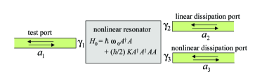
Figure 1: The model includes nonlinear resonator coupled to three ports, a test port, a linear dissipation port and a non-linear one.

It is convenient to write the Hamiltonian as a sum of terms,

$$H=H_{r}+H_{a_{1}}+H_{a_{2}}+H_{a_{3}}+H_{T_{1}}+H_{T_{2}}+H_{T_{3}}\ ,$$ (4)

each representing the Hamiltonian for a component of the system.

The three ports coupled to the resonator (see Fig. 1) serve as baths. One bath models the external modes that couple to the resonator mode through the port that serves both as the input port and as the output port. The Hamiltonian $H_{a1}$ for this bath is given by

$$H_{a1}=\int d\omega\hbar\omega a_{1}^{\dagger}(\omega)a_{1}(\omega)\ .$$ (5)

The other two baths are associated with the linear and nonlinear cavity losses and their Hamiltonians are given by

$$H_{a2}=\int d\omega\hbar\omega a_{2}^{\dagger}(\omega)a_{2}(\omega)$$ (6)

and

$$H_{a3}=\int d\omega\hbar\omega a_{3}^{\dagger}(\omega)a_{3}(\omega)\ .$$ (7)

The linear coupling of the bath modes $a_{1}$ and $a_{2}$ to the cavity mode $A$ is modeled by the hopping Hamiltonians

$$H_{T_{1}}=\hbar\int d\omega[\kappa_{1}A^{\dagger}a_{1}(\omega)+\kappa_{1}^{\ast}a_{1}^{\dagger}(\omega)A]$$ (8)

and

$$H_{T_{2}}=\hbar\int d\omega[\kappa_{2}A^{\dagger}a_{2}(\omega)+\kappa_{2}^{\ast}a_{2}^{\dagger}(\omega)A]\ .$$ (9)

The two-photon absorptive coupling of the resonator mode to the bath modes $a_{3}$ is modeled by a hopping Hamiltonian in which two cavity photons are destroyed for every bath photon created tornau74 ; agarwal86 ; gilles93 ; ezaki99 ; kitamura99

$$H_{T_{3}}=\hbar\int d\omega[\kappa_{3}A^{\dagger}A^{\dagger}a_{3}(\omega)+\kappa_{3}^{\ast}a_{3}^{\dagger}(\omega)AA]\ .$$ (10)

All the modes in this model satisfy the usual boson commutation relations.

III The equations of motion

Since the creation and annihilation operators appearing in Eqs. (LABEL:eq:h2) through (10) do not have an explicit time dependence, the Heisenberg equation of motion for these operators has the form

$$i\hbar\frac{dO}{dt}=[O,H]$$ (11)

where $H$ is the total Hamiltonian. Using the boson commutation relation for the cavity mode

$$[A,A^{\dagger}]=AA^{\dagger}-A^{\dagger}A=1\ ,$$ (12)

one has

$$\frac{dA}{dt} =-i\omega_{0}A-iKA^{\dagger}AA$$ (13)

$$-i\kappa_{1}\int d\omega a_{1}(\omega)-i\kappa_{2}\int d\omega a_{2}(\omega)-i2\kappa_{3}\int d\omega A^{\dagger}a_{3}(\omega)\ .$$

Using the boson commutation relations for the bath modes

$$[a_{i}(\omega),a_{j}^{\dagger}(\omega^{\prime})] =\delta_{i,j}\delta(\omega-\omega^{\prime})$$ (14)

$$\ [a_{i}(\omega),a_{j}(\omega^{\prime})] =0\ ,$$ (15)

one obtains the following equations for the bath modes $a_{1}(\omega)$, $a_{2}(\omega)$, and $a_{3}(\omega)$:

$$\frac{da_{1}(\omega)}{dt}=-i\omega a_{1}(\omega)-i\kappa_{1}^{\ast}A\ ,$$ (16)

$$\frac{da_{2}(\omega)}{dt}=-i\omega a_{2}(\omega)-i\kappa_{2}^{\ast}A\ ,$$ (17)

and

$$\frac{da_{3}(\omega)}{dt}=-i\omega a_{3}(\omega)-i\kappa_{3}^{\ast}AA\ .$$ (18)

Using the standard methods of Gardiner and Collett gardiner85 , these equations yield the following equation for the cavity mode $A$ driven by the incoming bath modes $a_{i}^{in}$:

$$\frac{dA}{dt} =-i\omega_{0}A-iKA^{\dagger}AA-\gamma A-\gamma_{3}A^{\dagger}AA$$ (19)

$$\ \ \ -\ i\sqrt{2\gamma_{1}}e^{i\phi_{1}}a_{1}^{in}(t)-i\sqrt{2\gamma_{2}}e^{i\phi_{2}}a_{2}^{in}(t)$$

$$-i2\sqrt{\gamma_{3}}e^{i\phi_{3}}A^{\dagger}a_{3}^{in}(t)\ .$$

where

$$\gamma=\gamma_{1}+\gamma_{2}$$ (20)

and the $\kappa_{i}$, which in general can be complex, have been reexpressed in terms of the positive real constants $\gamma_{i}$ and the phases $\phi_{i}$ according to

$$\kappa_{1} =\sqrt{\frac{\gamma_{1}}{\pi}}e^{i\phi_{1}}\ ,$$ (21)

$$\kappa_{2} =\sqrt{\frac{\gamma_{2}}{\pi}}e^{i\phi_{2}}\ ,$$ (22)

$$\kappa_{3} =\sqrt{\frac{\gamma_{3}}{2\pi}}e^{i\phi_{3}}\ .$$ (23)

Expressions for $\gamma_{2}$ and $\gamma_{3}$ in terms of linear and nonlinear resistance of the stripline (see Eq. (2)) are given in Eqs. (165), (166). In addition, the methods of Gardiner and Collett gardiner85 yield the following relations between the outgoing bath modes $a_{i}^{out}$, the incoming bath modes $a_{i}^{in}$, and the cavity mode $A$

$$a_{1}^{out}(t)-a_{1}^{in}(t)=-i\sqrt{2\gamma_{1}}e^{-i\phi_{1}}A(t)\ ,$$ (24)

$$a_{2}^{out}(t)-a_{2}^{in}(t)=-i\sqrt{2\gamma_{2}}e^{-i\phi_{2}}A(t)\ ,$$ (25)

$$a_{3}^{out}(t)-a_{3}^{in}(t)=-i\sqrt{\gamma_{3}}e^{-i\phi_{3}}A(t)A(t)\ .$$ (26)

In obtaining these equations a Markov approximation gardiner85 has been made such that the boson annihilation operators $a_{i}^{in}(t)$ satisfy the commutation relations

$$[a_{i}^{in}(t),a_{j}^{in\dagger}(t^{\prime})]=\delta_{i,j}\delta(t-t^{\prime})\ ,$$ (27)

$$[a_{i}^{in}(t),a_{j}^{in}(t^{\prime})]=0\ .$$ (28)

IV Response to a classical pump

Operated as a negative-resistance reflection amplifier, an intense sinusoidal field, called the pump, is delivered to the input port of the device. Signals having frequencies to either side of the pump, but lying within the bandwidth of the device, will be amplified. The linearization procedure is now carried out in which the signals entering the input port and the noise entering the loss ports are considered to be small compared to the pump. The first step is to calculate the classical response of the device to an intense pump in the absence of signal and noise. The solution is then used to calculate the linearized response of the device in the presence of signal and noise.

In order to obtain the response of the device to a classical pump in the absence of signal and noise one sets the incoming noise terms to zero

$$a_{2}^{in} =0\ ,$$ (29)

$$a_{3}^{in} =0\ .$$ (30)

The incoming pump is written as

$$a_{1}^{in}=b_{1}^{in}e^{-i(\omega_{p}t+\psi_{1})}$$ (31)

where $b_{1}^{in}$ is a real constant, $\omega_{p}$ is the pump frequency, and $\psi_{1}$ is the pump phase. The outgoing field will also have an oscillatory time dependence of frequency $\omega_{p}$ and can be written as

$$a_{1}^{out}=b_{1}^{out}e^{-i(\omega_{p}t+\psi_{1})}$$ (32)

where $b_{1}^{out}$ may be a complex constant. Writing $A$ as

$$A=Be^{-i(\omega_{p}t+\phi_{B})}$$ (33)

where $B$ is a positive real constant, the equations of motion, Eqs. (19) and (24), yield

$$[i(\omega_{0}-\omega_{p})+\gamma]B+(iK+\gamma_{3})B^{3}=-i\sqrt{2\gamma_{1}}b_{1}^{in}e^{i(\phi_{1}+\phi_{B}-\psi_{1})}$$ (34)

and

$$b_{1}^{out}=b_{1}^{in}-i\sqrt{2\gamma_{1}}Be^{-i(\phi_{1}+\phi_{B}-\psi_{1})}\ .$$ (35)

Multiplying each side of the Eq. (34) by its complex conjugate and introducing

$$E=B^{2}\ ,$$ (36)

one obtains

$$E^{3}+\frac{2[(\omega_{0}-\omega_{p})K+\gamma\gamma_{3}]}{K^{2}+\gamma_{3}^{2}}E^{2}+\frac{(\omega_{0}-\omega_{p})^{2}+\gamma^{2}}{K^{2}+\gamma_{3}^{2}}E$$

$$-\frac{2\gamma_{1}}{K^{2}+\gamma_{3}^{2}}(b_{1}^{in})^{2}=0\ .$$ (37)

This cubic equation will have one real solution and two complex solutions or three real solutions. For the case when two of the solutions are complex, the real solution is the physical solution. If there are three solutions, two will be stable and one unstable, and the device will exhibit bistability. Once $E$ and, hence, $B$ have been determined from Eqs. (37) and (36), the phase $\phi_{B}$ can be determined from Eq. (34) and the amplitude of the reflected pump can then be computed from Eq. (35). In Fig. 2 (a), (d), and (g) plots of $B$ as a function of frequency for three different incoming pump amplitudes are shown. The frequency pulling of the cavity resonance is clearly seen in (d) and (g) as the incoming pump amplitude $b_{1}^{in}$ is increased. Also plotted in Fig. 2 (b), (e), and (h) is the reflection coefficient $|b_{1}^{out}/b_{1}^{in}|$ for the reflected pump amplitude as a function of frequency. If no power were absorbed by the cavity, the reflection coefficient would be unity. One sees a dip in the reflected power at the cavity resonance. As the incoming pump amplitude is increased, this absorption feature also shows frequency pulling, as can be seen in (e) and (h).

Figure 2: The cavity-mode amplitude $\left|B\right|$, the reflection amplitude $\left|b_{1}^{out}/b_{1}^{in}\right|$, and the intermodulation gain $G_{I}$ for vanishing offset frequency $\omega=0$ shown for sub-critical case $b_{1}^{in}=0.5b_{1C}^{in}$, critical case $b_{1}^{in}=b_{1C}^{in}$, and above-critical case $b_{1}^{in}=2b_{1C}^{in}$. In all cases $K=-10^{-4}\omega_{0}$, $\gamma_{1}=0.01\omega_{0},$ $\gamma_{2}=1.1\gamma_{1}$, and $\gamma_{3}=0.01K/\sqrt{3}$. For $b_{1}^{in}>b_{1C}^{in}$ the response becomes multi-value function of frequency in some frequency range.

IV.1 Special operating points

As a function of the pump frequency $\omega_{p}$, $B$ will have the form of the distorted Lorentzian curve (see Fig. 2 (a), (d), and (g)) exhibited by Duffing oscillators nayfeh ; landau ; yurke95 . The maximum of the response curve occurs when $\partial E/\partial\omega_{p}=0$. This condition yields

$$\omega_{0}-\omega_{p}+KE=0\ ,$$ (38)

that is, the peak of the resonance curve is shifted by an amount $KB^{2}$. The points of instability where the system will switch from one of the two bistable states to the other are located where $\partial\omega_{p}/\partial E=0$. This condition is satisfied when

$$(\gamma+2\gamma_{3}E)^{2}=(K^{2}+\gamma_{3}^{2})E^{2}-(\omega_{0}-\omega_{p}+2KE)^{2}\ .$$ (39)

When, in addition, $\partial^{2}\omega_{p}/\partial E^{2}=0$, the two points of instability coalesce into a single point. The condition $\partial^{2}\omega_{p}/\partial E^{2}=0$ is satisfied when

$$6(K^{2}+\gamma_{3}^{2})E+4[(\omega_{0}-\omega_{p})K+\gamma\gamma_{3}]=0\ .$$ (40)

Large parametric gain is achieved at points where the slope of $E$ with respect to $\omega_{p}$ becomes infinite, but in order to remain stable it is desirable to operate the reflection parametric amplifier near the critical point with parameters chosen so that the Duffing curve does not have a bistable region. It is a straightforward exercise to show that in order for the resonance curve to have a critical point at which both Eqs. (39) and (40) are satisfied, one must have

$$|K|>\sqrt{3}\gamma_{3}\ .$$ (41)

At the critical point one has

$$E_{c}=\frac{2\gamma}{\sqrt{3}(|K|-\sqrt{3}\gamma_{3})}$$ (42)

and

$$\omega_{0}-\omega_{p}=-\gamma\frac{K}{|K|}\left[\frac{4\gamma_{3}|K|+\sqrt{3}(K^{2}+\gamma_{3}^{2})}{K^{2}-3\gamma_{3}^{2}}\right]\ .$$ (43)

The incoming pump amplitude required for operation at the critical point is given by

$$(b_{1c}^{in})^{2}=\frac{4}{3\sqrt{3}}\frac{\gamma^{3}(K^{2}+\gamma_{3}^{2})}{\gamma_{1}(|K|-\sqrt{3}\gamma_{3})^{3}}\ .$$ (44)

Thus, the input power required for driving the system into the threshold of bistability (critical point) is increased in the presence of two-photon losses. Moreover, when $\gamma_{3}$ exceeds the value of $|K|/\sqrt{3}$ the bistability regime becomes inaccessible (see Eq. (41)).

When $\gamma_{3}=0$ these reduce to

$$E_{c} =\frac{2\sqrt{3}\gamma}{3|K|}\ ,$$ (45)

$$\omega_{0}-\omega_{p} =-\sqrt{3}\gamma\frac{K}{|K|}\ ,$$ (46)

$$(b_{1c}^{in})^{2} =\frac{4}{3\sqrt{3}}\frac{\gamma^{3}}{\gamma_{1}|K|}\ .$$ (47)

In panel (d) of Fig. 2 the amplitude of the cavity mode as a function of frequency has been plotted for the case when the incoming pump amplitude is that of the critical pump amplitude. One sees that the line shape of the cavity mode is vertical at a point on the lower side of the resonance. The line shape of the reflected power is shown in panel (e) of Fig. 2.

V Linearization

A linearized analysis is now performed in which the incoming signal and the noise from the losses are regarded as small compared to the pump. To that end we write

$$a_{1}^{in}=b_{1}^{in}e^{-i(\omega_{p}t+\psi_{1})}+c_{1}^{in}e^{-i\omega_{p}t}\ ,$$ (48)

$$a_{2}^{in}=c_{2}^{in}e^{-i\omega_{p}t}\ ,$$ (49)

$$a_{3}^{in}=c_{3}^{in}e^{-i\omega_{p}t}\ ,$$ (50)

$$a_{1}^{out}=b_{1}^{out}e^{-i(\omega_{p}t+\psi_{1})}+c_{1}^{out}e^{-i\omega_{p}t}\ ,$$ (51)

$$a_{2}^{out}=b_{2}^{out}e^{-i\omega_{p}t}+c_{2}^{out}e^{-i\omega_{p}t}\ ,$$ (52)

$$a_{3}^{out}=b_{3}^{out}e^{-i\omega_{p}t}+c_{3}^{out}e^{-i\omega_{p}t}\ ,$$ (53)

and

$$A=Be^{-i(\omega_{p}t+\phi_{B})}+ae^{-i\omega_{p}t}$$ (54)

where $B$, $b_{1}^{out}$, $b_{2}^{out}$ and $b_{3}^{out}$ constitute the solution for the response of the system to a classical pump in the absence of signal and noise. The properties of this solution have already been discussed in Section 4. The $c_{1}^{in}$, $c_{2}^{in}$, $c_{3}^{in}$, $c_{1}^{out}$, $c_{2}^{out}$, $c_{3}^{out}$, and $a$ are regarded as small and will be kept only up to linear order. Substituting these into the equations of motion yields

$$\frac{da}{dt} =-[i(\omega_{0}-\omega_{p})+\gamma]a-2(iK+\gamma_{3})B^{2}a$$

$$-(iK+\gamma_{3})B^{2}e^{-i2\phi_{B}}a^{\dagger}-\ i\sqrt{2\gamma_{1}}e^{i\phi_{1}}c_{1}^{in}$$

$$-i\sqrt{2\gamma_{2}}e^{i\phi_{2}}c_{2}^{in}-i2\sqrt{\gamma_{3}}Be^{i(\omega_{p}t+\phi_{B}+\phi_{3})}c_{3}^{in}\ ,$$ (55)

$$c_{1}^{out}-c_{1}^{in}=-i\sqrt{2\gamma_{1}}e^{-i\phi_{1}}a\ ,$$ (56)

$$c_{2}^{out}-c_{2}^{in}=-i\sqrt{2\gamma_{2}}e^{-i\phi_{2}}a\ ,$$ (57)

$$c_{3}^{out}-c_{3}^{in}=-i2\sqrt{\gamma_{3}}Be^{-i(\omega_{p}t+\phi_{B}+\phi_{3})}a\ .$$ (58)

VI Solving the linearized equation

Introducing

$$W=i(\omega_{0}-\omega_{p})+\gamma+2(iK+\gamma_{3})B^{2}\ ,$$ (59)

$$V=(iK+\gamma_{3})B^{2}e^{-2i\phi_{B}}\ ,$$ (60)

and

$$F =-i\sqrt{2\gamma_{1}}e^{i\phi_{1}}c_{1}^{in}-i\sqrt{2\gamma_{2}}e^{i\phi_{2}}c_{2}^{in}$$

$$\ \ \ -\ i2\sqrt{\gamma_{3}}Be^{i(\omega_{p}t+\phi_{B}+\phi_{3})}c_{3}^{in}\ ,$$ (61)

the linearized equation of motion can be written in the form

$$\frac{da}{dt}+Wa+Va^{\dagger}=F\ .$$ (62)

From this last equation one obtains

$$\frac{d^{2}a}{dt^{2}}+2\Re(W)\frac{da}{dt}+(|W|^{2}-|V|^{2})a=\Gamma(t)$$ (63)

where

$$\Gamma(t)=\frac{dF}{dt}+W^{\ast}F-VF^{\dagger}(t)\ .$$ (64)

Writing

$$a=e^{-\lambda t}\ ,$$ (65)

the characteristic equation for the homogenous equation is given by

$$\lambda^{2}-2\Re(\omega)\lambda+|W|^{2}-|V|^{2}=0\ .$$ (66)

This has the two roots

$$\lambda_{0}=\Re(W)-\sqrt{\Re^{2}(W)-|W|^{2}+|V|^{2})}\ ,$$ (67)

$$\lambda_{1}=\Re(W)+\sqrt{\Re^{2}(W)-|W|^{2}+|V|^{2})}\ ,$$ (68)

or

$$\lambda_{0}=\gamma+2\gamma_{3}B^{2}-\sqrt{(K^{2}+\gamma_{3}^{2})B^{4}-(\omega_{0}-\omega_{p}+2KB^{2})^{2}}\ ,$$ (69)

$$\lambda_{1}=\gamma+2\gamma_{3}B^{2}+\sqrt{(K^{2}+\gamma_{3}^{2})B^{4}-(\omega_{0}-\omega_{p}+2KB^{2})^{2}}\ .$$ (70)

The root $\lambda_{0}$ is zero when Eq. (39) is satisfied, that is, one has critical slowing down at the points where the slope of $E$ with respect to $\omega_{p}$ is infinite.

Introducing the Fourier transforms

$$a(t)=\frac{1}{\sqrt{2\pi}}\int_{-\infty}^{\infty}d\omega a(\omega)e^{-i\omega t}\ ,$$ (71)

$$c_{1}(t)=\frac{1}{\sqrt{2\pi}}\int_{-\infty}^{\infty}d\omega c_{1}(\omega)e^{-i\omega t}\ ,$$ (72)

$$c_{2}(t)=\frac{1}{\sqrt{2\pi}}\int_{-\infty}^{\infty}d\omega c_{2}(\omega)e^{-i\omega t}\ ,$$ (73)

$$c_{3}(t)=\frac{1}{\sqrt{2\pi}}\int_{-\infty}^{\infty}d\omega c_{3}(\omega)e^{-i\omega t}\ ,$$ (74)

$$\Gamma(t)=\frac{1}{\sqrt{2\pi}}\int_{-\infty}^{\infty}d\omega\Gamma(\omega)e^{-i\omega t}\ ,$$ (75)

Eq. (63) yields

$$a(\omega)=\frac{\Gamma(\omega)}{-\omega^{2}-2i\omega\Re(W)+(|W|^{2}-|V|^{2})}\ .$$ (76)

In terms of the roots of the characteristic equation this can be written as

$$a(\omega)=\frac{\Gamma(\omega)}{(-i\omega+\lambda_{0})(-i\omega+\lambda_{1})}$$ (77)

where

$$\Gamma(\omega) =-i\sqrt{2\gamma_{1}}[(-i\omega+W^{\ast})e^{i\phi_{1}}c_{1}^{in}(\omega)-Ve^{-i\phi_{1}}c_{1}^{in\dagger}(-\omega)]$$

$$-\ i\sqrt{2\gamma_{2}}[(-i\omega+W^{\ast})e^{i\phi_{2}}c_{2}^{in}(\omega)-Ve^{-i\phi_{2}}c_{2}^{in\dagger}(-\omega)]$$

$$-\ i2\sqrt{\gamma_{3}}B[(-i\omega+W^{\ast})e^{i(\phi_{B}+\phi_{3})}c_{3}^{in}(\omega_{p}+\omega)$$

$$\ -\ Ve^{-i(\phi_{B}+\phi_{3})}c_{3}^{in\dagger}(\omega_{p}-\omega)]\ .$$ (78)

VI.1 The output field

From Eq. (24) one obtains

$$c_{1}^{out}(\omega)=c_{1}^{in}(\omega)-i\sqrt{2\gamma_{1}}e^{-i\phi_{1}}a(\omega)\ .$$ (79)

Substituting Eq. (77) into this equation yields

$$c_{1}^{out}(\omega)$$

$$=\frac{(-i\omega+\lambda_{0})(-i\omega+\lambda_{1})c_{1}^{in}(\omega)-i\sqrt{2\gamma_{1}}e^{-i\phi_{1}}\Gamma(\omega)}{(-i\omega+\lambda_{0})(-i\omega+\lambda_{1})}$$ (80)

or

$$c_{1}^{out}(\omega)$$

$$=\frac{(-i\omega+\lambda_{0})(-i\omega+\lambda_{1})-2\gamma_{1}(-i\omega+W^{\ast})}{(-i\omega+\lambda_{0})(-i\omega+\lambda_{1})}c_{1}^{in}(\omega)$$

$$+\ \frac{2\gamma_{1}Ve^{-i2\phi_{1}}}{(-i\omega+\lambda_{0})(-i\omega+\lambda_{1})}c_{1}^{in\dagger}(-\omega)$$

$$-\ \frac{2\sqrt{\gamma_{1}\gamma_{2}}(-i\omega+W^{\ast})e^{-i(\phi_{1}-\phi_{2})}}{(-i\omega+\lambda_{0})(-i\omega+\lambda_{1})}c_{2}^{in}(\omega)$$

$$+\ \frac{2\sqrt{\gamma_{1}\gamma_{2}}Ve^{-i(\phi_{1}+\phi_{2})}}{(-i\omega+\lambda_{0})(-i\omega+\lambda_{1})}c_{2}^{in\dagger}(-\omega)$$

$$-\ \frac{2\sqrt{2\gamma_{1}\gamma_{3}}B(-i\omega+W^{\ast})e^{-i(\phi_{1}-\phi_{B}-\phi_{3})}}{(-i\omega+\lambda_{0})(-i\omega+\lambda_{1})}c_{3}^{in}(\omega_{p}+\omega)$$

$$+\frac{2\sqrt{2\gamma_{1}\gamma_{3}}BVe^{-i(\phi_{1}+\phi_{3}+\phi_{B})}}{(-i\omega+\lambda_{0})(-i\omega+\lambda_{1})}c_{3}^{in\dagger}(\omega_{p}-\omega)\ .$$ (81)

The linearized solution to the equations of motion has now been obtained. We will now evaluate the properties of this solution for various kinds of inputs.

VII Parametric and intermodulation gain

The parametric gain and the intermodulation gain are calculated by taking $c_{1}^{in}(\omega)$ to represent a classical signal at frequency $\omega_{p}+\omega$. Setting all other signal and noise inputs to zero, Eq. (81) yields the following power gain for the reflected signal:

$$G_{S} \equiv\frac{|c_{1}^{out}(\omega)|^{2}}{|c_{1}^{in}(\omega)|^{2}}$$

$$=\frac{|(-i\omega+\lambda_{0})(-i\omega+\lambda_{1})-2\gamma_{1}(-i\omega+W^{\ast})|^{2}}{(\omega^{2}+\lambda_{0}^{2})(\omega^{2}+\lambda_{1}^{2})}\ .$$ (82)

When this quantity becomes greater than unity one has parametric amplification of the signal.

As seen from Eq. (81), a signal $c_{in}(-\omega)$ injected at frequency $\omega_{p}-\omega$ will generate an output signal at frequency $\omega_{p}+\omega$. This frequency conversion is quantified by the intermodulation conversion gain defined by

$$G_{I} \equiv\frac{|c_{1}^{out}(\omega)|^{2}}{|c_{1}^{in}(-\omega)|^{2}}$$

$$=\frac{4\gamma_{1}^{2}|V|^{2}}{(\omega^{2}+\lambda_{0}^{2})(\omega^{2}+\lambda_{1}^{2})}\ .$$ (83)

Since the output signal at $\omega_{p}+\omega$ is separated in frequency from the input signal, the measurement of the intermodulation gain is a particularly sensitive method for measuring the strength of the nonlinearities. We note that, even without power gain, devices capable of producing intermodulation signals are useful as mixers. When $\omega=0$, both the expression for $G_{S}$ and the expression for $G_{I}$ will have $\lambda_{0}^{2}\lambda_{1}^{2}$ in the denominator. As one approaches an operating point where the slope of $E$ with respect to $\omega_{p}$ becomes infinite, both the parametric gain and the intermodulation conversion gain will diverge. Hence, it is near the instability points where the device can exhibit large gains. Panels (c), (f), and (i) of Fig. 2 show the behavior of the intermodulation gain as the pump amplitude is increased from half critical (c) to critical (f) to twice critical (i) as a function of frequency. As depicted in panel (f) at the critical point the intermodulation gain diverges. Above critical, as shown in panel (i), the intermodulation gain diverges as one approaches the points of infinite slope on the resonance curve (g).

VIII Noise squeezing

Because of intermodulation gain, a parametric amplifier can establish correlations yurke85 between the output at $\omega_{p}+\omega$ and $\omega_{p}-\omega$. When delivered to a mixer whose local oscillator is phase-locked to the pump these correlations can result in noise fluctuations reduced below that which the mixer would see if the signal delivered to the parametric amplifier were, instead, directly delivered to the mixer. This noise reduction is called squeezing, and it can occur with either thermal or quantum noise movshovich90 . We now obtain expressions that will allow one to calculate the degree of thermal or quantum noise squeezing. For such a calculation the $c_{1}^{in}$, $c_{2}^{in}$, $c_{3}^{in}$, $c_{1}^{out}$, $c_{2}^{out}$, $c_{3}^{out}$ are again treated as quantum mechanical operators satisfying commutation relations of the form Eqs. (27) and (28).

The output of a mixer, operated in the homodyne mode in which the local oscillator frequency $\omega_{LO}$ and the pump frequency $\omega_{p}$ are equal and in which the input at the signal frequency $\omega_{LO}+\omega$ and at the image frequency $\omega_{LO}-\omega$ are both regarded as signal, is given by yurke89

$$I_{D}(\omega)=c_{1}^{out\dagger}(-\omega)e^{-i\phi_{LO}}+c_{1}^{out}(\omega)e^{i\phi_{LO}}$$ (84)

where $\phi_{LO}$ is the local oscillator phase. To evaluate the mean value and the power spectrum for the homodyne detector output it is necessary to specify the density matrix for the signal and noise entering the parametric amplifier. Here we consider the case when these inputs consist of Nyquist noise. In this case one has

$$\langle c_{i}^{in}(\omega)\rangle=0\ ,$$ (85)

$$\langle c_{i}^{in\dagger}(\omega)c_{j}^{in}(\omega^{\prime})\rangle=\frac{e^{-\beta_{i}\hbar\omega_{p}}}{1-e^{-\beta_{i}\hbar\omega_{p}}}\delta_{i,j}\delta(\omega-\omega^{\prime})\ ,$$ (86)

and

$$\langle c_{i}^{in}(\omega)c_{j}^{in}(\omega^{\prime})\rangle=0\ .$$ (87)

Here

$$\beta_{i}=\frac{1}{k_{B}T_{i}}\ ,$$ (88)

where $k_{B}$ is Boltzmann’s constant and $T_{i}$ is the absolute temperature of the bath for which $c_{i}^{in}(\omega)$ is the incoming mode. We thus allow each of the baths to be at a different temperature. In writing Eq. (86) we have made the approximation that the frequencies $\omega$ of interest are small compared to $\omega_{p}$.

Because Eq. (81) is linear in the $c_{i}^{in}(\omega)$ it is evident that

$$\langle I_{D}(\omega)\rangle=0\ ,$$ (89)

that is, the homodyne detector output consists of noise fluctuations with zero mean. Because of the boson commutation relations, one has

$$\langle I_{D}^{\dagger}(\omega)I_{D}(\omega^{\prime})\rangle=P(\omega)\delta(\omega-\omega^{\prime})$$ (90)

where $P(\omega)$ is the noise power spectrum of the homodyne detector output. Equation (81) can be rewritten as

$$c_{1}^{out}(\omega) =A_{1}(\omega)c_{1}^{in}(\omega)+B_{1}(\omega)c_{1}^{in\dagger}(-\omega)$$

$$+\ A_{2}(\omega)c_{2}^{in}(\omega)+B_{2}(\omega)c_{2}^{in\dagger}(-\omega)$$

$$+\ A_{3}(\omega)c_{3}^{in}(\omega_{p}+\omega)+B_{3}(\omega)c_{3}^{in\dagger}(\omega_{p}-\omega)$$ (91)

where

$$A_{1}(\omega)=\frac{(-i\omega+\lambda_{0})(-i\omega+\lambda_{1})-2\gamma_{1}(-i\omega+W^{\ast})}{(-i\omega+\lambda_{0})(-i\omega+\lambda_{1})}\ ,$$ (92)

$$B_{1}(\omega)=\frac{2\gamma_{1}Ve^{-i2\phi_{1}}}{(-i\omega+\lambda_{0})(-i\omega+\lambda_{1})}\ ,$$ (93)

$$A_{2}(\omega)=-\frac{2\sqrt{\gamma_{1}\gamma_{2}}(-i\omega+W^{\ast})e^{-i(\phi_{1}-\phi_{2})}}{(-i\omega+\lambda_{0})(-i\omega+\lambda_{1})}\ ,$$ (94)

$$B_{2}(\omega)=\frac{2\sqrt{\gamma_{1}\gamma_{2}}Ve^{-i(\phi_{1}+\phi_{2})}}{(-i\omega+\lambda_{0})(-i\omega+\lambda_{1})}\ ,$$ (95)

$$A_{3}(\omega)=-\ \frac{2\sqrt{2\gamma_{1}\gamma_{3}}B(-i\omega+W^{\ast})e^{-i(\phi_{1}-\phi_{B}-\phi_{3})}}{(-i\omega+\lambda_{0})(-i\omega+\lambda_{1})}\ ,$$ (96)

$$B_{3}(\omega)=\frac{2\sqrt{2\gamma_{1}\gamma_{3}}BVe^{-i(\phi_{1}+\phi_{3}+\phi_{B})}}{(-i\omega+\lambda_{0})(-i\omega+\lambda_{1})}\ .$$ (97)

Substituting Eq. (91) into Eq. (84), evaluating $\langle I_{D}^{\dagger}(\omega)I_{D}(\omega^{\prime})\rangle$ using Eq. (86), and then reading off the power spectrum using Eq. (90), one obtains

$$P(\omega) =|e^{-i\phi_{LO}}A_{1}^{\ast}(\omega)+e^{i\phi_{LO}}B_{1}(-\omega)|^{2}\frac{e^{-\beta_{1}\hbar\omega_{p}}}{1-e^{-\beta_{1}\hbar\omega_{p}}}$$

$$+\ |e^{i\phi_{LO}}A_{1}(-\omega)+e^{-i\phi_{LO}}B_{1}^{\ast}(\omega)|^{2}\frac{1}{1-e^{-\beta_{1}\hbar\omega_{p}}}$$

$$+\ |e^{-i\phi_{LO}}A_{2}^{\ast}(\omega)+e^{i\phi_{LO}}B_{2}(-\omega)|^{2}\frac{e^{-\beta_{2}\hbar\omega_{p}}}{1-e^{-\beta_{2}\hbar\omega_{p}}}$$

$$+\ |e^{i\phi_{LO}}A_{2}(-\omega)+e^{-i\phi_{LO}}B_{2}^{\ast}(\omega)|^{2}\frac{1}{1-e^{-\beta_{2}\hbar\omega_{p}}}$$

$$+\ |e^{-i\phi_{LO}}A_{3}^{\ast}(\omega)+e^{i\phi_{LO}}B_{3}(-\omega)|^{2}\frac{e^{-\beta_{3}\hbar\omega_{p}}}{1-e^{-\beta_{3}\hbar\omega_{p}}}$$

$$+\ |e^{i\phi_{LO}}A_{3}(-\omega)+e^{-i\phi_{LO}}B_{3}^{\ast}(\omega)|^{2}\frac{1}{1-e^{-\beta_{3}\hbar\omega_{p}}}\ .$$ (98)

This formula may be used to compute the noise-power spectrum for any local oscillator phase $\phi_{LO}$ and any set of device parameters. It is useful to consider the case when there is no incoming pump field and the input field and loss baths are all at zero temperature. In this case the field reflected off the input port of the amplifier will consist of vacuum fluctuations, that is,

$$c_{1}^{out}(\omega)|0\rangle=0\ ,$$ (99)

and one obtains

$$\langle I_{D}^{\dagger}(\omega)I_{D}(\omega^{\prime})\rangle=\delta(\omega-\omega^{\prime})$$ (100)

or

$$P(\omega)=1\ .$$ (101)

This sets the vacuum noise level for the conventions we are using. As is shown in Fig. 3 and as will be illustrated with specific examples in the next section, under suitable circumstances it is possible to obtain reflected signals whose noise-power spectrum $P(\omega)$, for certain local oscillator phase settings, is less than 1. Such signals are said to be squeezed below the vacuum noise level. Figure 3 shows the minimum value of $P(\omega)$ as a function of the amplitude of the incoming pump $b_{1}^{in}$ when the bath temperatures are all zero, the strength of the Kerr nonlinearity is chosen to be $K=5\omega_{0}$, and the coupling strength of the signal to the cavity mode is taken to be $\gamma_{1}=0.0001\omega_{0}$. The pump frequency has been chosen to be that of the critical pump frequency. The solid line is the lossless case when $\gamma_{2}=\gamma_{3}=0$. In this case complete squeezing $P(0)=0$ is possible when the incoming pump power is at the critical value, that is, $|b_{1}^{in}/b_{1c}^{in}|=1$. The dashed curve represents the case when the linear dissipation is given by $\gamma_{2}=5\gamma_{1}$ and the nonlinear dissipation $\gamma_{3}$ is zero. In general, the presence of linear dissipation reduces the amount of achievable squeezing. The dotted line depicts the case when the linear dissipation is zero and the nonlinear dissipation is given by $\gamma_{3}=0.5K/\sqrt{3}$. Nonlinear dissipation also tends to reduce the amount of squeezing that can be produced. However, nonlinear dissipation can produce some squeezing in the absence of a Kerr medium, as we discuss below.

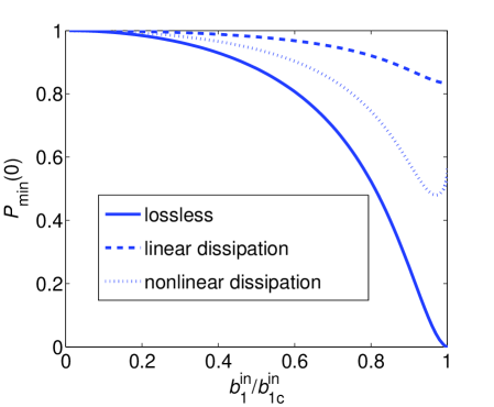
Figure 3: Examples of achievable degree of squeezing, $P_{min}(0)$ vs. $b_{1}^{in}/b_{1c}^{in}$. In all plots $T_{1}=T_{2}=T_{3}=0$, $K=5\omega_{0}$, $\gamma_{1}=0.0001\omega_{0}$, and the pump frequency $\omega_{p}$ obtains its critical value, as given by Eq. 43. The solid line represents the lossless case, where $\gamma_{2}=\gamma_{3}=0$.  The dashed line represents the case of linear dissipation where $\gamma_{2}=5\gamma_{1}$ and $\gamma_{3}=0$, while the dotted line represents the case of nonlinear dissipation where $\gamma_{2}=0$ and $\gamma_{3}=0.5K/\sqrt{3}$.

VIII.1 Special cases

It is instructive to evaluate Eq. (98) for a few specific cases. In particular, the power spectrum at $\omega=0$ reduces to

$$P(0) =|e^{-i\phi_{LO}}A_{1}^{\ast}(0)+e^{i\phi_{LO}}B_{1}(0)|^{2}\coth\left(\frac{\hbar\omega_{p}}{2k_{B}T_{1}}\right)$$

$$+\ |e^{-i\phi_{LO}}A_{2}^{\ast}(0)+e^{i\phi_{LO}}B_{2}(0)|^{2}\coth\left(\frac{\hbar\omega_{p}}{2k_{B}T_{2}}\right)$$

$$+\ |e^{-i\phi_{LO}}A_{3}^{\ast}(0)+e^{i\phi_{LO}}B_{3}(0)|^{2}\coth\left(\frac{\hbar\omega_{p}}{2k_{B}T_{3}}\right)\ .$$ (102)

Further simplification results from considering the case when the internal losses are all zero. In this case $\gamma_{2}=0$ and $\gamma_{3}=0$. Thus, the terms in Eq. (VIII.1) corresponding to internally generated noise vanish and one obtains

$$P(0)=|e^{-i\phi_{LO}}A_{1}^{\ast}(0)+e^{i\phi_{LO}}B_{1}(0)|^{2}\coth\left(\frac{\hbar\omega_{p}}{2k_{B}T_{1}}\right)\ .$$ (103)

Writing

$$A_{1}(0) =|A_{1}(0)|e^{i\phi_{A}}\ ,$$ (104)

$$B_{1}(0) =|B_{1}(0)|e^{i\phi_{B}}\ ,$$ (105)

one has

$$P(0)=\left||A_{1}(0)|+|B_{1}(0)|e^{i\psi}\right|^{2}\coth\left(\frac{\hbar\omega_{p}}{2k_{B}T_{1}}\right)$$ (106)

where

$$\psi=2\phi_{LO}-\phi_{A}+\phi_{B}\ .$$ (107)

$P(0)$ is maximized when the local oscillator phase $\phi_{LO}$ is chosen so that

$$e^{i\psi}=1\ .$$ (108)

In this case one obtains

$$P_{max}(0)=(|A_{1}(0)|+|B_{1}(0)|)^{2}\coth\left(\frac{\hbar\omega_{p}}{2k_{B}T_{1}}\right)\ .$$ (109)

$P(0)$ is minimized when the local oscillator phase $\phi_{LO}$ is chosen so that

$$e^{i\psi}=-1\ .$$ (110)

In this case one obtains

$$P_{min}(0)=(|A_{1}(0)|-|B_{1}(0)|)^{2}\coth\left(\frac{\hbar\omega_{p}}{2k_{B}T_{1}}\right)\ .$$ (111)

From Eqs. (107), (108), and (110) it follows that the local oscillator phase at which the spectral density $P(0)$ is minimized differs by $\pi/2$ from the local oscillator phase at which the spectral density is maximized, that is, the signal components minimizing and maximizing the spectral density are in quadrature. It is straightforward to show that

$$|A_{1}(0)|^{2}-|B_{1}(0)|^{2}=1\ .$$ (112)

From this equation and Eqs. (109) and (111), one obtains

$$P_{max}(0)P_{min}(0)=\coth^{2}\left(\frac{\hbar\omega_{p}}{2k_{B}T_{1}}\right)\ .$$ (113)

Hence, in the case of no loss, the degree of amplification and the degree of deamplification of the noise are the same. For this case one also has

$$|B_{1}(0)|=\frac{2\gamma_{1}KB^{2}}{(\omega_{0}-\omega_{p}+2KB^{2})^{2}+\gamma_{1}^{2}-K^{2}B^{4}}\ .$$ (114)

Note that $|B_{1}(0)|$ can be made arbitrarily large by choosing the pump frequency $\omega_{p}$ and the pump amplitude $B$ such that the denominator goes to zero. From this it follows that $P_{max}$ can be made arbitrarily large and $P_{min}$ can be made arbitrarily small. In practice, higher order terms responsible for pump depletion will limit how big $P_{max}$ can be made.

Noise from the losses and gain saturation will limit the maximum degree of noise squeezing to be below that calculated here. This is demonstrated in Figure 3, where the achievable degree of squeezing $P_{min}(0)$ is plotted as a function of $b_{1}^{in}/b_{1c}^{in}$ for some examples in which the linear or nonlinear loss is taken to be nonzero.

The presence of a two-photon loss allows for squeezing even in the absence of a Kerr nonlinearity ezaki99 . Setting $K=0$, $\gamma_{2}=0$, and $\omega_{0}=\omega_{p}$, the greatest degree of squeezing of the output field of the cavity occurs when $\gamma_{1}=3\gamma_{3}B^{2}$. At this operating point $P(0)=2/3$ and the local oscillator phase must be adjusted so that $\cos(2\phi_{LO}-2\phi_{B}-2\phi_{1})=1$.

IX Conclusions

We have presented an analysis of a cavity parametric amplifier employing a Kerr nonlinearity but which also possesses a two-photon loss. We have obtained expressions for the pump amplitude inside the cavity and the reflected pump amplitude for the case when pump saturation can be neglected. We have obtained expressions for the classical gain and the intermodulation gain. These expressions are useful for determining model parameters from experimental data. We have found that in the presence of two photon losses the injected power required for driving the system into the bistable regime is increased. Moreover, this regime becomes inaccessible when $\gamma_{3}$ exceeds the value of $|K|/\sqrt{3}$.

We have also obtained expressions from which one can compute the degree of squeezing that the device exhibits. Both the linear and nonlinear loss tend to degrade the amount of squeezing that can be achieved, although even without a Kerr nonlinearity a modest amount of squeezing can be achieved by the two-photon loss.

Appendix A Nonlinear Kinetic Inductance in Transmission Line Resonator

Consider a lossless linear transmission line with length $l$ extending along the $x$-axis.  Let $q\left(x,t\right)$ be the charge density per unit length and define yurke84

$$Q\left(x,t\right)=\int\limits_{x}^{\infty}dx^{\prime}q\left(x^{\prime},t\right).$$ (115)

Thus $q=-\partial Q/\partial x$, and the voltage across the transmission line is given by

$$V\left(x,t\right)=-\frac{1}{C}\frac{\partial Q}{\partial x},$$ (116)

where $C$ is the capacitance per unit length along the transmission line, whereas the current is given by

$$I\left(x,t\right)=\frac{\partial Q}{\partial t}.$$ (117)

The Lagrangian $\mathcal{L}$ of the system reads

$$\mathcal{L} =\frac{1}{2}\int\limits_{0}^{l}dx\left[LI^{2}-CV^{2}\right]$$ (118)

$$=\frac{1}{2}\int\limits_{0}^{l}dx\left[L\left(\frac{\partial Q}{\partial t}\right)^{2}-\frac{1}{C}\left(\frac{\partial Q}{\partial x}\right)^{2}\right],$$

where $L$ is the inductance per unit length along the transmission line.  The open ends at $x=0$ and $x=l$ impose boundary conditions of vanishing current.

We assume the case of a nonuniform transmission line, where both $C$ and $L$ may depend on $x$. Moreover, the inductance $L$ depends on the current $I$ according to Eq. (1) as a result of nonlinear kinetic inductance.

As a basis for expanding $Q\left(x,t\right)$ as

$$Q\left(x,t\right)=\sum_{n}q_{n}\left(t\right)u_{n}\left(x\right),$$ (119)

we use the solutions of

$$\frac{d}{dx}\left(\frac{1}{C}\frac{du_{n}}{dx}\right)=-\omega_{n}^{2}Lu_{n},$$ (120)

with the boundary conditions of vanishing current

$$u_{n}\left(0\right)=u_{n}\left(l\right)=0.$$ (121)

We assume that the functions $u_{n}\left(x\right)$ are chosen to be real.

For the case of a uniform transmission line resonator, where both $C$ and $L$ are independent on $x$, one has $\omega_{n}=n\pi/l\sqrt{LC}$, where $n$ is an integer. In the nonlinear regime, however, such an equally spaced spectrum may lead to strong inter-mode coupling, where harmonics and sub-harmonics of a driven mode excite other modes. In the present work we assume that such inter-modes effects are avoided by employing a nonuniform resonator.  This allows us to consider only the mode in the resonator which is driven externally.

Using expansion (119)

$$\mathcal{L} =\frac{1}{2}\sum_{n}\sum_{m}\dot{q}_{n}\dot{q}_{m}\int\limits_{0}^{l}dxL_{0}u_{n}u_{m}$$ (122)

$$-\frac{1}{2}\sum_{n}\sum_{m}q_{n}q_{m}\int\limits_{0}^{l}dx\frac{1}{C}\frac{du_{n}}{dx}\frac{du_{m}}{dx}+\Delta\mathcal{L},$$

where

$$\Delta\mathcal{L} =\frac{1}{2I_{c}^{2}}\sum_{n^{\prime},n^{\prime\prime},n^{\prime\prime\prime},n^{\prime\prime\prime\prime}}\dot{q}_{n^{\prime}}\dot{q}_{n^{\prime\prime}}\dot{q}_{n^{\prime\prime\prime}}\dot{q}_{n^{\prime\prime\prime\prime}}$$

$$\times\int\limits_{0}^{l}dx\ u_{n^{\prime}}u_{n^{\prime\prime}}u_{n^{\prime\prime\prime}}u_{n^{\prime\prime\prime\prime}}\Delta L.$$ (123)

We first treat the linear part.  Consider equation (120) for $u_{n}$ multiplied by $u_{m}$ and equation (120) for $u_{m}$ multiplied by $u_{n}$

$$u_{m}\frac{d}{dx}\left(\frac{1}{C}\frac{du_{n}}{dx}\right)=-\omega_{n}^{2}L_{0}u_{n}u_{m},$$ (124)

$$u_{n}\frac{d}{dx}\left(\frac{1}{C}\frac{du_{m}}{dx}\right)=-\omega_{m}^{2}L_{0}u_{n}u_{m}.$$ (125)

Subtracting

$$\frac{d}{dx}\left(u_{m}\frac{1}{C}\frac{du_{n}}{dx}-u_{n}\frac{1}{C}\frac{du_{m}}{dx}\right)=\left(\omega_{m}^{2}-\omega_{n}^{2}\right)L_{0}u_{n}u_{m},$$ (126)

and integrating from $x=0$ to $x=l$ one obtains

$$\left(\omega_{m}^{2}-\omega_{n}^{2}\right)\int\limits_{0}^{l}dxL_{0}u_{n}u_{m}=0.$$ (127)

In general, it can be easily shown that the spectrum of a finite one-dimensional resonator having vanishing current boundary conditions is non-degenerate. Thus, by requiring that the functions $u_{n}\left(x\right)$ are normalized one obtains

$$\int\limits_{0}^{l}dxL_{0}u_{n}u_{m}=\delta_{nm}.$$ (128)

Moreover, integrating by parts and using (120) and the boundary conditions one obtains

$$\int\limits_{0}^{l}dx\frac{1}{C}\frac{du_{n}}{dx}\frac{du_{m}}{dx}=\omega_{n}^{2}\int\limits_{0}^{l}dxL_{0}u_{n}u_{m}=\omega_{n}^{2}\delta_{nm}.$$ (129)

Thus

$$\mathcal{L}=\frac{1}{2}\sum_{n}\left(\dot{q}_{n}^{2}-\omega_{n}^{2}q_{n}^{2}\right)+\Delta\mathcal{L}.$$

The Euler-Lagrange equation is given by

$$\frac{d}{dt}\left(\frac{\partial\mathcal{L}}{\partial\dot{q}_{n}}\right)-\frac{\partial\mathcal{L}}{\partial q_{n}}=0,$$ (130)

thus

$$\ddot{q}_{n}+\omega_{n}^{2}q_{n}+\frac{d}{dt}\left(\frac{\partial\Delta\mathcal{L}}{\partial\dot{q}_{n}}\right)=0.$$ (131)

The variable canonically conjugate to $q_{n}$ is

$$p_{n}=\frac{\partial\mathcal{L}}{\partial\dot{q}_{n}}=\dot{q}_{n}+\frac{\partial\Delta\mathcal{L}}{\partial\dot{q}_{n}}$$ (132)

The Hamiltonian is given by

$$\mathcal{H} =\sum_{n}p_{n}\dot{q}_{n}-\mathcal{L}$$ (133)

$$=\frac{1}{2}\sum_{n}\left[p_{n}^{2}-\left(\frac{\partial\Delta\mathcal{L}}{\partial\dot{q}_{n}}\right)^{2}+\omega_{n}^{2}q_{n}^{2}\right]-\Delta\mathcal{L}.$$

To first order in $\Delta\mathcal{L}$ (or in $\Delta L$)

$$\mathcal{H}=\mathcal{H}_{0}+\mathcal{V},$$ (134)

where

$$\mathcal{H}_{0}=\frac{1}{2}\sum_{n}\left(p_{n}^{2}+\omega_{n}^{2}q_{n}^{2}\right),$$ (135)

and

$$\mathcal{V} =-\frac{1}{2I_{c}^{2}}\sum_{n^{\prime},n^{\prime\prime},n^{\prime\prime\prime},n^{\prime\prime\prime\prime}}p_{n^{\prime}}p_{n^{\prime\prime}}p_{n^{\prime\prime\prime}}p_{n^{\prime\prime\prime\prime}}$$ (136)

$$\times\int\limits_{0}^{l}dx\ u_{n^{\prime}}u_{n^{\prime\prime}}u_{n^{\prime\prime\prime}}u_{n^{\prime\prime\prime\prime}}\Delta L.$$

To quantize the problem the variables $q_{n}$ and $p_{n}$ are regarded as operators satisfying the following commutation relations

$$\left[q_{n},p_{m}\right]\equiv q_{n}p_{m}-p_{m}q_{n}=i\hbar\delta_{n,m}.$$ (137)

$$\left[q_{n},q_{m}\right]=\left[p_{n},p_{m}\right]=0.$$ (138)

The Boson annihilation and creation operators are defined as

$$A_{n}=\frac{e^{i\omega_{n}t}}{\sqrt{2\hbar}}\left(\sqrt{\omega_{n}}q_{n}+\frac{i}{\sqrt{\omega_{n}}}p_{n}\right),$$ (139)

$$A_{n}^{{\dagger}}=\frac{e^{-i\omega_{n}t}}{\sqrt{2\hbar}}\left(\sqrt{\omega_{n}}q_{n}-\frac{i}{\sqrt{\omega_{n}}}p_{n}\right),$$ (140)

The inverse transformation is given by

$$q_{n}=\sqrt{\frac{\hbar}{2\omega_{n}}}\left(A_{n}^{{\dagger}}e^{i\omega_{n}t}+A_{n}e^{-i\omega_{n}t}\right),$$ (141)

$$p_{n}=i\sqrt{\frac{\hbar\omega_{n}}{2}}\left(A_{n}^{{\dagger}}e^{i\omega_{n}t}-A_{n}e^{-i\omega_{n}t}\right).$$ (142)

The commutation relations for the operators $A_{n}$ and $A_{n}^{{\dagger}}$ are derived directly from (137) and (138)

$$\left[A_{n},A_{m}^{{\dagger}}\right]=\delta_{n,m}.$$ (143)

$$\left[A_{n},A_{m}\right]=\left[A_{n}^{{\dagger}},A_{m}^{{\dagger}}\right]=0.$$ (144)

Using (141) and (142), the Hamiltonian (135) can be expressed as

$$\mathcal{H}_{0}=\sum_{n}\hbar\omega_{n}\left(A_{n}^{{\dagger}}A_{n}+\frac{1}{2}\right).$$ (145)

The current operator is given by

$$I\left(x,t\right)=\frac{\partial Q}{\partial t}=i\sum_{n}\sqrt{\frac{\hbar\omega_{n}}{2}}\left(A_{n}^{{\dagger}}e^{i\omega_{n}t}-A_{n}e^{-i\omega_{n}t}\right)u_{n}\left(x\right).$$ (146)

The voltage operator is given by

$$V\left(x,t\right)=-\frac{1}{C}\sum_{n}\sqrt{\frac{\hbar}{2\omega_{n}}}\left(A_{n}^{{\dagger}}e^{i\omega_{n}t}+A_{n}e^{-i\omega_{n}t}\right)\frac{du_{n}}{dx},$$ (147)

The terms $p_{n^{\prime}}p_{n^{\prime\prime}}p_{n^{\prime\prime\prime}}p_{n^{\prime\prime\prime\prime}}$ contain in general terms oscillating rapidly at frequencies on the order of the frequencies in the resonator spectrum.  In the rotating wave approximation (RWA) these terms are neglected since their effect on the dynamics on a time scale much longer compared to typical oscillation period is negligibly small and only stationary terms remain. Thus in the expression of $\mathcal{V}$ only terms of the type $p_{n^{\prime}}^{2}p_{n^{\prime\prime}}^{2}$ contain stationary terms, which are given by

$$p_{n^{\prime}}^{2}p_{n^{\prime\prime}}^{2}\simeq\frac{\hbar\omega_{n^{\prime}}}{2}\frac{\hbar\omega_{n^{\prime\prime}}}{2}\left(1+2A_{n^{\prime}}^{{\dagger}}A_{n^{\prime}}\right)\left(1+2A_{n^{\prime\prime}}^{{\dagger}}A_{n^{\prime\prime}}\right).$$ (148)

The constant term can be disregarded since it only gives rise to a constant phase factor.  Moreover, the terms $A_{n^{\prime}}^{{\dagger}}A_{n^{\prime}}$ and $A_{n^{\prime\prime}}^{{\dagger}}A_{n^{\prime\prime}}$ that give rise to frequency shift can be absorbed into $\mathcal{H}_{0}$.  Thus in the RWA the perturbation $\mathcal{V}$ contain only terms of the type $A_{n^{\prime}}^{{\dagger}}A_{n^{\prime}}A_{n^{\prime\prime}}^{{\dagger}}A_{n^{\prime\prime}}$

$$\mathcal{V}=\frac{\hbar}{2}\sum_{n^{\prime}}K_{n^{\prime}}\left(A_{n^{\prime}}^{{\dagger}}A_{n^{\prime}}\right)^{2}+\hbar\sum_{n^{\prime}\neq n^{\prime\prime}}\lambda_{n^{\prime}n^{\prime\prime}}A_{n^{\prime}}^{{\dagger}}A_{n^{\prime}}A_{n^{\prime\prime}}^{{\dagger}}A_{n^{\prime\prime}},$$ (149)

where

$$K_{n^{\prime}}=-\frac{\hbar\omega_{n^{\prime}}^{2}}{I_{c}^{2}}\int\limits_{0}^{l}dx\ u_{n^{\prime}}^{4}\Delta L,$$ (150)

and

$$\lambda_{n^{\prime}n^{\prime\prime}}=-\frac{3\hbar\omega_{n^{\prime}}\omega_{n^{\prime\prime}}}{I_{c}^{2}}\int\limits_{0}^{l}dx\ u_{n^{\prime}}^{2}u_{n^{\prime\prime}}^{2}\Delta L.$$ (151)

Appendix B Nonlinear losses associated with the kinetic inductance

Here we derive expressions or the linear and nonlinear loss coefficients $\gamma_{2}$ and $\gamma_{3}$ in terms of the parameters that characterize the resistive loss associated with the kinetic inductance. This is accomplished by obtaining an expression for the rate of energy loss in the cavity in terms of the model parameters and comparing it with the expression for the power dissipated due to the resistance associated with the kinetic inductance.

The equation of motion for the resonator Hamiltonian $H_{r}$ (Eq. (3))

$$i\hbar\frac{dH_{r}}{dt}=[H_{r},H]$$ (152)

yields

$$\frac{dH_{r}}{dt} =-i\hbar\omega_{0}\int d\omega[\kappa_{1}A^{\dagger}a_{1}(\omega)-\kappa_{1}^{\ast}a_{1}^{\dagger}(\omega)A]$$

$$-\ i\hbar\omega_{0}\int d\omega[\kappa_{2}A^{\dagger}a_{2}(\omega)-\kappa_{2}^{\ast}a_{2}^{\dagger}(\omega)A]$$

$$-\ 2i\hbar\omega_{0}\int d\omega[\kappa_{3}A^{\dagger}A^{\dagger}a_{3}(\omega)-\kappa_{3}^{\ast}a_{3}^{\dagger}(\omega)AA]$$

$$-\ 2i\hbar K\int d\omega[\kappa_{3}A^{\dagger}A^{\dagger}a_{3}(\omega)-\kappa_{3}^{\ast}a_{3}^{\dagger}(\omega)AA]$$

$$-\ i\hbar K\int d\omega[\kappa_{1}A^{\dagger}A^{\dagger}Aa_{1}(\omega)-\kappa_{1}^{\ast}a_{1}^{\dagger}(\omega)A^{\dagger}AA]$$

$$-\ i\hbar K\int d\omega[\kappa_{2}A^{\dagger}A^{\dagger}Aa_{2}(\omega)-\kappa_{2}^{\ast}a_{2}^{\dagger}(\omega)A^{\dagger}AA]$$

$$-\ 2i\hbar K\int d\omega[\kappa_{3}A^{\dagger}A^{\dagger}A^{\dagger}Aa_{3}(\omega)-\kappa_{3}^{\ast}a_{3}^{\dagger}(\omega)A^{\dagger}AAA]\ .$$ (153)

As was shown by Gardiner and Collett gardiner85 ; Gea90 , the equations of motion Eq. (16) through (18) for the baths can be integrated to yield

$$\frac{1}{\sqrt{2\pi}}\int d\omega\ a_{1}(\omega)=a_{1}^{in}(t)-i\sqrt{\frac{\pi}{2}}\kappa_{1}^{\ast}A(t)\ .$$ (154)

Similarly

$$\frac{1}{\sqrt{2\pi}}\int d\omega\ a_{2}(\omega)=a_{2}^{in}(t)-i\sqrt{\frac{\pi}{2}}\kappa_{2}^{\ast}A(t)$$ (155)

and

$$\frac{1}{\sqrt{2\pi}}\int d\omega\ a_{3}(\omega)=a_{3}^{in}(t)-i\sqrt{\frac{\pi}{2}}\kappa_{3}^{\ast}A(t)A(t)\ .$$ (156)

These expressions can be used to eliminate the $a_{n}(\omega)$ from Eq. (153). Evaluating the expectation value of Eq. (153) with respect to a state in which all the bath modes are in a vacuum state, that is,

$$a_{n}^{in}(t)|0\rangle=0\ ,$$ (157)

one obtains

$$\left\langle\frac{dH_{r}}{dt}\right\rangle =-2\hbar\omega_{0}[\gamma_{1}\langle A^{\dagger}A\rangle+\gamma_{2}\langle A^{\dagger}A\rangle+2\gamma_{3}\langle A^{\dagger}A^{\dagger}AA\rangle]$$

$$-\ 2\hbar K[\gamma_{1}\langle A^{\dagger}A^{\dagger}AA\rangle+\gamma_{2}\langle A^{\dagger}A^{\dagger}AA\rangle$$

$$\ \ \ \ \ \ \ \ \ \ \ \ +\ 2\gamma_{3}\langle A^{\dagger}A^{\dagger}AA\rangle+2\gamma_{3}\langle A^{\dagger}A^{\dagger}A^{\dagger}AAA\rangle]\ .$$

If $\omega_{0}\gg K$ then as long as the mean-field is not too large one has, to a good approximation,

$$\left\langle\frac{dH_{r}}{dt}\right\rangle =-2\hbar\omega_{0}[\gamma_{1}\langle A^{\dagger}A\rangle+\gamma_{2}\langle A^{\dagger}A\rangle+2\gamma_{3}\langle A^{\dagger}A^{\dagger}AA\rangle]$$

This is an expression for the rate with which energy is lost from the cavity.

The power dissipated within the cavity is given by

$$P=\int_{0}^{L}dx\ \langle:RI^{2}:\rangle$$ (160)

where the ”: :” denotes normal ordering. Using Eq. (2), this can be written as

$$P=\int_{0}^{l}dx\ R_{0}\langle:I^{2}:\rangle+\frac{1}{I_{c}^{2}}\int_{0}^{l}dx\ \Delta R\langle:I^{4}:\rangle\ .$$ (161)

where we have allowed for the possibility that $R_{0}$ and $\Delta R$ may be functions of the distance $x$ along the resonator, as would be the expected case if the composition and shape of the transmission line cross section varies with $x$. Substituting Eq. (146) into this equation yields

$$P =\hbar\omega_{n}\int_{0}^{l}dx\ R_{0}u_{n}^{2}\langle A_{n}^{\dagger}A_{n}\rangle$$ (162)

$$+\frac{3(\hbar\omega_{n})^{2}}{2I_{c}^{2}}\int_{0}^{l}dx\ u_{n}^{4}\Delta R\langle A_{n}^{\dagger}A_{n}^{\dagger}A_{n}A_{n}\rangle\ .$$

In order to make the comparison of this equation with that of Eq. (B) we consider the unloaded cavity case when the coupling through the signal port of the cavity is set to zero, that is,

$$\gamma_{1}=0\ .$$ (163)

Setting

$$P=-\left\langle\frac{dH_{r}}{dt}\right\rangle$$ (164)

and keeping in mind that presently $\omega_{0}$ and $\omega_{n}$ both denote the resonance frequency of the same selected mode, one has

$$\gamma_{2}=\frac{1}{2}\int_{0}^{l}dx\ u_{n}^{2}R_{0}$$ (165)

and

$$\gamma_{3}=\frac{3\hbar\omega_{0}}{8I_{c}^{2}}\int_{0}^{l}dx\ u_{n}^{4}\Delta R\ .$$ (166)

References

• (1) J. R. Tucker, IEEE J. Quantum Electron. QE-15, 1234 (1979).
• (2) J. R. Tucker and M. J. Feldman, Rev. Mod. Phys. 57, 1055 (1985).
• (3) L. S. Kuzmin, K. K. Likharev, V. V. Migulin, and A. B. Zorin, IEEE Trans. Magn. MAG-19, 618 (1983).
• (4) B. Yurke, L. R. Corruccini, P. G. Kaminsky, L. W. Rupp, A. D. Smith, A. H. Silver, R. W. Simon, and E. A. Whittaker, Phys. Rev. A, 39, 2519 (1989).
• (5) R. Movshovich, B. Yurke, P. G. Kaminsky, A. D. Smith, A. H. Silver, R. W. Simon, and M. V. Schneider, Phys. Rev. Let. 65, 1419 (1990).
• (6) T. Dahm and D. J. Scalapino, J. App. Phys. 81, 2002 (1997).
• (7) B. Abdo, E. Segev, O. Shtempluck, and E. Buks, arXiv:cond-mat/0501114v2 (10 Jan 2005), arXiv:cond-mat/0504582 (22 April 2005), arXiv:cond-mat/0507056 (3 July 2005), arXiv:cond-mat/0501236 (11 Jan 2005 ).
• (8) A. Villeneuve, C. C. Yang, G. I. Stegeman, C-H. Lin, and H-H Lin, Appl. Phys. Lett. 62, 2465 (1993).
• (9) A. M. Fox, J. J. Baumberg, M. Dabbicco, B. Huttner, and J. F. Ryan, Phys. Rev. Lett. 74, 1728 (1995).
• (10) S-T. Ho, X. Zhang, and M. K. Udo, J. Opt. Soc. Am. B 12, 1537 (1995).
• (11) S. Zaitsev and E. Buks, arXiv:cond-mat/053130v1 6 Mar 2005.
• (12) C. C. Gerrry and E. E. Hach III, Opt. Commun. 100, 211 (1993).
• (13) L. Gilles, B. M. Garraway, and P. L. Knight, Phys. Rev. A 49, 2785 (1994).
• (14) GX. Li, JS. Peng, and P. Zhou, Chinese Physics Letters 12, 79 (1995).
• (15) C. W. Gardiner and M. J. Collett, Phys. Rev. A 31, 3761 (1985).
• (16) J. Gea-Banacloche, N. Lu, L. M. Pedrotti, S. Prasad, M. O. Scully, and K. Wodkiewich, Phys. Rev. A 41, 369 (1990).
• (17) N. Imoto, H. A. Haus, and Y. Yamamoto, Phy. Rev. A 32, 2287 (1985).
• (18) A. G. White, P. K. Lam, D. E. McClelland, H-A. Bachor, and J. Munro, J. Opt. B 2, 553 (2000).
• (19) B. Yurke and J. S. Denker, Phys. Rev. A 29, 1419 (1984).
• (20) N. Tornau and A. Bach, Opt. Commun. 11, 46 (1974).
• (21) G. S. Agarwal and G. P. Hildred, Opt. Comm. 58, 287 (1986).
• (22) L. Gilles and P. L. Knight, Phys. Rev. A 48, 1582 (1993).
• (23) H. Ezaki, J. Phys. Soc. Japan, 68, 1562 (1999).
• (24) M. Kitamura and T. Tokihiro, J. Opt. B 1, 546 (1999).
• (25) A. H. Nayfeh and D. T. Mook, Nonlinear Oscillations, (Wiley, 1979).
• (26) L. D. Landau, Mechanics, 3rd Ed., (Pergamon, 1976).
• (27) B. Yurke, D. S. Greywall, A. N. Pargellis, and P. A. Busch, Phys. Rev. A 51, 4211 (1995).
• (28) B. Yurke, Phys. Rev. A, 32, 300 (1985).