Quantum dephasing and decay of classical correlation functions in chaotic systems

Abstract

We discuss the dephasing induced by the internal classical chaotic motion in the absence of any external environment. To this end we consider a suitable extension of fidelity for mixed states which is measurable in a Ramsey interferometry experiment. We then relate the dephasing to the decay of this quantity which, in the semiclassical limit, is expressed in terms of an appropriate classical correlation function. Our results are derived analytically for the example of a nonlinear driven oscillator and then numerically confirmed for the kicked rotor model.

I Introduction

The study of the quantum manifestations of classical chaotic motion has greatly improved our understanding of quantum mechanics in relation to the properties of eigenvalues, eigenfunctions as well as to the time evolution of complex systems haakebook ; ccbook . According to the Van Vleck-Gutzwiller’s semiclassical theory Gutzwiller , the quantum dynamics, even deeply in the semiclassical region, involves quantum interference of contributions from a large number of classical trajectories which exponentially grows with the energy or, alternatively, with time. This interference manifests itself in various physical effects such as universal local spectral fluctuations, scars in the eigenstates, elastic enhancement in chaotic resonance scattering, weak localization in transport phenomena and, also, in peculiarities of the wave packet dynamics and in the decay of the quantum Loschmidt echo (fidelity) Peres (1984):

$$F_{\overset{\circ}{\psi}}(t)=|\langle\overset{\circ}{\psi}|{\hat{f}(t)}|\overset{\circ}{\psi}\rangle|^{2}=\left|Tr\left[{\hat{f}(t)}\overset{\circ}{\rho}\right]\right|^{2}$$ (1)

In Eq. (1), $\overset{\circ}{\rho}=|\overset{\circ}{\psi}\rangle\langle\overset{\circ}{\psi}|$ is the density matrix corresponding to the initial pure state $|\overset{\circ}{\psi}\rangle\equiv|\psi(t=0)\rangle$. The unitary operators ${\hat{U}}_{0}(t)$ and ${\hat{U}}_{\varepsilon}(t)$ describe the unperturbed and perturbed evolutions of the system, according to the Hamiltonians $H_{0}$ and $H_{\varepsilon}=H_{0}+\varepsilon V$, respectively. Therefore, the echo operator $\hat{f}(t)=\hat{U}_{0}^{\dagger}(t)\hat{U}_{\varepsilon}(t)$ represents the composition of a slightly perturbed Hamiltonian evolution with an unperturbed time-reversed Hamiltonian evolution. The unperturbed part of the evolution can be perfectly excluded by making use of the interaction representation, thus obtaining

$${\hat{f}(t)}=T\exp\left[-i\frac{\varepsilon}{\hbar}\int_{0}^{t}d\tau{\cal H}(\tau)\right]\,;\quad{\cal H}(\tau)=e^{\frac{i}{\hbar}H_{0}\tau}Ve^{-\frac{i}{\hbar}H_{0}\tau}\,.$$ (2)

Therefore, the fidelity (1) can be seen as the probability, for a system which evolves in accordance with the time-dependent Hamiltonian ${\cal H}(t)=U_{0}^{{\dagger}}(t)VU_{0}(t)$, to stay in the initial state $|\overset{\circ}{\psi}\rangle$ till the time $t$.

The quantity (1), whose behavior depends on the interference of two wave packets evolving in a slightly different way, measures the stability of quantum motion under perturbations. Its decay has been investigated extensively in different parameter regimes and in relation to the nature of the corresponding classical motion (see Peres (1984); Jalabert (2001); Jacquod (2001); Cerruti (2002); Benenti02 ; Prosen (2002); Silvestrov (2002); Vanicek (2003); Cucchietti (2003); Wang04 ; eckhardt ; Benenti et al. (2003) and references therein). Most remarkably, it turns out that a moderately weak coupling to a disordered environment, which destroys the quantum phase correlations thus inducing decoherence, yields an exponential decay of fidelity, with a rate which is determined by the system’s Lyapunov exponent and independent of the perturbation (coupling) strength Jalabert (2001). In other words, quantum interference becomes irrelevant and the decay of fidelity is determined by classical chaos. This result raises the interesting question whether the classical chaos, in the absence of any environment and only with a perfectly deterministic perturbation $V$, can by itself produce mixing of the quantum phases (dephasing) strongly enough to fully suppress the quantum interference. The answer is, generally negative. Indeed, though the ”effective” Hamiltonian evolution (see Eq. (2)) is in accordance with the chaotic dynamics of the unperturbed system so that the actions along distant classical phase trajectories are statistically independent, still there always exist a lot of very close trajectories whose actions differ only by terms of the order of Planck’s constant. Interference of such trajectories remains strong. In this paper we show that, nevertheless, if the evolution starts from a wide and incoherent mixed state, the initial dephasing persists due to the intrinsic classical chaos so that quantum phases remain irrelevant. We remark in this connection that any classical device is capable of preparing only incoherent mixed states described by diagonal density matrices.

Our paper is structured as follows. In Sec. II, we discuss two different definitions of fidelity for mixed states. Sec. III introduces the kicked nonlinear oscillator which can serve as a model for an ion trap. The fidelity decay for this model in the chaotic regime is discussed in Sec. IV (for pure coherent states) and V (for mixed states). This latter section analytically establishes a link between dephasing and decay of a suitable classical correlation function. This link is numerically confirmed in Sec. VI for the kicked rotor model, whose fidelity decay may be measured by means of cold atoms in an optical lattice. Finally, our conclusions are drawn in Sec. VII.

II Mixed state fidelities

In the case of a mixed initial state ($\overset{\circ}{\rho}=\sum_{k}p_{k}|\overset{\circ}{\psi}_{k}\rangle\langle\overset{\circ}{\psi}_{k}|,\,\,\sum_{k}p_{k}=1$), fidelity is usually defined as Peres (1984)

$$F(t)=\frac{1}{{\rm Tr}(\overset{\circ}{\rho}^{\,2})}{\rm Tr}\left[\rho_{0}(t)\rho_{\varepsilon}(t)\right]=\frac{1}{{\rm Tr}(\overset{\circ}{\rho}^{\,2})}{\rm Tr}[{\hat{f}^{{\dagger}}(t)}\overset{\circ}{\rho}{\hat{f}(t)}\overset{\circ}{\rho}].$$ (3)

Note that for a pure state ($\rho^{2}=\rho\,,p_{k}=\delta_{k\overset{\circ}{k}}$) eq. (3) reduces to (1).

Another interesting possibility is suggested by the experimental configuration with periodically kicked ion traps proposed in zoller . In such Ramsey type interferometry experiments one directly accesses the fidelity amplitudes (see zoller ) rather than their square moduli. Motivated by this consideration, we analyze in this paper the following natural generalization of fidelity:

$${\cal F}(t)=\Big{|}\sum_{k}p_{k}f_{k}\Big{|}^{2}=\sum_{k}p^{2}_{k}F_{k}(t)+\sum_{k,k^{\prime}}(1-\delta_{kk^{\prime}})p_{k}p_{k^{\prime}}f_{k}(t)f_{k^{\prime}}^{*}(t)\,,$$ (4)

which is obtained by directly extending formula (1) to the case of an arbitrary mixed initial states $\overset{\circ}{\rho}$. The first term in the r.h.s. is the sum of fidelities $F_{k}=|f_{k}|^{2}$ of the individual pure initial states with weights $p_{k}^{2}$, while the second, interference term depends on the relative phases of fidelity amplitudes. If the number $K$ of pure states $|\overset{\circ}{\psi}_{k}\rangle$ which form the initial mixed state is large, $K\gg 1$, so that $p_{k}\backsimeq 1/K$ for $k\leqslant K$ and zero otherwise, then the first term is $\backsim 1/K$ at the initial moment $t=0$ while the second term $\backsim 1$. Therefore, in the case of a wide mixture, the decay of the function ${\cal F}(t)$ is determined by the interference terms.

The fidelity ${\cal F}(t)$ (Eq. 4) is different from the mixed-state fidelity $F(t)$ (Eq. 3) and from the incoherent sum

$$\overline{F(t)}=\sum_{k}p_{k}|f_{k}|^{2}$$ (5)

of pure-state fidelities typically considered in the literature. The two latter quantities both contain only transition probabilities $W_{kk^{\prime}}=|\langle\overset{\circ}{\psi}_{k}|{\hat{f}}(t)|\overset{\circ}{\psi}_{k}\rangle|^{2}$. In contrast, the function ${\cal F}$ directly accounts for the quantum interference and can be expected to retain quantal features even in the deep semiclassical region.

Notice that ${\cal F}(t)$ is the quantity naturally measured in experiments performed on cold atoms in optical lattices darcy and in atom optics billiard davidson and proposed for superconducting nanocircuits pisa . This quantity is reconstructed after averaging the amplitudes over several experimental runs (or many atoms). Each run may differ from the previous one in the external noise realization and/or in the initial conditions drawn, for instance, from a thermal distribution davidson . Note that the averaged (over noise) fidelity amplitude can exhibit rather different behavior with respect to the averaged fidelity pisa .

III Fidelity decay in ion traps: the driven nonlinear oscillator model

As a model for a single ion trapped in an anharmonic potential we consider a quartic oscillator driven by a linear multimode periodic force $g(t)$,

$$H_{0}=\hbar\omega_{0}n+\hbar^{2}n^{2}-\sqrt{\hbar}(a+a^{{\dagger}})g(t)\,,\quad n=a^{{\dagger}}a,\,[a,a^{{\dagger}}]=1\,.$$ (6)

In our units, the time and parameters $\hbar,\omega_{0}$ as well as the strength of the driving force are dimensionless. The period of the driving force is set to one. We use below the basis of coherent states $|\alpha\rangle$ which minimize in the semiclassical domain the action-angle uncertainty relation. These states are fixed by the eigenvalue problem $a|\alpha\rangle=\frac{\alpha}{\sqrt{\hbar}}|\alpha\rangle$, where $\alpha$ is a complex number which does not depend on $\hbar$. The corresponding normalized phase density (Wigner function) is $\rho_{\overset{\circ}{\alpha}}(\alpha^{*},\alpha)=\frac{2}{\pi\hbar}e^{-2\frac{|\alpha-\overset{\circ}{\alpha}|^{2}}{\hbar}}$ and occupies a cell of volume $\sim\hbar$ in the phase plane $(\alpha^{*},\alpha)$. Coherent interfering contributions in Van Vleck-Gutzwiller semiclassical theory just come from the ”shadowing” trajectories which originate from such phase regions. In the classical limit ($\hbar\rightarrow 0$) the above phase density reduces to Dirac’s $\delta$-function, thus fixing a unique classical trajectory.

Since the scalar product of two coherent states equals $\langle\alpha^{\prime}|\alpha\rangle=\exp\left(-\frac{|\alpha^{\prime}-\alpha|^{2}}{2\hbar}+\frac{i}{\hbar}{\rm Im}({\alpha^{\prime}}^{*}\alpha)\right)$, they become orthogonal in the classical limit $\hbar\rightarrow 0$. The Hamiltonian matrix $\langle\alpha^{\prime}|H_{0}|\alpha\rangle$ is diagonal in this limit and reduces to the classical Hamiltonian function $H_{0}^{(c)}=\omega_{0}|\alpha_{c}|^{2}+|\alpha_{c}|^{4}-(\alpha_{c}^{*}+\alpha_{c})g(t)$. The complex variables $\alpha_{c},i{\alpha_{c}}^{*}$ are canonically conjugated and are related to the classical action-angle variables $I_{c},\theta_{c}$ via $\alpha_{c}=\sqrt{I_{c}}e^{-i\theta_{c}},\alpha_{c}^{*}=\sqrt{I_{c}}e^{i\theta_{c}}$. The action satisfies the nonlinear integral equation

$$I_{c}(t)=\left|{\overset{\circ}{\alpha}}_{c}+i\int_{0}^{t}d\tau g(\tau)e^{i\varphi_{c}(\tau)}\right|^{2}\equiv|a_{c}(t)|^{2},$$ (7)

where $\alpha_{c}(t)=a_{c}(t)\,e^{-i\varphi_{c}(t)}$ and $\varphi_{c}(t)=\int_{0}^{t}d\tau[\omega_{0}+2I_{c}(\tau)]$. We assume below that the initial conditions are isotropically distributed with a density ${\cal P}_{\overset{\circ}{\alpha}_{c}}(\overset{\circ}{\alpha}^{*},\overset{\circ}{\alpha})={\cal P}(|\overset{\circ}{\alpha}-\overset{\circ}{\alpha}_{c}|^{2})$ around a fixed phase point $\overset{\circ}{\alpha}_{c}\,$.

When the strength of the driving force exceeds some critical value, the classical motion becomes chaotic, the phase $\varphi_{c}(t)$ gets random so that its autocorrelation function decays exponentially with time:

$$\Big{|}\int d^{2}{\overset{\circ}{\alpha}}{\cal P}_{\overset{\circ}{\alpha}_{c}}(\overset{\circ}{\alpha}^{*},\overset{\circ}{\alpha})\,e^{i\left[\varphi_{c}(t)-\varphi_{c}(0)\right]}\Big{|}^{2}=\exp\left(-t/\tau_{c}\right)\,.$$ (8)

Moreover, Eqs. (7, 8) yield the diffusive growth $<~{}I_{c}(t)>={\overset{\circ}{I}}_{c}+Dt$ of the mean action, where ${\overset{\circ}{I}}_{c}=<~{}I_{c}(t=0)>$. By numerical integration of the classical equations of motion we have verified this statement as well as the exponential decay (8).

IV Semiclassical evolution and fidelity decay for coherent states

In what follows, we analytically evaluate both the fidelity $F_{\overset{\circ}{\alpha}}(t)$ for a pure coherent quantum state $|\overset{\circ}{\alpha}\rangle$ (this section) as well as the function ${\cal F}(t)$ for an incoherent mixed state (Sec. V) by treating the unperturbed motion semiclassically. Our semiclassical approach allows us to compute these quantities even for quantally strong perturbations $\sigma=\varepsilon/\hbar\gtrsim 1$.

The semiclassical evolution $|\psi_{\overset{\circ}{\alpha}}(t)\rangle={\hat{U}}_{0}(t)|{\overset{\circ}{\alpha}}\rangle$ of an initial coherent state when the classical motion is chaotic has been investigated in Sokolov (1984). With the help of Fourier transformation one can linearize the chronological exponent ${\hat{U}}_{0}(t)$ with respect to the operator $n$ thus arriving at the following Feynman’s path-integral representation in the phase space:

$$\begin{array}[]{c}|\psi_{\overset{\circ}{\alpha}}(t)\rangle=\int\prod_{\tau}\frac{d\lambda(\tau)}{\sqrt{4\pi i\hbar}}\exp\left\{\frac{i}{4\hbar}\int_{0}^{t}d\tau\lambda^{2}(\tau)-\frac{i}{\hbar}{\rm Im}[\beta_{\lambda}(t)]\right\}|\alpha_{\lambda}(t)\rangle\;.\end{array}$$ (9)

The functions with the subscript $\lambda$ are obtained by substituting $2I_{c}\Rightarrow\lambda$ in the corresponding classical functions: $\alpha_{\lambda}(t)=\left[{\overset{\circ}{\alpha}}+i\int_{0}^{t}d\tau g(\tau)e^{i\varphi_{\lambda}(\tau)}\right]e^{-i\varphi_{\lambda}(t)}$ and $\beta_{\lambda}(t)=-i\int_{0}^{t}d\tau g(\tau)\alpha_{\lambda}(\tau)$, where $\varphi_{\lambda}(t)=\int_{0}^{t}d\tau[\omega_{0}+\lambda(\tau)]$.

As an example we choose a perturbation $V$ which corresponds to a small, time-independent variation of the linear frequency: $\omega_{0}\to\omega_{0}+\varepsilon$ Iomin04 . For convenience, we consider the symmetric fidelity operator: ${\hat{f}}(t)={\hat{U}}_{(+)}^{{\dagger}}(t){\hat{U}}_{(-)}(t)$, where the evolution operators ${\hat{U}}_{(\pm)}(t)$ correspond to the Hamiltonians $H_{(\pm)}=H_{0}\pm\frac{1}{2}\varepsilon n$, respectively. Using Eq. (9) we express $f_{\overset{\circ}{\alpha}}(t)$ as a double path integral over $\lambda_{1}$ and $\lambda_{2}$. A linear change of variables $\lambda_{1}(\tau)=2\mu(\tau)-\frac{1}{2}\hbar\nu(\tau)$, $\lambda_{2}(\tau)=2\mu(\tau)+\frac{1}{2}\hbar\nu(\tau)$ entirely eliminates the Planck’s constant from the integration measure. After making the shift $\nu(t)\rightarrow\nu(t)-\varepsilon/\hbar$ we obtain

$$\begin{array}[]{c}f_{\overset{\circ}{\alpha}}(t)=\int\prod_{\tau}\frac{d\mu(\tau)d\nu(\tau)}{2\pi}\,\exp\left\{i\sigma\int_{0}^{t}d\tau\mu(\tau)\right.\\ \left.-i\int_{0}^{t}d\tau\mu(\tau)\nu(\tau)+\frac{i}{\hbar}{\cal J}\left[\mu(\tau),\nu(\tau)\right]-\frac{1}{2\hbar}{\cal R}\left[\mu(\tau),\nu(\tau)\right]\right\},\end{array}$$

where the functionals ${\cal J},{\cal R}$ equal

$$\begin{array}[]{c}{\cal J}=\hbar\int_{0}^{t}d\tau\nu(\tau)|a_{\mu}(\tau)|^{2}+O(\hbar^{3}),\\ {\cal R}=\hbar^{2}|\int_{0}^{t}d\tau\nu(\tau)a_{\mu}(\tau)|^{2}+O(\hbar^{4}),\\ \end{array}$$ (10)

and vanish in the limit $\hbar=0$. The quantities with the subscript $\mu$ are obtained by setting $\nu(\tau)\equiv 0$ (in particular, $a_{\mu}(t)=\alpha_{\mu}(t)e^{i\varphi_{\mu}(t)}$, with $\alpha_{\mu}(t)=\left[{\overset{\circ}{\alpha}}+i\int_{0}^{t}d\tau g(\tau)e^{i\varphi_{\mu}(\tau)}\right]e^{-i\varphi_{\mu}(t)}$ and $\varphi_{\mu}(t)=\int_{0}^{t}d\tau[\omega_{0}+2\mu(t)]$). In the lowest (”classical”) approximation when only the term $\sim\hbar$ from (10) is kept, the $\nu$-integration results in the $\delta$ function $\prod_{\tau}\delta\left[\mu(\tau)-|a_{\mu}(\tau)|^{2}\right]$, so that $\mu(t)$ coincides with the classical action $I_{c}(t)$ [see Eq. (7)]. The only contribution comes then from the periodic classical orbit which passes through the phase point ${\overset{\circ}{\alpha}}$. The corresponding fidelity amplitude is simply equal to $f_{\overset{\circ}{\alpha}}(t)=\exp\left[i\sigma\int_{0}^{t}d\tau I_{c}(\tau)\right]$.

The first correction, given by the term $\sim\hbar^{2}$ in the functional ${\cal R}$, describes the quantum fluctuations. The functional integration still can be carried out exactly Sokolov (1984). Now a bunch of trajectories contributes, which satisfy the equation $\mu(t;\delta)=|\delta+a_{\mu}(t)|^{2}-|\delta|^{2}$ for all ${\delta}$ within a quantum cell $\sim\hbar$. This equation can still be written in the form of the classical equation (7) if we define the classical action along a given trajectory as ${\tilde{I}}_{c}(t)=|a_{\mu}(t)+\delta|^{2}=\mu(t;\delta)+|\delta|^{2}=I_{c}\left(\omega_{0}-2|\delta|^{2};{\overset{\circ}{\alpha}}^{*}+\delta^{*},{\overset{\circ}{\alpha}}+\delta;t\right)$. For any given $\delta$ this equation describes the classical action of a nonlinear oscillator with linear frequency $\omega_{0}-2|\delta|^{2}$, which evolves along a classical trajectory starting from the point ${\overset{\circ}{\alpha}}+\delta$. One then obtains (up to the irrelevant overall phase factor $e^{-i\omega_{0}t/2\hbar}$)

$$f_{\overset{\circ}{\alpha}}(t)=\frac{2}{\pi\hbar}\int d^{2}\delta e^{-\frac{2}{\hbar}|\delta|^{2}}\exp\left\{i\frac{\sigma}{2}\left[{\tilde{\varphi}_{c}(t)}-{\tilde{\varphi}_{c}(0)}\right]\right\},$$ (11)

where the ”classical” phase ${\tilde{\varphi}_{c}(t)}=\varphi_{c}(\omega_{0}-2|\delta|^{2};\overset{\circ}{\alpha}^{*}+\delta^{*},\overset{\circ}{\alpha}+\delta;t)=\int_{0}^{t}d\tau\left[\omega_{0}-2|\delta|^{2}+2{\tilde{I}}_{c}(\tau)\right]$. This expression gives the fidelity amplitude in the ”initial value representation” Miller (2001); Vanicek (2003). We stress that the fidelity $F_{\overset{\circ}{\alpha}}=|f_{\overset{\circ}{\alpha}}|^{2}$ does not decay in time if the quantum fluctuations described by the integral over $\delta$ in (11) are neglected.

On the initial stage of the evolution, while the phases ${\tilde{\varphi}_{c}(t)}$ are not yet randomized and still remember the initial conditions, we can expand ${\tilde{\varphi}_{c}(t)}$ over the small shifts $\delta$. Keeping only linear and quadratic terms in (11) we get after double Gaussian integration

$$F_{\overset{\circ}{\alpha}}(t)=\left[1+\left(\frac{\varepsilon}{2}\right)^{2}\left(\frac{\partial\varphi_{c}(t)}{\partial\omega_{0}}\right)^{2}\right]^{-1}\exp\left\{-\frac{\varepsilon^{2}}{4\hbar}\Big{|}\frac{\partial\varphi_{c}(t)}{\partial\overset{\circ}{\alpha}}\Big{|}^{2}\left[1+\left(\frac{\varepsilon}{2}\right)^{2}\left(\frac{\partial\varphi_{c}(t)}{\partial\omega_{0}}\right)^{2}\right]^{-1}\right\}\,.$$ (12)

Due to exponential local instability of the classical dynamics the derivatives $\Big{|}\frac{\partial\varphi_{c}(t)}{\partial\overset{\circ}{\alpha}}\Big{|},\,\Big{|}\frac{\partial\varphi_{c}(t)}{\partial\omega_{0}}\Big{|}\propto e^{\Lambda t}$ where $\Lambda$ is the Lyapunov exponent. So, the function (12), up to time $t\ll\frac{1}{\Lambda}\ln\frac{2}{\varepsilon}$, decays superexponentially: $F_{\overset{\circ}{\alpha}}(t)\approx\exp\left(-\frac{\varepsilon^{2}}{4\hbar}\Big{|}\frac{\partial\varphi_{c}(t)}{\partial\overset{\circ}{\alpha}}\Big{|}^{2}\right)=\exp\left(-\frac{\varepsilon^{2}}{4\hbar}e^{\Lambda t}\right)$ Silvestrov (2002); Iomin04 . During this time the contribution of the averaging over the initial Gaussian distribution in the classical $\overset{\circ}{\alpha}$ phase plane dominates while the influence of the quantum fluctuations of the linear frequency described by the $\omega_{0}$-derivative remains negligible. Such a decay has, basically, a classical nature eckhardt and the Planck’s constant appears only as the size of the initial distribution. On the contrary for larger times the quantum fluctuations of the frequency control the fidelity decay, which becomes exponential: $F_{\overset{\circ}{\alpha}}(t)\propto\left(\frac{\partial\varphi_{c}(t)}{\partial\omega_{0}}\right)^{-2}=\exp(-2\Lambda t)$.

V Fidelity for mixed states versus classical correlation functions

Now we discuss the decay of the fidelity ${\cal F}(t)$ when the initial condition corresponds to a broad incoherent mixture. More precisely, we consider a mixed initial state represented by a Glauber’s diagonal expansion Glauber (1963) $\overset{\circ}{\rho}=~{}\int d^{2}\overset{\circ}{\alpha}{\cal P}(|\overset{\circ}{\alpha}-\overset{\circ}{\alpha}_{c}|^{2})|\overset{\circ}{\alpha}\rangle\langle\overset{\circ}{\alpha}|$ with a wide positive definite weight function ${\cal P}$ which covers a large number of quantum cells. Then our fidelity, defined as in Eq. (4), equals ${\cal F}(t;{\overset{\circ}{\alpha}_{c}})=|f(t;{\overset{\circ}{\alpha}_{c}})|^{2}$, where

$$\begin{array}[]{c}f(t;{\overset{\circ}{\alpha}_{c}})\equiv\int d^{2}\overset{\circ}{\alpha}{\cal P}(|\overset{\circ}{\alpha}-\overset{\circ}{\alpha}_{c}|^{2})f_{\overset{\circ}{\alpha}}(t)\\ \approx\frac{2}{\pi\hbar}\int d^{2}\delta e^{-\frac{2}{\hbar}|\delta|^{2}}\int d^{2}\overset{\circ}{\alpha}{\cal P}(|\overset{\circ}{\alpha}-(\overset{\circ}{\alpha}_{c}+\delta)|^{2})e^{i\frac{\sigma}{2}\left[\overline{\varphi}_{c}(t)-\overline{\varphi}_{c}(0)\right]},\end{array}$$ (13)

with $\overline{\varphi}_{c}(t)=\varphi_{c}(\omega_{0}-2|\delta|^{2};\overset{\circ}{\alpha}^{*},\overset{\circ}{\alpha};t)$. The inner integral over $\overset{\circ}{\alpha}$ looks like a classical correlation function. In the regime of classically chaotic motion this correlator cannot appreciably depend on either the exact location of the initial distribution in the classical phase space or on small variations of the value of the linear frequency. Indeed, though an individual classical trajectory is exponentially sensitive to variations of initial conditions and system parameters, the manifold of all trajectories which contribute to (13) is stable Cerruti (2002). Therefore, we can fully disregard the $\delta$-dependence of the integrand, thus obtaining

$$f(t;{\overset{\circ}{\alpha}_{c}})\approx\int d^{2}\overset{\circ}{\alpha}{\cal P}(|\overset{\circ}{\alpha}-\overset{\circ}{\alpha}_{c}|^{2})\exp\left\{i\frac{\sigma}{2}\left[\varphi_{c}(t)-\varphi_{c}(0)\right]\right\}.$$ (14)

This is the main result of our paper which directly relates the decay of quantum fidelity to that of correlation functions of classical phases (see Eq. (8)). No quantum feature is present in the r.h.s. of (14).

The decay pattern of the function ${\cal F}(t)=|f(t;{\overset{\circ}{\alpha}_{c}})|^{2}$ depends on the value of the parameter $\sigma=\varepsilon/\hbar$. In particular, for $\sigma\ll 1$, we recover the well known Fermi Golden Rule (FGR) regime. Indeed, in this case the cumulant expansion can be used, $\ln f(t;{\overset{\circ}{\alpha}_{c}})=\sum_{\kappa=1}^{\infty}\frac{(i\sigma)^{\kappa}}{\kappa!}\chi_{\kappa}(t)\,.$ All the cumulants are real, hence, only the even ones are significant. The lowest of them

$$\begin{array}[]{c}\chi_{2}(t)=\int_{0}^{t}d\tau_{1}\int_{0}^{t}d\tau_{2}\langle\left[I_{c}(\tau_{1})-\langle I_{c}(\tau_{1})\rangle\right]\left[I_{c}(\tau_{2})-\langle I_{c}(\tau_{2})\rangle\right]\rangle\equiv\int_{0}^{t}d\tau_{1}\int_{0}^{t}d\tau_{2}K_{I}(\tau_{1},\tau_{2})\;.\end{array}$$ (15)

is positive. Assuming that the classical autocorrelation function decays exponentially, $K_{I}(\tau_{1},\tau_{2})=\langle\left(\Delta I_{c}\right)^{2}\rangle\exp\left(-|\tau_{1}-\tau_{2}|/\tau_{I}\right)$ with some characteristic time $\tau_{I}$, we obtain $\chi_{2}(t)=2\langle\left(\Delta I_{c}\right)^{2}\rangle\tau_{I}t=2Kt$ for the times $t>\tau_{I}$ and arrive, finally, at the FGR decay law ${\cal F}(t;{\overset{\circ}{\alpha}}_{c})=\exp(-2\sigma^{2}Kt)$ Cerruti (2002); Jacquod (2001); Prosen (2002). Here $K=\int_{0}^{\infty}d\tau K_{I}(\tau,0)=\langle\left(\Delta I_{c}\right)^{2}\rangle\tau_{I}\,.$

The significance of the higher connected correlators $\chi_{\kappa\geq 4}(t)$ grows with the increase of the parameter $\sigma$. When this parameter roughly exceeds one, then the cumulant expansion fails and the FGR approximation is no longer valid. In the regime $\sigma\gtrsim 1$, the decay rate of the function ${\cal F}(t;{\overset{\circ}{\alpha}}_{c})=\big{|}f(t;{\overset{\circ}{\alpha}_{c}})\big{|}^{2}$ ceases to depend on $\sigma$ Zaslavsky88 and coincides with the decay rate $1/\tau_{c}$ of the correlation function (8),

$${\cal F}(t;{\overset{\circ}{\alpha}}_{c})=\exp(-t/\tau_{c})\,.$$ (16)

This rate is intimately related to the local instability of the chaotic classical motion though it is not necessarily given by the Lyapunov exponent $\Lambda$ (it is worth noting in this connection that the Lyapunov exponent diverges in our driven nonlinear oscillator model).

Returning to the averaged fidelity (5), it can be decomposed into the sum of a mean ($\left|\overline{f}\right|^{2}\equiv{\cal F}$) and a fluctuating part:

$$\overline{F(t)}={\cal F}(t)+\overline{\left|f(t)-\overline{f(t)}\right|^{2}}\,.$$ (17)

As we have already stressed above, the two fidelities ${\cal F}$ and $\overline{F}$ are quite different in nature. Nevertheless, due to the dephasing induced by classical chaos, the decays of these two quantities are tightly connected: they both decay with the same rate though the decay of $\overline{F(t)}$ is delayed by a time $t_{d}$. To show this, let us make use of the Fourier transform of the fidelity operator:

$${\hat{f}}(t)=\frac{1}{\pi}\int d^{2}\eta\,q(\eta^{*},\eta;t){\hat{D}}(\eta),\quad q(\eta^{*},\eta;t)=Tr\left[{\hat{D}}^{{\dagger}}(\eta){\hat{f}}(t)\right],$$ (18)

where ${\hat{D}}(\eta)=\exp(\eta a^{{\dagger}}-\eta^{*}a)$ is the displacement operator of coherent states. The Fourier transform $q$ satisfies the obvious initial condition $q(\eta^{*},\eta;0)=\pi\delta^{(2)}(\eta)$. On the other hand, unitarity of the fidelity operator yields

$$\frac{1}{\pi}\int d^{2}\kappa\,e^{\frac{1}{2}(\omega\kappa^{*}-\omega^{*}\kappa)}\,Q(\omega,\kappa;t)\,=\pi\delta^{(2)}(\omega).$$ (19)

Here the shorthand

$$Q(\omega,\kappa;t)\equiv q^{*}\left(\kappa^{*}-\frac{1}{2}\omega^{*},\kappa-\frac{1}{2}\omega;t\right)q\left(\kappa^{*}+\frac{1}{2}\omega^{*},\kappa+\frac{1}{2}\omega;t\right)$$ (20)

has been used. The function $Q$ factorizes at the initial moment $t=0$ as $Q(\omega,\kappa;0)=\pi^{2}\,\delta^{(2)}(\kappa)\,\delta^{(2)}(\omega)$.

¿From eq. (4, 18) we obtain

$${\cal F}(t)=\frac{1}{\pi^{2}}\int d^{2}\omega\,e^{-\left(\frac{\Delta}{2\hbar}+\frac{1}{4}\right)|\omega|^{2}}\,\int d^{2}\kappa\,e^{-\left(\frac{2\Delta}{\hbar}+1\right)|\kappa|^{2}}\,Q(\omega,\kappa;t)$$ (21)

and

$$\overline{F(t)}=\frac{1}{\pi^{2}}\int d^{2}\omega\,e^{-\left(\frac{\Delta}{\hbar}+\frac{1}{4}\right)|\omega|^{2}}\,\int d^{2}\kappa\,e^{-|\kappa|^{2}}\,Q(\omega,\kappa;t)\,.$$ (22)

Since we have assumed that the width of the initial mixture $\Delta\gg\hbar$, the essential difference between the two latter expressions lies in the $\kappa$-integration domain which is determined by the exponential factor. However, at the initial moment $t=0$ this difference is not relevant since the function $Q$ is sharply peaked. Then, in the evolution process the function $Q$ widens so that the exponential factors begin to define the integration range. This effect, in Eq. (21), takes place almost from the very beginning and therefore, after a very short time,

$${\cal F}(t)\approx\left(\frac{\hbar}{\Delta}\right)^{2}\,\Big{|}q(0,0;t)\Big{|}^{2}\approx\exp\left(-t/\tau_{c}\right)\,.$$ (23)

(In the second equality we took into account the previously obtained result (16)). On the contrary, the cut in the integration over $\kappa$ is appreciably weaker in Eq. (22). As long as the factor $Q$ still decays faster than $e^{-|\kappa|^{2}}$ the latter can be substituted by unity and the $\kappa$ integration gives approximately $\pi\delta^{(2)}(\omega)$ as in the unitarity condition (19). Up to this time $t_{d}$ the function $\overline{F(t)}$ remains very close to one. When $t>t_{d}$,

$$\overline{F(t>t_{d})}\approx\frac{\hbar}{\Delta}\,\Big{|}q(0,0;t>t_{d})\Big{|}^{2}\approx\exp\left(-\frac{t-t_{d}}{\tau_{c}}\right)\,.$$ (24)

Comparison of the two last equations allows us to estimate the delay time to be $t_{d}=\tau_{c}\ln\frac{\Delta}{\hbar}\,$. On the other hand, for the Peres’ mixed-state fidelity (3) we get

$$F(t)=\frac{1}{\pi^{2}}\int d^{2}\omega\,e^{-\left(\frac{\Delta}{2\hbar}+\frac{1}{4}\right)|\omega|^{2}}\,\int d^{2}\kappa\,e^{-\frac{\hbar}{2\Delta}|\kappa|^{2}}\,Q(\omega,\kappa;t)\,.$$ (25)

When $\Delta\gg\hbar$ the $\kappa$ integration is not cut and the decay of $F(t)$, contrary to Eqs. (23, 24), is determined by the large $\kappa$ asymptotic behavior of the function $q$. The fidelity (3, 25) has a well defined classical limit which coincides with the classical fidelity Prosen (2002); eckhardt ; Benenti et al. (2003) and decays due to the phase flow out of the phase volume initially occupied. This has nothing to do with dephasing. In particular, if the initial distribution is uniform in the whole phase space the fidelity (3) never decays.

In closing this section, we discuss possible choices of the initial mixture ${\cal P}$. If we choose $\overset{\circ}{\alpha}_{c}=0$, the initial mixed state reads as follows in the eigenbasis of the Hamiltonian ${H}^{(0)}=\hbar\omega_{0}n+\hbar^{2}n^{2}$ of the autonomous oscillations:

$$\overset{\circ}{\rho}=\int d^{2}\overset{\circ}{\alpha}\,{\cal P}(|\overset{\circ}{\alpha}|^{2})|\overset{\circ}{\alpha}\rangle\langle\overset{\circ}{\alpha}|=\sum_{n=0}^{\infty}\,\overset{\circ}{\rho}_{n}\,|n\rangle\langle n|,$$ (26)

where

$$\overset{\circ}{\rho}_{n}=\frac{\pi}{n!}\int_{0}^{\infty}d\overset{\circ}{I}\,{\cal P}(\overset{\circ}{I})\,e^{-\overset{\circ}{I}/\hbar}\left(\overset{\circ}{I}/\hbar\right)^{n},\,\,\,\,\overset{\circ}{I}=|\overset{\circ}{\alpha}|^{2}\,.$$ (27)

This formula is inverted as

$${\cal P}(\overset{\circ}{I})=\frac{e^{\overset{\circ}{I}/\hbar}}{2\pi^{2}}\,\hbar\int_{-\infty}^{\infty}dk\,e^{ik\overset{\circ}{I}}\,R(k),\quad R(k)=\sum_{n=0}^{\infty}\overset{\circ}{\rho}_{n}\,(-i\hbar k)^{n}\,.$$ (28)

Therefore, our initial state is a totally incoherent mixture of the eigenstates $|n\rangle$. In particular, it can be the thermal distribution $\overset{\circ}{\rho}_{n}=\exp\left(-E^{(0)}/T\right)$, a choice of particular interest for experimental investigations.

VI Fidelity decay in optical lattices: the kicked rotor model

As a second example, we consider the kicked rotor model izrailev , described by the Hamiltonian $H=\frac{p^{2}}{2}+K\cos\theta\sum_{m}\delta(t-m)$, with $[p,\theta]=-i\hbar$. The kicked rotor has been experimentally implemented by cold atoms in a standing wave of light Moore ; Ammann ; Delande ; dArcy . Moreover, the fidelity amplitude for this model can be measured if one exploits atom interferometry zoller ; darcy ; raizenschleich ; raizenseligman . The classical limit corresponds to the effective Planck constant $\hbar\to 0$. We consider this model on the torus, $0\leq\theta<2\pi$, $-\pi\leq p<\pi$. The fidelity ${\cal F}$ is computed for a static perturbation $\epsilon p^{2}/2$, the initial state being a mixture of Gaussian wave packets uniformly distributed in the region $0.2\leq\theta/2\pi\leq 0.3$, $0.3\leq p/2\pi\leq 0.4$. In Fig. 1 we show the decay of ${\cal F}(t)$ in the semiclassical regime $\hbar\ll 1$ and for a quantally strong perturbation $\epsilon/\hbar\sim 1$. It is clearly seen that the fidelity ${\cal F}$ follows the decay of the classical angular correlation function $|\langle\exp\{i\gamma[\theta(t)-\theta(0)]\}\rangle|^{2}$ (with the fitting constant $\gamma=2$). We remark that ${\cal F}$ decays with a rate $\Lambda_{1}$ different from the Lyapunov exponent. We also show the fidelity $\overline{F(t)}$, (see eq.(17)), averaged over the pure Gaussian states building the initial mixture.

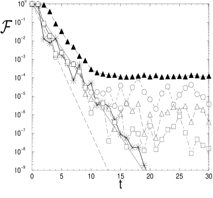
Figure 1: Decay of the fidelity ${\cal F}$ for the kicked rotor model with $K=10$, perturbation strength $\epsilon/\hbar=1.1$, $\hbar=3.1\times 10^{-3}$ (circles), $7.7\times 10^{-4}$ (empty triangles), and $1.9\times 10^{-4}$ (squares). Full triangles show the average fidelity $\overline{F}$ for $\hbar=7.7\times 10^{-4}$. Stars give the decay of the classical angular correlation function. The straight lines denote exponential decay with rates given by the Lyapunov exponent $\Lambda\approx\ln(K/2)=1.61$ (dashed line) and by the exponent $\Lambda_{1}\equiv\tau_{c}^{-1}=1.1$ Silvestrov (2002) (solid line).

Note that the expected saturation values of $\overline{F}$ and ${\cal F}$ are $1/N$ and $1/(NM)$, respectively, where $N$ is the number of states in the Hilbert space and $M$ is the number of quantum cells inside the area $\Delta$. This expectation is a consequence of the randomization of phases of fidelity amplitudes and is borne out by the numerical data shown in Fig. 1.

VII Conclusions

In this paper we have demonstrated that the decay of the quantum fidelity ${\cal F}$, when the initial state is a fully incoherent mixture, is determined by the decay of a classical correlation function, which is totally unrelated to quantum phases. We point out that the classical autocorrelation function in Eq. (14) reproduces not only the slope but also the overall decay of the function ${\cal F}$. The classical dynamical variable that appears in this autocorrelation function depends on the form of the perturbation. Therefore the echo decay, even in a classically chaotic system in the semiclassical regime and with quantally strong perturbations, is to some extent perturbation-dependent. The quantum dephasing described in this paper is a consequence of internal dynamical chaos and takes place in absence of any external environment. We may therefore conclude that the underlying internal dynamical chaos produces a dephasing effect similar to the decoherence due to the environment.

VIII Acknowledgements

We are grateful to Tomaž Prosen and Dima Shepelyansky for useful discussions. This work was supported in part by EU (IST-FET-EDIQIP), NSA-ARDA (ARO contract No. DAAD19-02-1-0086) and the MIUR-PRIN 2005 “Quantum computation with trapped particle arrays, neutral and charged”. V.S. acknowledges financial support from the RAS Joint scientific program ”Nonlinear dynamics and solitons”.

References

- (1)
- (2) F.Haake, Quantum signatures of chaos (2nd. Ed.), Springer–Verlag (2000).
- (3) G. Casati and B.V. Chirikov (Eds.), Quantum chaos: between order and disorder, Cambridge University Press (1995).
- (4) M. C. Gutzwiller, Chaos in classical and quantum mechanics, Springer–Verlag (1991).
- Peres (1984) A. Peres, Phys. Rev. A 30, 1610 (1984).
- Prosen (2002) T. Prosen, and M. Žnidarič, J. Phys. A 35, 1455 (2002).
- Jalabert (2001) R. A. Jalabert, and H. M. Pastawski, Phys. Rev. Lett. 86, 2490 (2001).
- Jacquod (2001) Ph. Jacquod, P. G. Silvestrov, and C. W. J. Beenakker, Phys. Rev. E 64, 055203(R) (2001).
- Cerruti (2002) N. R. Cerruti, and S. Tomsovic, Phys. Rev. Lett. 88, 054103 (2002).
- (10) G. Benenti and G. Casati, Phys. Rev. E 65, 066205 (2002).
- Silvestrov (2002) P.G. Silvestrov, J. Tworzydło, and C. W. J. Beenakker, Phys. Rev. E 67, 025204(R) (2003).
- Vanicek (2003) J. Vaníček, and E.J. Heller, Phys. Rev. E 68, 056208 (2003); J. Vaníček, Phys. Rev. E 70, 055201(R) (2004).
- Cucchietti (2003) F. M. Cucchietti, D. A. R. Dalvit, J. P. Paz, and W. H. Zurek, Phys. Rev. Lett. 91, 210403 (2003).
- (14) W.G. Wang, G. Casati, and B. Li, Phys. Rev. E 69, 025201(R) (2004).
- (15) B. Eckhardt, J. Phys. A 36, 371 (2003).
- Benenti et al. (2003) G. Benenti, G. Casati, and G Veble, Phys. Rev. E 67, 055202(R) (2003).
- (17) S.A. Gardiner, J.I. Cirac, and P. Zoller, Phys. Rev. Lett. 79, 4790 (1997).
- (18) S. Schlunk, M.B. d’Arcy, S.A. Gardiner, D. Cassettari, R.M. Godun, and G.S. Summy, Phys. Rev. Lett. 90, 054101 (2003).
- (19) M.F. Andersen, A. Kaplan, and N. Davidson, Phys. Rev. Lett. 90, 023001 (2003); M.F. Andersen, A. Kaplan, T. Grünzweig, and N. Davidson, quant-ph/0404118.
- (20) S. Montangero, A. Romito, G. Benenti, and R. Fazio, Europhys. Lett. 71, 893 (2005).
- (21) S.M. Hammel, J.A. Yorke, and C. Grebogi, J. Complex. 3, 136 (1987).
- Sokolov (1984) V.V. Sokolov, Teor. Mat. Fiz. 61, 128 (1984); Sov. J. Theor. Math. 61, 1041 (1985).
- (23) The fidelity for a pure coherent initial state was computed by A. Iomin, Phys. Rev. E 70, 026206 (2004). In that paper, however, a random Gaussian perturbation was considered instead of a deterministic one.
- Miller (2001) M. H. Miller, J. Phys. Chem. A 105, 2942 (2001).
- Glauber (1963) R. J. Glauber, Phys. Rev. Lett. 10, 84 (1963).
- (26) R.Z. Sagdeev, D.A. Usikov, and G.M. Zaslavsky, Nonlinear Physics, Harwood Acdemic Publishers (1988), p. 207.
- (27) F.M. Izrailev, Phys. Rep. 196, 299 (1990).
- (28) F.L. Moore, J.C. Robinson, C.F. Barucha, B. Sundaram, and M.G. Raizen, Phys. Rev. Lett. 75, 4598 (1995).
- (29) J. Ringot, P. Szriftgiser, J.C. Garreau, and D. Delande, Phys. Rev. Lett. 85, 2741 (2000).
- (30) H. Ammann, R. Gray, I. Shvarchuck, and N. Christensen, Phys. Rev. Lett. 80, 4111 (1998).
- (31) M.B. d’Arcy, R.M. Godun, M.K. Oberthaler, D. Cassettari, and G.S.Summy, Phys. Rev. Lett. 87, 074102 (2001).
- (32) M. Bienert, F. Haug, W.P. Schleich, and M.G. Raizen, Phys. Rev. Let.. 89, 050403 (2002).
- (33) F. Haug, M. Bienert, W.P. Schleich, T.H. Seligman, and M.G. Raizen, Phys. Rev. A 71, 043803 (2005).