Quantum random walk of the field in an externally driven cavity

Abstract

Using resonant interaction between atoms and the field in a high quality cavity, we show how to realize quantum random walks as proposed by Aharonov et al [Phys. Rev. A 48, 1687 (1993)]. The atoms are driven strongly by a classical field. Under conditions of strong driving we could realize an effective interaction of the form $iS^{x}(a-a^{{\dagger}})$ in terms of the spin operator associated with the two level atom and the field operators. This effective interaction generates displacement in the field’s wavefunction depending on the state of the two level atom. Measurements of the state of the two level atom would then generate effective state of the field. Using a homodyne technique, the state of the quantum random walker can be monitored.

I Introduction

In a very interesting paper Aharonov et al Aharonov proposed the idea of a quantum random walk. Here a random walker is constrained to move left or right depending on the state of an auxiliary quantum mechanical system. One then examines the state of the random walker subject to the measurement of the state of the auxiliary system. As an interesting consequence of this quantum random walk, Aharonov et al Aharonov found that the walker’s distribution could shift by an amount which could be larger than the width of the initial distribution. Further the displacement could be much larger than the classical displacement. Several proposals Cavity ; Aharonov ; Sanders ; milburn ; lattice ; exp ; knight ; bouwmeester exist for realizations of the quantum random walk. For example Aharonov et al gave a cavity QED model where the photon number distribution can get displaced. Sanders et al Sanders considered a dispersive interaction in the cavity of the form $S^{z}(a+a^{{\dagger}})$ and considered the random walk of the field on states on a circle. Other interesting theoretical schemes for implementing quantum walks have been suggested in ion-traps milburn and in optical lattices lattice . Knight et al knight further showed that an earlier experiment bouwmeester was a realization of quantum random walks. A scheme using linear optical elements has been recently implemented exp .

Here we propose a method which yields precisely quantum random walk as proposed by Aharonov et al. We use cavity QED however we drive the atoms by an external field. Currently there is considerable progress in realizing a variety of high quality cavities and a variety of interactions and thus one is in a situation where proposals like the one presented here are likely to be implemented.

The organization of the paper is as follows. In Sec.II we present the details of our model and show the conditions under which such a model gives rise to an effective Hamiltonian which we use in Sec.III to realize quantum random walk. In this section we also present the results for the Wigner function for the state of the quantum walker. In Sec.IV we show how the homodyne measurements of the field can be used to check the characteristics of the quantum random walk. In Sec.V we incorporate the effects of decoherence due to the decay of the field in the cavity. In the appendix we discuss the state of the walker if no conditional measurements are made and establish relation to classical random walks.

II Effective hamiltonian for Quantum Random Walk using driven atoms

We consider a two level Rydberg atom having its higher energy state $|e\rangle$ and lower energy state $|g\rangle$, interacting with a single mode of the electromagnetic field in a cavity. The atom passes through the cavity and interacts resonantly with the field. Further the atom is driven by a strong classical field. For simplicity we choose atomic transition frequency, the cavity frequency and the frequency of the driving field to be same. The Hamiltonian for the system in the interaction picture is written as

$$H=-i\hbar g\left(S^{+}a-a^{{\dagger}}S^{-}\right)+\hbar\left(S^{+}{\cal{E}}+S^{-}{\cal{E}}^{*}\right),$$ (1)

where $g$ and ${\cal{E}}$ are the coupling constants of the interaction of the atom with the cavity field and with the deriving field. We have chosen $g$ as real and ${\cal{E}}$ as complex. The annihilation (creation) operator for the field in the cavity is $a(a^{{\dagger}})$ and $S^{+},~{}S^{-}$ are atomic spin operators. The last term in Eq.(1) is the interaction with the external field. We further rewrite the above Hamiltonian in a picture in which the interaction with the external field has already been diagonalized.

$$|\bar{\psi}\rangle=e^{iht}|\psi\rangle;~{}h=S^{+}{\cal{E}}+S^{-}{\cal{E}}^{*},$$ (2)

where $|\bar{\psi}\rangle$ is transformed atomic state in new picture from old atomic state $|\psi\rangle$. The Hamiltonian in this picture is

$$\bar{H}=-ige^{iht}(S^{+}a-S^{-}a^{{\dagger}})e^{-iht},$$ (3)

$$e^{iht}\equiv\cos(|{\cal{E}}|t)+\frac{ih}{|{\cal{E}}|}\sin(|{\cal{E}}|t).$$ (4)

The atomic spin operators $S^{\pm}$ transform as

$$e^{iht}S^{+}e^{-iht}\equiv S^{+}\cos^{2}(|{\cal{E}}|t)+\frac{{\cal{E}}^{*2}}{|{\cal{E}}|^{2}}\sin^{2}(|{\cal{E}}|t)S^{-}$$

$$-\frac{2i{\cal{E}^{*}}}{|{\cal{E}}|}S^{z}\sin(|{\cal{E}}|t)\cos(|{\cal{E}}|t),$$ (5)

$$e^{iht}S^{-}e^{-iht}\equiv S^{-}\cos^{2}(|{\cal{E}}|t)+\frac{{\cal{E}}^{2}}{|{\cal{E}}|^{2}}\sin^{2}(|{\cal{E}}|t)S^{+}$$

$$+\frac{2i{\cal{E}}}{|{\cal{E}}|}S^{z}\sin(|{\cal{E}}|t)\cos(|{\cal{E}}|t).$$ (6)

Using Eqs.(II) and (II), Eq.(3) becomes

$$\bar{H}=-ig\left(S^{+}\cos^{2}(|{\cal{E}}|t)+\frac{{\cal{E}}^{*2}}{|{\cal{E}}|^{2}}\sin^{2}(|{\cal{E}}|t)S^{-}\right.$$

$$\left.-\frac{2i{\cal{E}^{*}}}{|{\cal{E}}|}S^{z}\sin(|{\cal{E}}|t)\cos(|{\cal{E}}|t)\right)a-H.c.$$ (7)

We note that the Hamiltonians of the above form have been previously used to treat the inhibition of the spontaneous emission spe and for the production of Schrodinger cat states Solano . We assume that the atom is driven strongly so that $|{\cal{E}}|$ is large and hence we drop rapidly oscillating terms from Eq.(7) i.e. $e^{\pm 2i|{\cal{E}}|t}\Rightarrow 0$. Then Eq.(7) reduces to

$$\bar{H}=-\frac{ig}{2}\left(S^{+}+\frac{{\cal{E}}^{*2}}{|{\cal{E}}|^{2}}S^{-}\right)a-H.c.$$ (8)

We choose ${\cal{E}}^{*2}/{|\cal{E}}|^{2}=1$, in general, this can also be done by adjusting phases with atomic operators. Then the Eq.(8) takes the form

$$\bar{H}_{eff}=gS^{x}\left(\frac{a-a^{{\dagger}}}{i}\right).$$ (9)

Note the appearance of the well known displacement $D(\alpha)=(a^{{\dagger}}\alpha-a\alpha^{*})$ in the Eq.(9). In particular we have the momentum operator (out of phase quadrature for the field). Further it should also be noted that $h$ as defined by Eq.(2) commutes with $\bar{H}_{eff}$. In the original interaction picture the Hamiltonian for our model will be

$$H_{eff}=gS^{x}\left(\frac{a-a^{{\dagger}}}{i}\right)+2|{\cal{E}}|S^{x}.$$ (10)

In the effective Hamiltonian (10) field displacement operator appears with atomic operator, which can produce displacement in field state depending on the atomic state.

III realization of random walk

We next examine the evolution of the system of the two level atom and the field inside the cavity. Let us consider that, initially the atom is in the superposition state $|\Phi\rangle=(c_{1}|e\rangle+c_{2}|g\rangle)$ and the field is in a coherent state $|\alpha\rangle$. Using Eq.(10) the combined state of the atom-cavity system after time $t$ is given by

$$|\psi(t)\rangle = \exp\left[gtS^{x}(a^{{\dagger}}-a)-2i|{\cal{E}}|tS^{x}\right]|\Phi\rangle|\alpha\rangle,$$

$$= \frac{c_{+}e^{-i\phi}}{2}\left(|g\rangle+|e\rangle\right)|\alpha+gt/2\rangle$$

$$+ \frac{c_{-}e^{i\phi}}{2}\left(|g\rangle-|e\rangle\right)|\alpha-gt/2\rangle,$$

$$= |g\rangle\left[\frac{c_{+}e^{-i\phi}}{2}|\alpha+gt/2\rangle+\frac{c_{-}e^{i\phi}}{2}|\alpha-gt/2\rangle\right]$$

$$+ |e\rangle\left[\frac{c_{+}e^{-i\phi}}{2}|\alpha+gt/2\rangle-\frac{c_{-}e^{i\phi}}{2}|\alpha-gt/2\rangle\right];$$ (13)

$$\phi = \left(|{\cal{E}}|+\frac{g}{2}Im(\alpha)\right)t;$$ (14)

where $c_{+}=c_{1}+c_{2}$ and $c_{-}=c_{1}-c_{2}$. Using normalization of atomic states we can select $c_{-}/c_{+}=\tan\theta$. Thus the detection of the atom in state $|e\rangle$ or $|g\rangle$ leaves the cavity field in a superposition of states $|\alpha+gt/2\rangle$ and $|\alpha-gt/2\rangle$. For small values of $gt$ the states $|\alpha+gt/2\rangle$ and $|\alpha-gt/2\rangle$ overlap completely and thus quantum interference effects between $|\alpha+gt/2\rangle$ and $|\alpha-gt/2\rangle$ becomes significant. If we assume that the atom is detected in its ground state $|g\rangle$. Then the state of the field inside the cavity can be written as

$$|\psi_{f}\rangle\propto\left[e^{-i|{\cal{E}}|t}D(gt/2)+e^{i|{\cal{E}}|t}\tan(\theta)D(-gt/2)\right]|\alpha\rangle,$$ (15)

Clearly after passing one atom through the cavity the field inside the cavity is displaced backward or forward along the line in a random way by the step of $gt/2$. We can now iterate the above step to obtain the state of the field after the passage of $N$ atoms. We assume that atoms enter in the cavity in the state $|\Phi\rangle$ and after interaction with the field inside the cavity detected in their ground state $|g\rangle$. Note that the displacement operators appearing in the above state commute each other $[D(gt/2),D(-gt/2)]=0$ for real $gt$. Thus the field state after the passage of $N$ atoms is given by

$$|\psi_{f}(N)\rangle = C\left[e^{-i|{\cal{E}}|t}D(gt/2)+e^{i|{\cal{E}}|t}\tan(\theta)D(-gt/2)\right]^{N}|\alpha\rangle,$$

$$= C\sum_{m=0}^{N}\left(\begin{array}[]{c}N\\ m\\ \end{array}\right)\left[e^{-im|{\cal{E}}|t}D^{m}\left(\frac{gt}{2}\right)\times\right.~{}~{}~{}~{}~{}~{}~{}~{}$$

$$\left.e^{i(N-m)|{\cal{E}}|t}(\tan\theta)^{N-m}D^{N-m}\left(-\frac{gt}{2}\right)\right]|\alpha\rangle,$$

$$= C\sum_{m=0}^{N}\left(\begin{array}[]{c}N\\ m\\ \end{array}\right)e^{i(N-2m)|{\cal{E}}|t}(\tan\theta)^{N-m}$$ (22)

$$D^{N-2m}(-gt/2)|\alpha\rangle,$$

$$= C\sum_{m=0}^{N}\left(\begin{array}[]{c}N\\ m\\ \end{array}\right)e^{i(N-2m)\phi}(\tan\theta)^{N-m}$$ (26)

$$|\alpha-(N-2m)gt/2)\rangle,$$

where $C$ is normalization constant and we have used the property of the displacement operator $D^{-1}(\alpha)=D(-\alpha)$. On writing the above result in coordinate space representation, we get the wavefunction $\psi_{N}(x,\alpha)=\langle x|\psi_{f}(N)\rangle$

$$\psi_{N}(x,\alpha)=C\sum_{m=0}^{N}\left(\begin{array}[]{c}N\\ m\\ \end{array}\right)e^{i(N-2m)\phi}(\tan\theta)^{N-m}$$ (29)

$$\psi_{\alpha}\left(x+[N-2m]l\right),$$ (30)

where $\psi_{\alpha}(x)\equiv\langle x|\alpha\rangle$ is the wavefunction corresponding to the initial cavity field state $|\alpha\rangle$ which is centered at $x=\alpha$ and the step size of the random walker is $l=gt/2$. We note that we have recovered the result of Aharonov et al Aharonov . In Fig.1 we have plotted the probability amplitude distribution for initial wave function $\psi_{\alpha}(x)\sim\exp[-(x-\alpha)^{2}/2]$ for real values of $x$ and $\alpha=0$. The displacement depends on $\theta$, $\phi$ and the number of steps $N$. The unexpected displacement in the state of the random walker is the result of constructive quantum interference between the states generated in various steps which comes from the off diagonal terms in $P(x)=|\psi_{N}(\alpha,x)|^{2}$. We have checked this by dropping the off diagonal terms in $P(x)$, in that case $P(x)$ remains same in shape as the initial wave packet but shifts by an amount $Nl$. The displacement of the random walker is not bounded by the classically possible maximum and minimum displacements $\pm Nl$. The quantum interference leads to an arbitrary displacement in the random walker’s position and can be much larger than $\pm Nl$. A small squeezing in wavepacket is also generated from these interference effects. The selection of phase $\phi$ is also critical for displacement in the position of quantum walker, for example for the parameters used in Fig.1 the maximum displacement in the position of quantum walker occurs when $\phi$ is integer multiple of $\pi$ and there will be minimum displacement when $\phi$ is half integer multiple of $\pi$.

Figure 1: The probability distribution $P(x)$ for the position of the quantum random walker, assuming initial wave packet as Gaussian $\exp[-(x-\alpha)^{2}/2]$ for $\alpha=0$, step size $l=0.05$, $\phi=2\pi$ and $\theta=2\pi/3$.

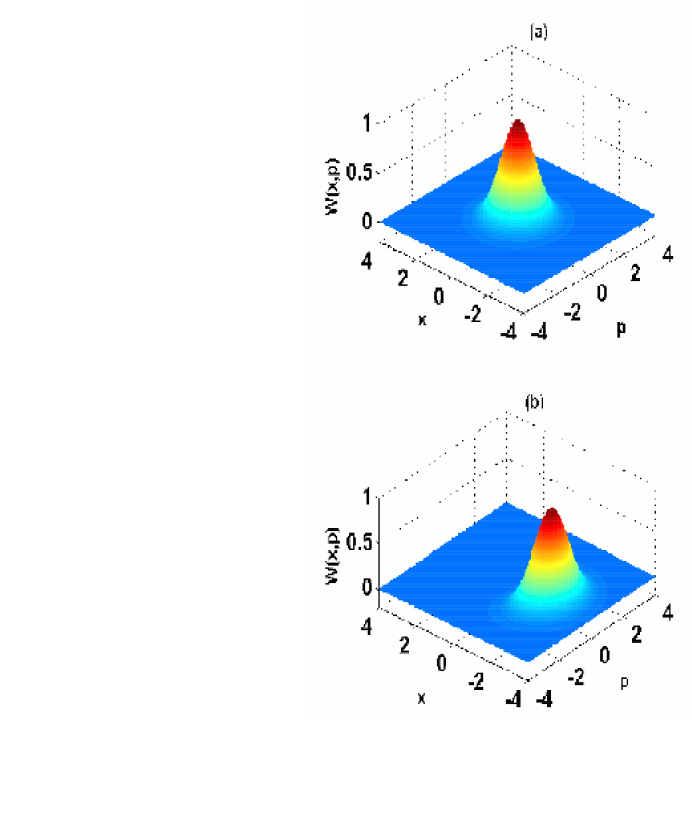
Figure 2: The Wigner function $W(x,p)$ of the state of the random walker, after number of steps (a) $N=0$ (b) $N=10$, using same parameters as in FIG.1.

For visualizing quantum interferences we plot the Wigner function of the random walker in Fig.2. The Wigner distribution for any state $\psi(x)$ can be obtained by using the definition wigner ,

$$W(x,p)=\frac{1}{\pi\hbar}\int e^{2ipy/\hbar}\psi(x-y)\psi^{*}(x+y)dy.$$ (31)

In the Fig.2(a) the field is in its initial coherent state and the wigner function is perfect Gaussian. As the field is displaced by random steps, by passing atoms through the cavity, quantum interference effects start deforming the shape of the Wigner function from the Gaussian. After few steps the Wigner function is squeezed in $x$ quadrature and gets displaced by an arbitrary distance in $x$. In Fig.2(b), (see also Fig.4(a)), we have shown the Wigner function after $10$ random steps for initial Gaussian wave packet. The squeezing is also clear from the Fig.1 which shows the narrowing of the distribution $P(x)$. It is clear that the displacement in the position of random walker comes as a result of quantum interference which is consequence of quantum coherence between the states generated in random steps.

IV measurement of the state of the random walker

We next discuss how we can probe the quantum state of the random walker. We propose homodyne techniques homodyne for measuring the state of the random walker. Such homodyne measurement can be performed by mixing an external resonant coherent field to the cavity and then probing the resultant cavity field by passing a test atom through the cavity. In the previous section, we have shown how the cavity field is displaced backward or forward in a random step by passing single atom through the cavity. The state of the field in the cavity after such $N$ steps can be monitored by homodyne measurements which can be implemented in the same experimental set up. After displacing the field inside the cavity by $N$ random steps, by passing $N$ atoms, a resonant external coherent field $|\beta\rangle$ is injected into the cavity. After adding the external field, the state of the resultant field in the cavity is

$$|\psi_{H}\rangle = C\sum_{m=0}^{N}\left(\begin{array}[]{c}N\\ m\\ \end{array}\right)e^{i(N-2m)\phi}(\tan\theta)^{N-m}$$

$$D(\beta)|\alpha-(N-2m)gt/2)\rangle,$$

$$= C\sum_{n}\sum_{m=0}^{N}\left(\begin{array}[]{c}N\\ m\\ \end{array}\right)e^{i(N-2m)\phi}(\tan\theta)^{N-m}$$

$$\langle n|D(\beta)|\alpha-(N-2m)gt/2)\rangle|n\rangle,$$

$$= \sum_{n}F_{n}|n\rangle$$ (38)

$$F_{n} = C\sum_{m=0}^{N}\left(\begin{array}[]{c}N\\ m\\ \end{array}\right)e^{i(N-2m)\phi}(\tan\theta)^{N-m}$$ (42)

$$\langle n|D(\beta)|\alpha-(N-2m)gt/2)\rangle.$$

Now we bring a similar atom in its lower energy state $|g\rangle$ to probe the cavity field. The probability of detecting the probe atom in its lower state $|g\rangle$ after crossing the cavity in time $t_{p}$ is

$$P_{g}=\sum_{n}|F_{n}|^{2}\cos^{2}(gt_{p}\sqrt{n}).$$ (43)

The interaction time $t_{p}$ for the probe atom is selected such that if there are photons in the cavity it leaves the cavity in its higher energy state $|e\rangle$ with larger probability. If we choose the external field $|\beta\rangle$ such that $\beta=-\alpha+\delta$, the probe atom will leave the cavity in its ground state with larger probability when the value of $\delta$ will be opposite and equal to the displacement of the random walker from the initial position $\alpha$. Thus the probability of the probe atom leaving the cavity in its lower state $|g\rangle$ would, as a function of $\delta$, have peak corresponding to the positions of the random walker after $N$ steps. In Fig.3, we plot the probability of detecting the probe atom in its lower state with $\delta$. The solid line curve is result of homodyne measurement of the position of the random walker corresponding to its initial state. The dashed line curve is corresponding to the homodyne measurement after $10$ steps using the same parameter as in Fig.1. Clearly the homodyne measurement yields the state of the quantum walker (Fig.1). Thus the homodyne measurement can be an elegant way for monitoring the position of the random walker in our model of realizing quantum random walks.

Figure 3: The probability of detecting probe atom in its ground state as a function of $\delta$ for the state of the quantum random walker after number of steps $N=0$ ( solid line) and $N=10$ (dashed line). The parameters used are same as in Fig.1 and the interaction time for the probe atom is selected such that $gt_{p}=1.5\pi$.

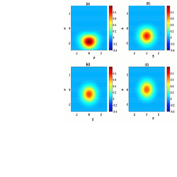
Figure 4: The decoherence of the state of the random walker in terms of Wigner function at different times, (a) for $\kappa t=0$, (b) for $\kappa t=1/4N^{2}l^{2}$, (c) for $\kappa t=1/2N^{2}l^{2}$, (d) for $\kappa t=2/N^{2}l^{2}$, other parameters are same as FIG.2 (b).

V decoherence of the generated state of the random walker

Quantum random walks are different from the classical random walks in the sense of quantum interferences which may lead much larger displacements in the position of quantum random walker than the classically possible maximum displacements. These quantum interferences are the consequences of coherence in the system. Clearly we need the coherence to live for a long time and thus it is important to study the effects of the decoherence of the system. In this section we study the decoherence of the state of the random walker due to damping in the cavity. This can be done using the master equation

$$\dot{\rho}=-\frac{\kappa}{2}(a^{{\dagger}}a\rho-2a\rho a^{{\dagger}}+\rho a^{{\dagger}}a),$$ (44)

where $\kappa$ is cavity field decay parameter and we carry analysis in the absence of thermal photons. For initial state (26) we find the density matrix after time $t$

$$\rho(t) = |C|^{2}\sum_{m=0}^{N}\sum_{n=0}^{N}\left(\begin{array}[]{c}N\\ m\\ \end{array}\right)\left(\begin{array}[]{c}N\\ n\\ \end{array}\right)e^{2i(n-m)\phi}(\tan\theta)^{2N-m-n}$$ (50)

$$\langle\alpha-(N-2m)l|\alpha-(N-2n)l)\rangle^{(1-e^{-\kappa t})}$$

$$|\alpha-(N-2m)l\rangle_{t}\langle\alpha-(N-2n)l|_{t}~{},$$

where $|\zeta\rangle_{t}\equiv|\zeta e^{-\kappa t/2}\rangle$. In the limit $\kappa t<<1$ the Eq.(50) simplifies to

$$\rho(t) = |C|^{2}\sum_{m=0}^{N}\sum_{n=0}^{N}\left(\begin{array}[]{c}N\\ m\\ \end{array}\right)\left(\begin{array}[]{c}N\\ n\\ \end{array}\right)e^{2i(n-m)\phi}(\tan\theta)^{2N-m-n}$$ (56)

$$e^{-2\kappa tl^{2}(n-m)^{2}}|\alpha-(N-2m)l\rangle\langle\alpha-(N-2n)l|.$$

Thus the coherence of the state decays on the time scales $1/2N^{2}l^{2}$. In Fig.4 we show the decoherence effects due to the cavity damping in the state of the quantum random walker in terms of Wigner function. As the time progresses from (a) to (d) the decoherence reduces the quantum interference effects and the state of the random walker decays to its initial state. In Fig.4(a) the Wigner function for the state of the random walker after $10$ steps using the parameters of Fig.2(b) is plotted which is squeezed in $x$ quadrature and centered at $x\approx-2$. As a result of decoherence due to cavity damping the quantum interferences start decaying and the Wigner function changes to the perfect Gaussian shape, Fig.4(c) centered at $x=Nl$. Now the field inside the cavity is almost in coherent state and decays with the cavity damping rate. Further the life time for the state of the quantum random walker is given by $T_{N}=T_{c}/2N^{2}l^{2}$ where $T_{c}=1/\kappa$ is life time for field in the cavity.

VI conclusions

In conclusion we have shown a simple possible realization of quantum random walks using cavity QED. We have proposed homodyne detection for monitoring the position of the random walker. We have also discussed the decoherence effects and the time scales at which quantum nature of random walks survives. As a result of new emerging technologies various improved cavities are feasible these days cavity , which makes our proposal much interesting and realistic. Such realization of quantum random walks may be useful for implementing various algorithms algorithms based on quantum random walks. Finally it should be noted that the generalizations of the present work to more than one dimensions are possible. *

Appendix A State of the walker for no measurement on the atomic state

In this appendix we would like to connect the result (III) explicitly to the case of classical random walk. For this purpose we find the reduced state of the field from (III). We also set $c_{1}=1,~{}c_{2}=0$, then the reduced state of the field $\rho_{f}$ is

$$\rho_{f}=\frac{1}{2}\left(|\alpha+\frac{gt}{2}\rangle\langle\alpha+\frac{gt}{2}|+|\alpha-\frac{gt}{2}\rangle\langle\alpha-\frac{gt}{2}|\right)$$ (57)

Clearly the state of the field after the passage of $N$ atoms would be

$$\rho_{f}=\left(\frac{1}{2}\right)^{N}\sum_{m=0}^{N}\left(\begin{array}[]{c}N\\ m\\ \end{array}\right)\times~{}~{}~{}~{}~{}~{}~{}~{}~{}~{}~{}~{}~{}~{}~{}~{}~{}~{}~{}$$ (60)

$$|\alpha+\frac{gt}{2}(N-2m)\rangle\langle\alpha+\frac{gt}{2}(N-2m)|$$ (61)

$$=\left(\frac{1}{2}\right)^{N}\sum_{p=-N}^{+N}\frac{N!}{\frac{N-p}{2}!\frac{N+p}{2}!}|\alpha+\frac{gt}{2}p\rangle\langle\alpha+\frac{gt}{2}p|$$ (62)

which is reminiscent of the result for classical random walk in the sense that the weight factor of the state $|\alpha+\frac{gt}{2}p\rangle\langle\alpha+\frac{gt}{2}p|$ is same as the probability of finding the walker at the site $p$ chandra . It should however be borne in mind that the coherent states $|\alpha+\frac{gt}{2}p\rangle$ and $|\alpha+\frac{gt}{2}p^{\prime}\rangle$ are not orthogonal for $p\neq p^{\prime}$.

References

- (1) Y. Aharonov, L. Davidovich, and N. Zagury, Phys. Rev. A 48, 1687 (1993).
- (2) B. C. Sanders, S. D. Bartlett, B. Tregenna, and P. L. Knight, Phys. Rev. A 67, 042305 (2003).
- (3) T. Di, M. Hillery, and M. S. Zubairy, Phys. Rev. A 70, 032304 (2004).
- (4) B. C. Travaglione and G. J. Milburn, Phys. Rev. A 65, 032310 (2002).
- (5) W. Dür, R. Raussendorf, V. M. Kendon, and H. -J. Briegel, Phys. Rev. A 66, 052319 (2002); K. Eckert, J. Mompart, G. Birkl, M. Lewenstein, e-print quant-ph/0503084.
- (6) P. L. Knight, E. Roldan, and J. E. Sipe, Phys. Rev. A 68, 020301(R) (2003); Opt. Commun. 227, 147 (2003).
- (7) D. Bouwmeester, I. Marzoli, G. P. Karman, W. Schleich, and J. P. Woerdman, Phys. Rev. A 61, 013410 (2000).
- (8) B. Do, M. L. Stohler, S. Balasubramanian, D. S. Elliott, C. Eash, E. Fischbach, M. A. Fischbach, A. Mills, B. Zwickl, J. Opt. Soc. Am. B, 22, 499 (2005); H. Jeong, M. Paternostro, and M. S. Kim, Phys. Rev. A 69 , 012310 (2004).
- (9) G. S. Agarwal, W. Lange, and H. Walther, Phys. Rev. A 48, 4555 (1993).
- (10) E. Solano, G. S. Agarwal, and H. Walther, Phys. Rev. Lett. 90, 027903 (2003).
- (11) M. Hillery, R. F. O’Connell, M. O. Scully, and E. P. Wigner, Phys. Rep. 106, 121(1984).
- (12) A. Auffeves,P. Maioli, T. Meunier, S. Gleyzes, G. Nogues, M. Brune, J. M. Raimond, and S. Haroche, Phys. Rev. Lett. 91, 230405 (2003).
- (13) M. Keller, B. Lange, K. Hayasaka, W. Lange, H. Walther, Nature (London) 431, 1075 (2004); P. Maunz, T. Puppe, I. Schuster, N. Syassen, P. W. H. Pinkse, G. Rempe, Nature (London) 428, 50 (2004).
- (14) N. Shenvi, J. Kempe, and K. BirgittaWhaley, Phys. Rev. A 67, 052307 (2003).
- (15) S. Chandrasekhar, Rev. Mod. Phys. 15, 1 (1943).