Limitations on the Utility of Exact Master Equations

Abstract

The low temperature solution of the exact master equation for an oscillator coupled to a linear passive heat bath is known to give rise to serious divergences. We now show that, even in the high temperature regime, problems also exist, notably the fact that the density matrix is not necessarily positive.

,

1 Introduction

In a previous publication [1], we presented a general solution of the exact master equation for an oscillator coupled to a linear passive heat bath. This was achieved by solving the generalized quantum Langevin equation for the initial value problem [2] which enabled us to obtain explicit expressions for the time-dependent coefficients occuring in the exact master equation. Mext, we illustrated the general solution with the construction of explicit expressions for the probability distributions for two examples: wave packet spreading and ”Schrödinger cat” state for a free particle. This enabled us to discover that the low temperature solution gave rise to divergences. The purpose of the present paper is to show that problems also exist in the high temperature regime. Thus, we are motivated to extend our previous analysis to obtain explicit expressions for the Wigner function and the elements of the density matrix, and with the aid of these results to critically examine the equation and its solution.

At the outset we must point out that the exact master equation has drawbacks that seriously limit its utility. For the most part these are related to the fact that the initial state is necessarily one in which the particle and heat bath are uncoupled, while the subsequent motion is described by the fully coupled system. The most serious of these is that the equation (and therefore its solution) has an irreparable divergence, irreparable in the sense that it persists in a cut-off model with finite bath relaxation time [1]. We believe this divergence is related to a well known phenomenon of quantum field theory: the Hilbert space spanned by the eigenfunctions of the coupled Hamiltonian is orthogonal to that of the uncoupled Hamiltonian [3]. It can be shown that this is the case for the system of coupled oscillators that is the microscopic basis for the derivation of the exact master equation and its solution [4, 5].

The exception is the high temperature limit, where the divergence does not appear since, by convention, one there neglects the zero-point oscillations of the bath. We therefore confine our discussion to that limit. However, even in that case there are further difficulties. The first of these is that the initial state breaks the translational invariance of the system. This is manifest in an initial squeeze centered at the origin that, for a free particle, results in a drift of the mean position toward the origin. For this reason in the examples we consider only the case of a free particle, where this difficulty is most apparent.

A second difficulty with the equation in the high temperature limit is that for short times the diagonal elements of the density matrix, which have the physical interpretation of probabilities, are not necessarily positive. This is a well known difficulty with the weak coupling master equation, solved by a further time average to bring it to the so-called Lindblad form that guarantees positivity [6]. It was supposed that the exact master equation, with its time-dependent coefficients, would be immune but, as we shall show explicitly, in the high temperature limit this difficulty remains. The situation, therefore, is that there are concerns that seriously limit the utility of the exact master equation. The irreparable divergence can only be avoided with the neglect of zero-point oscillations in the high temperature limit, and even there problems remain with the failure of translational invariance and positivity.

Despite these problems, we argue that the solution of the exact master equation can be useful. In particular, we show that when the initial particle temperature is taken to be equal to that of the bath, we obtain results that for short times are identical with those obtained  from a calculation which considers entanglement at all times [7]. Finally, an important result is the demonstration that measures of decoherence based on the Wigner function are identical with those based on the off-diagonal elements of the density matrix. We argue that the Wigner function, being everywhere real, is the preferable description.

2 General solution in high temperature limit

The exact master equation, in terms of the Wigner function $W(q,p,t)$ for the complete system of oscillator plus heat bath, may be expressed in the form

$$\frac{\partial W}{\partial t} = -\frac{1}{m}p\frac{\partial W}{\partial q}+m\Omega^{2}(t)q\frac{\partial W}{\partial p}$$ (1)

$${}+2\Gamma(t)\frac{\partial pW}{\partial p}+\hbar m\Gamma(t)h(t)\frac{\partial^{2}W}{\partial p^{2}}+\hbar\Gamma(t)f(t)\frac{\partial^{2}W}{\partial q\partial p},$$

and we note the presence of four time-dependent coefficients for which we obtained explicit expressions [1].

The general solution of the exact master equation is most simply expressed in terms of the Wigner characteristic function (the Fourier transform of the Wigner function).

$$\tilde{W}(Q,P;t)=\int dq\int dpe^{-i(qP+pQ)/\hbar}W(q,p;t).$$ (2)

Expressed in terms of this function, the general solution given in Eq. (4.15) of [1] takes the simple form,

$$\tilde{W}(Q,P;t) = \exp\{-\frac{\left\langle X^{2}\right\rangle P^{2}+m\left\langle X\dot{X}+\dot{X}X\right\rangle QP+m^{2}\left\langle\dot{X}^{2}\right\rangle Q^{2}}{2\hbar^{2}}\}$$ (3)

$$\times\tilde{W}(m\dot{G}Q+GP,m^{2}\ddot{G}Q+m\dot{G}P;0).$$

In this expression $X(t)$ is the fluctuating position operator, defined in Eq. (2.16) of [1], while $G(t)$ is the Green function, defined in general to be

$$G(t_{2}-t_{1})=\frac{1}{i\hbar}[x(t_{1}),x(t_{2})]\theta(t_{2}-t_{1}),$$ (4)

in which $x(t)$ is the time-dependent Heisenberg coordinate operator and $\theta$ is the Heaviside function.

It was shown in [1] (Sec. V.A.2) that the quadratic expectations $\left\langle X^{2}\right\rangle$, $\left\langle X\dot{X}+\dot{X}X\right\rangle$ and $\left\langle\dot{X}^{2}\right\rangle$ are logarithmically divergent, which has the effect that the solution (3) vanishes identically for non-zero positive times. There, too, it was shown that the divergence is irreparable, in the sense that it persists in a model with a high frequency cut-off. As was stated in the Introduction, it appears that this is a reflection of the well established fact that the states of the uncoupled system (the initial state) are orthogonal to those of the coupled system (states for later times) [4, 5]. This fact, surprising from the point of view of the quantum mechanics of finite systems, is a feature only of systems with an infinite number of degrees of freedom. In our case it is the heat bath that must be infinite. In any event, the upshot is that, while the derivation of the exact master equation is formally correct, there is no useful result. The exception is the high temperature limit, where by convention one neglects zero-point oscillations. We therefore restrict our further discussion to this limit. Indeed, it is this limit (or better said: approximation) that has been considered in all previous discussions of the exact master equation.

In considering the result in the high temperature limit, we restrict our discussion to the Ohmic model of coupling to the heat bath, which is adequate for our purposes. This model corresponds to Newtonian friction, with retarding force proportional to the velocity. In addition we consider only the case of a free particle, moving in the absence of any external potential. Choosing the friction constant to be $m\gamma$, the Green function then takes the simple form:

$$G(t)=\frac{1-e^{-\gamma t}}{m\gamma}.$$ (5)

In the high temperature limit the moments appearing in the solution can then be written in the form:

$$\left\langle X^{2}\right\rangle = 2m\gamma kT\int_{0}^{t}dt^{\prime}G^{2}(t^{\prime})$$

$$= \frac{kT}{m\gamma^{2}}[2\gamma t-(1-e^{-\gamma t})(3-e^{-\gamma t})],$$

$$\left\langle X\dot{X}+\dot{X}X\right\rangle = 2m\gamma kTG^{2}(t)$$

$$= \frac{2kT}{m\gamma}(1-e^{-\gamma t})^{2},$$

$$\left\langle\dot{X}^{2}\right\rangle = 2m\gamma kT\int_{0}^{t}dt^{\prime}\dot{G}^{2}(t^{\prime})$$ (6)

$$= \frac{kT}{m}(1-e^{-2\gamma t}).$$

We should emphasize that in these  expressions $T$ is the temperature of the bath. In the initial state the bath and the particle are uncoupled, so in the general solution (3) $\tilde{W}(Q,P;0)$, the initial Wigner characteristic function, may be chosen to have any form consistent with a single particle not coupled to a bath. In the examples we consider two possibilities: the particle initially at zero temperature and at a temperature equal to that of the bath.

3 Example: Gaussian wave packet

3.1 Initial particle temperature zero

We consider first an initial state corresponding to a Gaussian wave packet, with wave function of the form

$$\phi(x,0)=\frac{1}{(2\pi\sigma^{2})^{1/4}}\exp\{-\frac{(x-x_{0})^{2}}{4\sigma^{2}}\}.$$ (7)

This is a stationary wave packet, centered at $x_{0}$ with mean square width $\sigma^{2}$. It is a minimum uncertainty wave packet, since the mean square momentum has the minimum value $\hbar^{2}/4\sigma^{2}$. The corresponding Wigner characteristic function is

$$\tilde{W}(Q,P;0) = \int_{-\infty}^{\infty}dxe^{-iPx/\hbar}\phi(x-\frac{Q}{2},0)\phi^{\ast}(x+\frac{Q}{2},0)$$ (8)

$$= \exp\{-\frac{Q^{2}}{8\sigma^{2}}-\frac{\sigma^{2}P^{2}}{2\hbar^{2}}-i\frac{x_{0}P}{\hbar}\}.$$

This initial state is what is termed a pure state. The condition for a pure state is usually stated in terms of the density matrix: $\mathrm{Tr}\{\rho^{2}\}=1$. In terms of the Wigner characteristic function, this condition becomes

$$\frac{1}{2\pi\hbar}\int_{-\infty}^{\infty}dQ\int_{-\infty}^{\infty}dP\left|\tilde{W}(Q,P)\right|^{2}=1.$$ (9)

It is easy to show that a state is a pure state if and only if it can be associated to a wave function. Such a pure state necessarily corresponds to a particle at zero temperature; a finite-temperature state is a mixed state.

Putting the expression (8) for the initial Wigner characteristic function in the general solution (3) we see that

$$\tilde{W}(Q,P;t)=\exp\{-\frac{A_{11}^{(0)}P^{2}+2A_{12}^{(0)}PQ+A_{22}^{(0)}Q^{2}}{2\hbar^{2}}-i\frac{x_{0}(m^{2}\ddot{G}Q+m\dot{G}P)}{\hbar}\},$$ (10)

where we have introduced

$$A_{11}^{(0)} = \left\langle X^{2}\right\rangle+\sigma^{2}m^{2}\dot{G}^{2}+\frac{\hbar^{2}G^{2}}{4\sigma^{2}}$$

$$= \frac{kT}{m\gamma^{2}}[2\gamma t-(1-e^{-\gamma t})(3-e^{-\gamma t})]+\sigma^{2}e^{-2\gamma t}+\frac{\hbar^{2}(1-e^{-\gamma t})^{2}}{4m^{2}\gamma^{2}\sigma^{2}},$$

$$A_{12}^{(0)} = m\frac{\left\langle X\dot{X}+\dot{X}X\right\rangle}{2}+\sigma^{2}m^{3}\dot{G}\ddot{G}+\frac{\hbar^{2}mG\dot{G}}{4\sigma^{2}}$$

$$= \frac{kT}{\gamma}(1-e^{-\gamma t})^{2}-m\gamma\sigma^{2}e^{-2\gamma t}+\frac{\hbar^{2}(e^{-\gamma t}-e^{-2\gamma t})}{4m\gamma\sigma^{2}},$$

$$A_{22}^{(0)} = m^{2}\left\langle\dot{X}^{2}\right\rangle+\sigma^{2}m^{4}\ddot{G}^{2}+\frac{\hbar^{2}m^{2}\dot{G}^{2}}{4\sigma^{2}}$$ (11)

$$= mkT(1-e^{-2\gamma t})+m^{2}\gamma^{2}\sigma^{2}e^{-2\gamma t}+\frac{\hbar^{2}e^{-2\gamma t}}{4\sigma^{2}}.$$

Here we have used the superscript “$(0)$” to indicate that the particle is initially at zero temperature before suddenly being coupled to the bath at temperature $T$.

We now form the Wigner function with the inverse Fourier transform

$$W(q,p;t)=\frac{1}{(2\pi\hbar)^{2}}\int dQ\int dPe^{i(qP+pQ)/\hbar}\tilde{W}(Q,P;t).$$ (12)

With the expression (10) for $\tilde{W}(Q,P;t)$, the integration is a standard Gaussian integral [1], with the result

$$W(q,p;t)=W^{(0)}(q-m\dot{G}x_{0},p-m^{2}\ddot{G}x_{0};t),$$ (13)

where

$$W^{(0)}(q,p;t)=\frac{1}{2\pi\sqrt{A_{11}^{(0)}A_{22}^{(0)}-A_{12}^{(0)2}}}\exp\{-\frac{A_{22}^{(0)}q^{2}-2A_{12}^{(0)}qp+A_{11}^{(0)}p^{2}}{2(A_{11}^{(0)}A_{22}^{(0)}-A_{12}^{(0)2})}\}$$ (14)

is the Wigner function corresponding to a single minimum uncertainty wave packet initially at the origin.

The Wigner distribution (13) corresponds to a Gaussian distribution in phase space, centered at the point $(\left\langle x(t)\right\rangle,\left\langle p(t)\right\rangle)$, where

$$\left\langle x(t)\right\rangle = m\dot{G}x_{0}=x_{0}e^{-\gamma t},$$

$$\left\langle p(t)\right\rangle = m^{2}\ddot{G}x_{0}=-m\gamma x_{0}e^{-\gamma t}.$$ (15)

The width of the distribution is characterized by the coefficients $A_{jk}^{(0)}$, which have the interpretation

$$A_{11}^{(0)} = \Delta x^{2}\equiv\left\langle x^{2}(t)\right\rangle-\left\langle x(t)\right\rangle^{2},$$

$$A_{22}^{(0)} = \Delta p^{2}\equiv\left\langle p^{2}(t)\right\rangle-\left\langle p(t)\right\rangle^{2},$$

$$A_{12}^{(0)} = \frac{1}{2}\left\langle x(t)p(t)+p(t)x(t)\right\rangle-\left\langle x(t)\right\rangle\left\langle p(t)\right\rangle.$$ (16)

The breaking of translational invariance is evident, since the center of the distribution drifts to the origin, which is a special point. We get more insight into this phenomenon by forming the limit as $t$ goes to zero through positive values,

$$W(q,p;0^{+})=\frac{1}{\pi\hbar}\exp\{-\frac{(q-x_{0})^{2}}{2\sigma^{2}}-\frac{2\sigma^{2}(p+m\gamma q)^{2}}{\hbar^{2}}\}.$$ (17)

Here we see that the particle has received an impulse $-m\gamma q$ proportional to the displacement and directed toward the origin. This is exactly the action that produces a squeezed state [8, 9]. Indeed, as one can readily verify, the Wigner function (17) corresponds to a pure state with associated wave function

$$\phi(x,0^{+})=\frac{1}{(2\pi\sigma^{2})^{1/4}}\exp\{-\frac{(x-x_{0})^{2}}{4\sigma^{2}}-i\frac{m\gamma}{2\hbar}x^{2}\}.$$ (18)

Thus, the state immediately after the coupling to the bath is still a zero temperature pure state. However, as a result of the squeeze toward the origin, it is no longer a minimum uncertainty state. It still corresponds to a wave packet centered at $x_{0}$ with mean square width $\sigma^{2}$, but the mean square momentum uncertainty is now $\Delta p^{2}=\hbar^{2}/4\sigma^{2}+m^{2}\gamma^{2}\sigma^{2}$, greater than the minimum value. The result of the squeeze is that the distribution (13) drifts toward the origin. Less obvious perhaps, the same phenomenon appears in a shrinking width of the probability distribution at short times. At longer times the width expands due to thermal spreading

3.2 Initial particle temperature equal to that of the bath

As we have noted, the minimum uncertainty wave packet (7) considered above corresponds to a particle at temperature zero. A perhaps more realistic initial state would be that for a particle initially at temperature $T$, equal to that of the bath. In [1] we showed that the initial state at temperature $T$ is obtained from that at temperature zero by the replacement

$$\tilde{W}(Q,P;0)\rightarrow\exp\{-\frac{mkTQ^{2}}{2\hbar^{2}}\}\tilde{W}(Q,P;0).$$ (19)

This finite temperature state is a mixed state, no longer satisfying the condition (9) for a pure state. It cannot be associated to a wave function. Making this replacement with the zero temperature form (8) and repeating the steps leading to the result (13), we obtain

$$W(q,p;t)=W^{(T)}(q-m\dot{G}x_{0},p-m^{2}\ddot{G}x_{0};t),$$ (20)

where now the Wigner function corresponding to a single Gaussian wave packet initially at the origin takes the form

$$W^{(T)}(q,p;t)=\frac{1}{2\pi\sqrt{A_{11}^{(T)}A_{22}^{(T)}-A_{12}^{(T)2}}}\exp\{-\frac{A_{22}^{(T)}q^{2}-2A_{12}^{(T)}qp+A_{11}^{(T)}p^{2}}{2(A_{11}^{(T)}A_{22}^{(T)}-A_{12}^{(T)2})}\},$$ (21)

in which

$$A_{11}^{(T)} = A_{11}^{(0)}+mkTG^{2}$$

$$= \frac{2kT}{m\gamma^{2}}(\gamma t-1+e^{-\gamma t})+\sigma^{2}e^{-2\gamma t}+\frac{\hbar^{2}(1-e^{-\gamma t})^{2}}{4m^{2}\gamma^{2}\sigma^{2}},$$

$$A_{12}^{(T)} = A_{12}^{(0)}+m^{2}kTG\dot{G}$$

$$= \frac{kT}{\gamma}(1-e^{-\gamma t})-m\gamma\sigma^{2}e^{-2\gamma t}+\frac{\hbar^{2}e^{-\gamma t}(1-e^{-\gamma t})}{4m\gamma\sigma^{2}},$$

$$A_{22}^{(T)} = A_{22}^{(0)}+m^{3}kT\dot{G}^{2}$$ (22)

$$= mkT+m^{2}\gamma^{2}\sigma^{2}e^{-2\gamma t}+\frac{\hbar^{2}e^{-2\gamma t}}{4\sigma^{2}}.$$

Note that the motion of the center of the distribution is the same as that given in Eq. (15) for the case of initial particle temperature zero. The only change is an increase in the width of the Gaussian distribution due to thermal spreading, the widths being given by the expressions (16) with $A_{jk}^{(T)}$ in place of $A_{jk}^{(0)}$. We again get more insight into this by forming the limit as $t$ goes to zero through positive values,

$$W(q,p;0^{+})=\frac{1}{\pi\hbar\sqrt{1+4\frac{\sigma^{2}}{\lambda_{T}^{2}}}}\exp\{-\frac{(q-x_{0})^{2}}{2\sigma^{2}}-\frac{(p+m\gamma q)^{2}}{2(\frac{\hbar^{2}}{4\sigma^{2}}+mkT)}\}.$$ (23)

Here we see that that there is the same initial squeeze as in Eq. (17 ), but the squeeze acts on a state with mean square momentum uncertainty increased by the mean square thermal momentum, $mkT$. The result is that immediately after the squeeze the mean square momentum uncertainty is $\Delta p^{2}=\hbar^{2}/4\sigma^{2}+mkT+m^{2}\gamma^{2}\sigma^{2}$. However, the initial $\Delta x^{2}=\sigma^{2}$ and is unaffected.by the squeeze.

4 Example: Pair of Gaussian wave packets

4.1 Initial particle temperature zero

The wave function for an initial ”Schrödinger cat” state consisting of two separated minimum uncertainty Gaussian wave packets has the form

$$\phi(x,0)=\frac{1}{(8\pi\sigma^{2})^{1/4}(1+e^{-d^{2}/8\sigma^{2}})^{1/2}}(\exp\{-\frac{(x-\frac{d}{2})^{2}}{4\sigma^{2}}\}+\exp\{-\frac{(x+\frac{d}{2})^{2}}{4\sigma^{2}}\}).$$ (24)

The initial Wigner characteristic function is then given by

$$\tilde{W}(Q,P;0)=\frac{1}{1+e^{-d^{2}/8\sigma^{2}}}\exp\{-\frac{Q^{2}}{8\sigma^{2}}-\frac{\sigma^{2}P^{2}}{2\hbar^{2}}\}(\cos\frac{Pd}{2\hbar}+e^{-d^{2}/8\sigma^{2}}\cosh\frac{Qd}{4\sigma^{2}}).$$ (25)

Therefore, from the general solution (3) we can write,

$$\tilde{W}(Q,P;t) = \frac{1}{1+e^{-d^{2}/8\sigma^{2}}}\exp\{-\frac{A_{11}^{(0)}P^{2}+2A_{12}^{(0)}PQ+A_{22}^{(0)}Q^{2}}{2\hbar^{2}}\}$$ (26)

$$\times(\cos\frac{(m^{2}\ddot{G}Q+m\dot{G}P)d}{2\hbar}+e^{-d^{2}/8\sigma^{2}}\cosh\frac{(m\dot{G}Q+GP)d}{4\sigma^{2}}).$$

Here the $A_{ij}^{(0)}$ are again given by (11).

The inverse Fourier transform (12) again involves only standard Gaussian integrals. We thus easily see that the Wigner function for a wave-packet pair is

$$W(q,p;t) = \frac{1}{2(1+e^{-d^{2}/8\sigma^{2}})}{\LARGE\{}W^{(0)}(q-\frac{m\dot{G}d}{2},p-\frac{m^{2}\ddot{G}d}{2})$$ (27)

$$+W^{(0)}(q+\frac{m\dot{G}d}{2},p+\frac{m^{2}\ddot{G}d}{2})$$

$$+2e^{-A^{(0)}(t)}W^{(0)}(q,p)\cos\Phi^{(0)}(q,p:t){\LARGE\}},$$

where $W^{(0)}$ is the Wigner function (14) for a single minimum uncertainty wave packet at the origin and we have introduced

$$A^{(0)}(t) = \frac{(A_{11}^{(0)}-\frac{\hbar^{2}G^{2}}{4\sigma^{2}})(A_{22}^{(0)}-\frac{\hbar^{2}m^{2}\dot{G}^{2}}{4\sigma^{2}})-(A_{12}^{(0)}-\frac{\hbar^{2}mG\dot{G}}{4\sigma^{2}})^{2}}{A_{11}^{(0)}A_{22}^{(0)}-A_{12}^{(0)2}}\frac{d^{2}}{8\sigma^{2}}$$

$$\Phi^{(0)}(q,p;t) = \frac{(GA_{22}^{(0)}-m\dot{G}A_{12}^{(0)})q+(m\dot{G}A_{11}^{(0)}-GA_{12}^{(0)})p}{A_{11}^{(0)}A_{22}^{(0)}-A_{12}^{(0)2}}\frac{\hbar d}{4\sigma^{2}}.$$ (28)

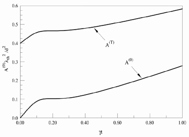
Figure 1: The functions $A^{(0)}(t)$ and $A^{(T)}(t)$ multiplied by $\lambda_{\mathrm{th}}^{2}/d^{2}$ plotted vs. $\gamma t$. The parameters chosen are $\lambda_{\mathrm{th}}=4\sigma$ and $kT=5\hbar\gamma$.

The first two terms in brackets in (27) correspond to a pair of Gaussian wave packets of the form (13), centered initially at $x_{0}=\pm d/2$ and propagating independently. We can call these the direct terms. The third term is an interference term. The direct terms are a maximum at their centers, which are drifting toward the origin but for $d\gg\sigma$ will for short times be well away from the origin. The interference term is a maximum at the origin and initially its peak height is exactly twice that of either of the direct terms. (However, as one can readily verify, the area under the interference term is independent of time and a factor $e^{-d^{2}/8\sigma^{2}}$ smaller than the area under the direct terms.) The factor $e^{-A^{(0)}(t)}$, equal to the ratio of the peak height of the interference term to twice the peak height of the either of the direct terms, is taken as a measure of the interference in phase space. In Fig. 1 we show $A^{(0)}$ as a function of $\gamma t$ and there we see that for $\gamma t\ll 1$, $A^{(0)}$ is linear in $t$. Using the expressions (11) for the quantities $A_{11}^{(0)}$ and (5) for $G$ we can readily show that for short times

$$A^{(0)}(t)\cong\frac{d^{2}}{\lambda_{\mathrm{th}}^{2}}\gamma t,$$ (29)

where $\lambda_{\mathrm{th}}$ is the mean de Broglie wavelength,

$$\lambda_{\mathrm{th}}=\frac{\hbar}{\sqrt{mkT}}.$$ (30)

For a separation large compared with the thermal de Broglie wave length, this corresponds to a decay of the peak height of the interference term on a time scale short compared with $\gamma^{-1}$,

$$\tau_{d}=\frac{\lambda_{\mathrm{th}}^{2}}{d^{2}}\gamma^{-1}.$$ (31)

This is the frequently appearing ”decoherence time” [7].

It is of interest to form the probability distribution, which in general is given by

$$P(x;t) = \int_{-\infty}^{\infty}dpW(q,p;t)$$ (32)

$$= \frac{1}{2\pi\hbar}\int_{-\infty}^{\infty}dPe^{ixP/\hbar}\tilde{W}(0,P;t).$$

Using the expression (26) for the Wigner characteristic function, this can be written

$$P(x;t) = \frac{1}{2(1+e^{-d^{2}/8\sigma^{2}})}[P^{(0)}(x-m\dot{G}\frac{d}{2})+P^{(0)}(x+m\dot{G}\frac{d}{2})$$ (33)

$$+2a(t)\exp\{-\frac{m^{2}\dot{G}^{2}d^{2}}{8A_{11}^{(0)}}\}P^{(0)}(x)\cos\frac{\hbar Gdx}{4\sigma^{2}A_{11}^{(0)}}),$$

where

$$P^{(0)}(x)=\frac{1}{\sqrt{2\pi A_{11}^{(0)}}}\exp\{-\frac{x^{2}}{2A_{11}^{(0)}}\}$$ (34)

is the probability distribution for a single minimum uncertainty wave packet initially centered a the origin and we have introduced the attenuation coefficient,

$$a(t)=\exp\{-\frac{\left\langle X^{2}\right\rangle d^{2}}{8\sigma^{2}A_{11}^{(0)}}\}.$$ (35)

The attenuation coefficient is a measure of the interference as it would be observed in the probability distribution. We should emphasize that the probability distribution can be directly measured. This is to be contrasted with the Wigner distribution in phase space, which is not directly observable.

The integrated probability in the interference term is equal to $e^{-d^{2}/8\sigma^{2}}$, independent of time. For $d\gg\sigma$ this is negligibly small. But it is the amplitude of the interference fringes that is observed and measured by the attenuation coefficient (35).

For short times, $\gamma t\ll 1$, using the expressions (6) for $\left\langle X^{2}\right\rangle$ and (11) for $A_{11}^{(0)}$, we see that the attenuation coefficient takes the form

$$a(t)\cong\exp\{-\frac{t^{3}}{3\tau_{d}[t^{2}+(2m\sigma^{2}/\hbar)^{2}]}\}.$$ (36)

This initially falls very slowly from unity, but after a time $2m\sigma^{2}/\hbar$ (the time for the mean square width $\Delta x^{2}$ to double) will decay with a characteristic time $3\tau_{d}$, where $\tau_{d}$ is the characteristic time (31) for the decay of the interference term in the Wigner function.

With no coupling to the bath the interference pattern in the probability distribution would not appear until the direct terms begin to overlap due to wave packet spreading. Taking $\gamma\rightarrow 0$ in the expression (11) for the mean square width, we see that this would be a time of order $t_{\mathrm{mix}}=2m\sigma d/\hbar\ll\tau_{d}$. What this means is that neither the rapid disappearance of the interference term in the Wigner distribution, nor the corresponding rapid decay of the attenuation coefficient, can could be directly observed. All that can be seen is the non-appearance of the interference term in the probability distribution.

4.2 Initial particle temperature equal to that of the bath

The corresponding results for the particle initially at the temperature $T$ of the bath are obtained using the prescription (19). The result is

$$W(q,p;t) = \frac{1}{2(1+e^{-d^{2}/8\sigma^{2}})}\left\{W^{(T)}(q-\frac{m\dot{G}d}{2},p-\frac{m^{2}\ddot{G}d}{2})\right.$$ (37)

$$+W^{(T)}(q+\frac{m\dot{G}d}{2},p+\frac{m^{2}\ddot{G}d}{2})$$

$$\left.+2e^{-A^{(T)}(t)}W^{(T)}(q,p)\cos\Phi^{(T)}(q,p:t)\right\},$$

where

$$A^{(T)}(t) = \frac{(A_{11}^{(T)}-\frac{\hbar^{2}G^{2}}{4\sigma^{2}})(A_{22}^{(T)}-\frac{\hbar^{2}m^{2}\dot{G}^{2}}{4\sigma^{2}})-(A_{12}^{(T)}-\frac{\hbar^{2}mG\dot{G}}{4\sigma^{2}})^{2}}{A_{11}^{(T)}A_{22}^{(T)}-A_{12}^{(T)2}}\frac{d^{2}}{8\sigma^{2}}$$

$$\Phi^{(T)}(q,p;t) = \frac{(GA_{22}^{(T)}-m\dot{G}A_{12}^{(T)})q+(m\dot{G}A_{11}^{(T)}-GA_{12}^{(T)})p}{A_{11}^{(T)}A_{22}^{(T)}-A_{12}^{(T)2}}\frac{\hbar d}{4\sigma^{2}}.$$ (38)

This expression for the Wigner function has the same form as that found above for the case where the initial particle temperature is zero. The only difference is that $A_{jk}^{(0)}\rightarrow A_{jk}^{(T)}$. The area under the interference term is still independent of time and smaller than the area under the direct terms by the same factor $e^{-d^{2}/8\sigma^{2}}$. The main difference is that the peak height of the interference term is much reduced. The ratio of the peak height of the interference term to twice that of the direct terms is given by the factor $e^{-A^{(T)}(t)}$ but, as we see in Fig. 1, $A^{(T)}$ no longer vanishes at $t=0$. Instead, we now find for $\gamma t\ll 1$,

$$A^{(T)}(t)\cong\frac{d^{2}}{2\lambda_{\mathrm{th}}^{2}+8\sigma^{2}}.$$ (39)

For separation large compared with both the thermal de Broglie wavelength and the slit width, this will be a large number and the peak height of the interference term will be correspondingly small. Thus, we see that there is no time scale for the disappearance of the interference term, it is already negligibly small at $t=0$. We might say that this is just the point. What has occurred is that an incoherent superposition of pure states has wiped out the interference term. In the present case this is the result of the initial preparation of the state. In the previous case of an initial pure state, this occurs as a result of the ”warming up” of the particle in a time $\tau_{d}$. In either case the interference term is gone long before its effect could be observed in the probability distribution.

The probability distribution is of the same form (33), but with $A_{11}^{(T)}(t)$ replacing $A_{11}^{(0)}(t)$. The attenuation coefficient is now given by

$$a(t)=\exp\{-\frac{(\left\langle X^{2}\right\rangle+mkTG^{2})d^{2}}{8\sigma^{2}A_{11}^{(T)}}\}$$ (40)

For $\gamma t\ll 1$ this becomes

$$a(t)\cong\exp\{-\frac{kTd^{2}}{8m\sigma^{4}}t^{2}\}$$ (41)

These results for short times are identical with those obtained from an exact calculation assuming entanglement of the particle with the bath at all times [7]). Since the coupling to the bath, as measured by the decay rate $\gamma$, does not appear they can also be obtained from a calculation without dissipation using only the familiar formulas of elementary quantum mechanics [10]. Thus we see that, while the exact master equation gives here correct results, it does so only for times so short that coupling to the bath can be neglected.

5 Density matrix

The density matrix is a Hermitian operator, $\rho$, defined such that for any wave function $\psi$ corresponding to a state of the particle in the Hilbert space $\left\langle\psi,\rho\psi\right\rangle$ is the probability that the system is in the state. From the notion of probability, we see immediately the the density matrix must be a positive definite operator. Consider the eigenfunctions $\phi_{a}$ and the corresponding eigenvalues $p_{a}$ of the density matrix,

$$\rho\phi_{a}=p_{a}\phi_{a}.$$ (42)

Clearly, the eigenvalue $p_{a}$ is the probability that the system is in state $\phi_{a}$ and is therefore necessarily positive. We assume the density matrix is normalized, so that

$$\sum_{a}p_{a}=1.$$ (43)

This is a sum of positive terms equal to unity. It follows immediately that

$$\mathrm{Tr}\{\rho^{2}\}=\sum_{a}p_{a}^{2}\leq 1.$$ (44)

Moreover, the equality holds if and only if there is exactly one eigenstate with probability one, all others having probability zero. This is exactly the condition (9) for a pure state.

In coordinate space the elements of the density matrix are given in terms of the Wigner characteristic function by the formula:

$$\left\langle x\left|\rho\right|x^{\prime}\right\rangle = \int_{-\infty}^{\infty}dpe^{i(x-x^{\prime})p/\hbar}W(\frac{x+x^{\prime}}{2},p)$$ (45)

$$\frac{1}{2\pi\hbar}\int_{-\infty}^{\infty}dPe^{i(x+x^{\prime})P/2\hbar}\tilde{W}(x^{\prime}-x,P).$$

The normalization condition (43) becomes

$$\mathrm{Tr}\{\rho\}=\int_{-\infty}^{\infty}dx\left\langle x\left|\rho\right|x\right\rangle=\tilde{W}(0,0)=1.$$ (46)

That is, the Wigner characteristic function corresponding to a normalized density matrix must have the value unity at the origin.

Next consider

$$\mathrm{Tr}\{\rho^{2}\} = \int_{-\infty}^{\infty}dx\int_{-\infty}^{\infty}dx^{\prime}\left\langle x\left|\rho\right|x^{\prime}\right\rangle\left\langle x^{\prime}\left|\rho\right|x\right\rangle$$ (47)

$$= \frac{1}{2\pi\hbar}\int_{-\infty}^{\infty}dQ\int_{-\infty}^{\infty}dP\left|\tilde{W}(Q,P)\right|^{2},$$

where we have used that fact that $\tilde{W}(-Q,-P)=\tilde{W}(Q,P)^{\ast}$. Thus, the condition (44) takes the form

$$\frac{1}{2\pi\hbar}\int_{-\infty}^{\infty}dQ\int_{-\infty}^{\infty}dP\left|\tilde{W}(Q,P)\right|^{2}\leq 1,$$ (48)

with the equality holding if and only if the density matrix is that of a pure state. This is the condition (9) for a pure state.

5.1 Gaussian wave packet

Consider now the case of an initial state corresponding to a single minimum uncertainty wave packet, for which the Wigner characteristic function at time $t$ is given in Eq. (10). The evaluation of the formula (45) for the matrix element of the density operator involves a single Gaussian integral. The result can be written

$$\left\langle x\left|\rho(t)\right|x^{\prime}\right\rangle=\exp\{i\frac{m^{2}\ddot{G}}{\hbar}x_{0}(x-x^{\prime})\}R(x-m\dot{G}x_{0},x^{\prime}-m\dot{G}x_{0};t),$$ (49)

where we have introduced

$$R(x,x^{\prime};t)=\frac{1}{\sqrt{2\pi A_{11}^{(0)}}}\exp\{-\frac{\frac{4}{\hbar^{2}}(A_{11}^{(0)}A_{22}^{(0)}-A_{12}^{(0)2})(x-x^{\prime})^{2}+(x+x^{\prime})^{2}}{8A_{11}^{(0)}}+i\hbar\frac{A_{12}^{(0)}(x^{2}-x^{\prime 2})}{2\hbar^{2}A_{11}^{(0)}}\},$$ (50)

which is the matrix element corresponding to a single wave packet initially centered at the origin. Using the expressions (5) for the Green function and (11) for $A_{jk}^{(0)}(t)$, we see that viewed in the $xx^{\prime}$ plane the absolute value of the density matrix, $\left|\left\langle x\left|\rho(t)\right|x^{\prime}\right\rangle\right|$, consists of a single Gaussian peak. This peak is initially centered at $x=x^{\prime}=x_{0}$ and circularly symmetric with width $\sigma$. In the course of time the center of the peak drifts to the origin while stretching in the direction $x=x^{\prime}$.

For short times, the density matrix is not necessarily positive. The simplest way to see this is to form $\mathrm{Tr}\{\rho^{2}\}$, using the above expression for the density matrix element or evaluating directly the expression (47). In either case we find

$$\mathrm{Tr}\{\rho^{2}\}=\frac{\hbar}{2\sqrt{A_{11}^{(0)}A_{22}^{(0)}-A_{12}^{(0)2}}}.$$ (51)

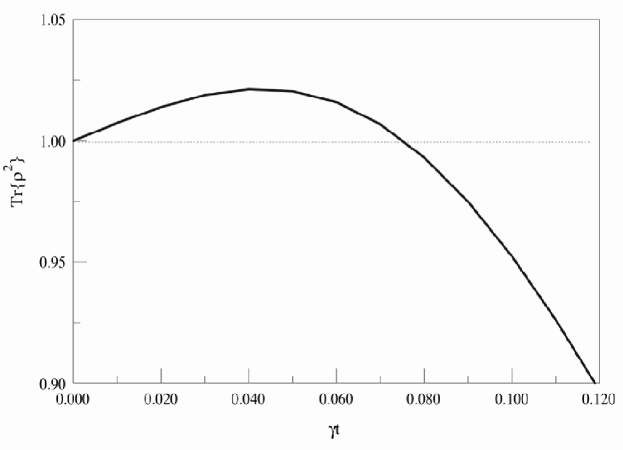
Figure 2: $\mathrm{Tr}\{\rho^{2}\}$ for an initial minimum uncertainty wave packet. The parameters chosen are $\lambda_{\mathrm{th}}=4\sigma,kT=5\hbar\gamma$, the same as for Fig. 1. Note that at short times $\mathrm{Tr}\{\rho^{2}\}>1.$

In Fig. 2 we show a plot over a short initial time interval of this result, evaluated using the expressions (11) for the $A_{jk}^{(0)}$ with parameters $\lambda_{\mathrm{th}}=4\sigma$, $kT=5\hbar\gamma$. There we see clearly that the condition (44) is violated for short times. It follows that for such times there must be negative eigenvalues; the density matrix is not positive-definite. We gain some insight into this phenomenon if we use the expressions (11) to expand

$$\mathrm{Tr}\{\rho^{2}\}\cong 1+(1-4\frac{\sigma^{2}}{\lambda_{\mathrm{th}}^{2}})\gamma t+\cdots.$$ (52)

From this we see that $\mathrm{Tr}\{\rho^{2}\}$ will increase above unity whenever $\lambda_{\mathrm{th}}>2\sigma$. The failure of positivity occurs for a sharply peaked wave packet.

To see explicitly this failure of positivity, it will be sufficient to take $x_{0}=0$. We then form the expectation of the density matrix with a wave function $\psi(x)\propto d\phi(x,0^{+})/dx$, where $\phi(x,0^{+})$ is the state immediately after the coupling to the bath (given in Eq. (18) with $x_{0}=0$). Explicitly,

$$\psi(x)=\frac{x}{\sigma(2\pi\sigma^{2})^{1/4}}\exp\{-(\frac{1}{4\sigma^{2}}+i\frac{m\gamma}{2\hbar})x^{2}\}.$$ (53)

With this,

$$\left\langle\psi,\rho(t)\psi\right\rangle = \int_{-\infty}^{\infty}dx\int_{-\infty}^{\infty}dx^{\prime}\psi^{\ast}(x)\left\langle x\left|\rho(t)\right|x^{\prime}\right\rangle\psi(x^{\prime})$$ (54)

$$= \frac{-2[1-\frac{4}{\hbar^{2}}(A_{11}^{(0)}A_{22}^{(0)}-A_{12}^{(0)2})]}{[(1+\frac{A_{11}}{\sigma^{2}})(1+\frac{4\sigma^{2}(A_{11}^{(0)}A_{22}^{(0)}-A_{12}^{(0)2})}{A_{11}})+\frac{4\sigma^{2}(A_{12}^{(0)}+m\gamma A_{11}^{(0)})^{2}}{\hbar^{2}A_{11}}]^{3/2}}.$$

This expectation will be negative whenever $4(A_{11}^{(0)}A_{22}^{(0)}-A_{12}^{(0)2})/\hbar^{2}<1$, that is exactly for those times when $\mathrm{Tr}\{\rho^{2}\}$ given by (51) is greater than one.

We have seen that general solution of the exact master equation results in a density matrix that can have negative eigenvalues. How can it be that an exact result can lead to such an unphysical consequence? The answer, of course, is that we been able to give a non-trivial meaning to the solution only in the high temperature limit, which involves a serious approximation (neglect of zero-point oscillations). It is this approximate result that fails the positivity test.

5.2 Wave packet pair

For the wave packet pair the Wigner characteristic function at time $t$ is given by (26). With this the formula (45) for the matrix element of the density operator becomes a standard Gaussian integral. The result is

$$\left\langle x\left|\rho(t)\right|x^{\prime}\right\rangle = \frac{1}{2(1+e^{-d^{2}/8\sigma^{2}})}$$ (55)

$$\times[\exp\{iL\frac{d}{2}(x-x^{\prime})\}R(x-m\dot{G}\frac{d}{2},x^{\prime}-m\dot{G}\frac{d}{2})$$

$$\exp\{-iL\frac{d}{2}(x-x^{\prime})\}R(x+\frac{m\dot{G}d}{2},x^{\prime}+\frac{m\dot{G}d}{2})$$

$$+e^{-A^{(0)}}\exp\{iM\frac{d}{2}(x+x^{\prime})\}R(x-K\frac{d}{2},x^{\prime}+K\frac{d}{2})$$

$$+e^{-A^{(0)}}\exp\{-iM\frac{d}{2}(x+x^{\prime})\}R(x+K\frac{d}{2},x^{\prime}-K\frac{d}{2})],$$

where $R(x,x^{\prime};t)$ is is the matrix element (50) corresponding to a single wave packet initially centered at the origin and to shorten the expressions we have introduced

$$K=\frac{\hbar^{2}(m\dot{G}A_{11}^{(0)}-GA_{12}^{(0)})}{4\sigma^{2}(A_{11}^{(0)}A_{22}^{(0)}-A_{12}^{(0)2})},\quad L=\frac{m^{2}\ddot{G}}{\hbar}.,\quad M=\frac{\hbar(m\dot{G}A_{12}^{(0)}-GA_{22}^{(0)})}{4\sigma^{2}(A_{11}^{(0)}A_{22}^{(0)}-A_{12}^{(0)2})}.$$ (56)

Viewed in the $xx^{\prime}$ plane, the density matrix element (55) will shows four peaks exactly of the form (49) of single wave packets; two diagonal peaks centered at $x=x^{\prime}=\pm m\dot{G}d/2$  and two off-diagonal peaks centered at $x=-x^{\prime}=\pm Kd/2$. The off-diagonal peaks are multiplied by the same factor $e^{-A^{(0)}(t)}$ that multiplies the interference term in the Wigner function (37). The result is that under the condition $d\gg\lambda_{\mathrm{th}}$, while the peaks slowly broaden and drift toward the origin, the off diagonal peaks rapidly shrink in amplitude. Thus, the two descriptions of the disappearance of the interference term, that in terms of the Wigner function and that in terms of the density matrix element, are entirely equivalent. In this connection note that the diagonal density matrix element is the probability distribution (33). The description in terms of the Wigner function has the advantage of being real, so somewhat simpler. Neither the Wigner distribution in phase space nor the density matrix element in $xx^{\prime}$ space is directly observable, so either description is theoretical.

6 Conclusion

We have exhibited a number of significant failures of the exact master equation: Due to the irreparable divergence the solution strictly does not exist except in the high temperature limit. Even in that approximation the solution breaks translational invariance. Finally, the solution corresponds to a density matrix that can have negative expected values. But we must remember that the derivation of the equation as well as its solution are formally correct. Rather, the failures can all be traced back to the assumption of an unentangeled initial state. The picture of a particle suddenly clamped to a bath corresponds to no physically realizable operation. Even when the initial particle temperature is adjusted to that of the bath it receives a violent squeeze toward the origin. From this follows the ”unphysical” consequences: correctly described by the exact master equation. Unfortunately, the final assessment is that the exact master equation is of  very limited utility.

In fact, in an exact description the particle must be coupled to the bath (entangled) at all times. Think of the example of the blackbody radiation field, which is coupled to the particle through its charge that can in no way be switched on or off. In physical applications the coupling to the radiation field is sufficiently weak that a description in terms of the familiar weak coupling master equation (of Lindblad form) is appropriate, but the effects of renormalization and zero-point oscillations are nevertheless present at all times.

References

• [1] G. W. Ford and R. F. O’Connell, Phys. Rev. D 64 105020 (2001).
• [2] G. W. Ford and M. Kac, J. Stat. Phys. 45, 803 (1987).
• [3] L. van Hove, Physica 18, 145 (1952).
• [4] H. Araki and S. Yamagami, Publ. Res. Inst. Math. Sci. 18, 283 (1982).
• [5] G. V. Efimov and W. von Waldenfels, Annals of Physics 233, 182 (1994).
• [6] G. Lindblad, Commun. Math. Phys. 48, 119 (1976).
• [7] G. W. Ford J. T. Lewis and R. F. O’Connell, Phys. Rev. A 64, 032101 (2001).
• [8] G. A. Garrrett, A. G. Rojo, A. K. Sood, J. F. Whittaker and R. Merlin, Science 275, 1638 (1997).
• [9] G. W. Ford and R. F. O’Connell, American Journal of Physics 70, 319 (2002).
• [10] M. Murakami, G. W. Ford and R. F. O’Connell, Laser Physics 13, 180 (2003).
Refer to caption