Quantum heat engine with multi-level quantum systems

Abstract

By reformulating the first law of thermodynamics in the fashion of quantum-mechanical operators on the parameter manifold, we propose a universal class of quantum heat engines (QHE) using the multi-level quantum system as the working substance. We obtain a general expression of work for the thermodynamic cycle with two thermodynamic adiabatic processes, which are implied in quantum adiabatic processes. We also classify the conditions for a 3-level QHE to extract positive work, which is proved to be looser than that for a 2-level system under certain conditions. As a realistic illustration, a 3-level atom system with dark state configuration manipulated by a classical radiation field is used to demonstrate our central idea.

I Introduction

A usual heat engine operates between two heat baths, the temperature difference between which completely determines the maximum efficiency of the heat engine. Correspondingly, it is inferred that no power can be extracted if the two baths have the same temperature. But things become different when we use quantum matter as the working substance. Quantum effects can highlight the thermodynamic differences between classical and quantum working substance of a heat engine. Recently, great efforts book has been devoted to the investigation of the quantum effect of the working substance. Some exotic phenomena were discovered, most of which concerns the following three aspects: The first aspect is whether we can improve the efficiency of the QHE to a level beyond the classical limit. For example, M. O. Scully et al. Scully-science ; Scully-book ; Zubairy-book proposed a quantum-electrodynamic heat engine that can exceed the maximum limit by using the photon gas as working substance. The second aspect is how we can better the work extraction during a Carnot cycle. T. D. Kieu present a new type of QHE Kieu-PRL ; Kieu1 , in which the contact time is precisely controlled (without reaching thermal equilibrium) and the two heat baths are specifically modified. This QHE can extract more work than the other model in thermal equilibrium case. The third aspect is about the constraints of the temperatures of the two heat baths, under which positive work can be extracted. It is clear that a classical heat engine can extract positive work when and only when $T_{h}>T_{l}$. Here, $T_{h}$ and $T_{l}$ are the temperatures of the source and the sink. But for a QHE, some exotic phenomena may occur. One example is given in Ref. Scully-science , in which positive work can be extracted even from a single heat bath, i.e., $T_{h}=T_{l}$; Another example is the simplest 2-level QHE model in Refs. Kosloff1 ; Kieu1 , in which positive work can be extracted only when $T_{h}$ is greater than $T_{l}$ to a certain extent.

We consider the third aspect in detail. In Refs. Kosloff1 ; Kieu1 , the QHE works between the source and sink at temperatures $T_{h}$ and $T_{l}$ respectively. Within a cycle, the level spacing $\Delta$ changes between $\Delta^{h}$ and $\Delta^{l}$. For such a QHE, the system couples to the bath for a sufficiently long time until they reach the thermal equilibrium state. Then positive work can be performed when and only when $T_{h}>T_{l}(\Delta^{h}/\Delta^{l})$ (condition $I$). This result implies a broad validity of the second law and shows by how much $T_{h}$ should be greater than $T_{l}$ such that the positive work can be extracted. This constraints about temperatures is obviously counter-intuitively different from that of a classical heat engine. Now we wonder whether it is a universal condition for all multi-level QHE. Actually T. D. Kieu has considered two special cases, the simple harmonic oscillator and the infinite square well, in (the appendices of) Ref. Kieu1 . As to the two special cases, because all the level spacings change in the same ratio, the PWC has the same form as that for a 2-level case Infinite well . In this article, we will prove that the PWC for a 3-level QHE can be looser compared to a 2-level case under our criterion when the level spacings change properly in the thermodynamic cycle.

This paper is organized as follows: In section $II$, we formulate a quantum version of the first law of thermodynamics for a multi-level quantum system. In section $III$, we discuss the relationship between the quantum adiabatic process and the thermodynamic adiabatic process. In section $IV$ we analyze the quantum thermodynamic cycle of a universal QHE. The obtained results are more universal than those obtained from the 2-level system Arnaud ; He ; Kosloff2 . In section $V$, we classify the 3-level QHE according to the changes of level spacings. We find under certain condition the PWC for a 3-level QHE can be looser than its counterpart for a 2-level case. A realistic model—a 3-level atomic system with dark state structure manipulated by a classical radiation field—is given to demonstrate our central idea in section $VI$.

II Quantum Version of the First Law of thermodynamics

We consider the QHE with a $N$-level system as its working substance. The system eigenenergies vary adiabatically with the parameters $\mathbf{R=(}R_{1,}R_{2,}...,R_{M,}\mathbf{)}$ in an $M$-dimensional manifold $\mathbf{M}$. One can manipulate the parameters to implement the quantum adiabatic process, which does not excite the transitions among the instantaneous eigenstates $|n\rangle\equiv$ $|n[\mathbf{R}]\rangle$ of the Hamiltonian $\widehat{H}=\widehat{H}[\mathbf{R}]$ with the instantaneous eigenvalues $E_{n}$ $\equiv$ $\left|E_{n}[\mathbf{R}]\right\rangle$. Usually the density operator $\widehat{\rho}$ is a function of both the external parameters $\mathbf{R}$ and the thermodynamic parameter, i.e., the temperature $T$. So we need to extend the manifold $\mathbf{M}$ to include $T$. For example, the heat transfer can be also caused by the change of the temperature. In this sense, we define the differential one-form on the ($M+1)$-dimensional “manifold” $\mathbf{MT}$: $\mathbf{\{X=(R,}T\mathbf{)\}}$ by $dF=\nabla_{R}Fd\mathbf{R+}d_{T}F$ for any function $F$. We emphasize that $d_{T}$ may be a discrete variation $\delta_{T}$ in the time domain. Then in this sense $\mathbf{MT}$ is no longer a generic manifold.

During a thermodynamic cycle, work is done by or on the system when the mechanical parameters $R$ vary slowly. While heat is transferred when the quantum state or density operator changes as the temperature varies discretely. At two different instants $t=$ $0$ and $\tau_{2},$ the system contacts with the source and sink at temperature $T_{h}$ and $T_{l}$ respectively to reach thermodynamic equilibrium. The couplings of the system to such different heat baths yield the discrete change of the probabilities distribution in every eigenstate. We consider the infinitesimal variation

$$dU=Tr(\widehat{\rho}d_{\mathbf{R}}\widehat{H})+Tr(\widehat{H}d\widehat{\rho})$$ (1)

of the expectation value $U=Tr(\widehat{\rho}\widehat{H})$ of the Hamiltonian, where we have introduced the density operator of the state $\widehat{\rho}$. $dU$ contains two parts corresponding to the changes of the Hamiltonian and the density operator respectively. Here, the operator 1-form, on the sub-manifold $\mathbf{M}$, can be written as

$$d_{\mathbf{R}}\widehat{H}=d_{\mathbf{R}}\widehat{Q}+d_{\mathbf{R}}\widehat{W},$$ (2)

which is the infinitesimal variation of $\widehat{H}$. Here, the off-diagonal part

$$d_{\mathbf{R}}\widehat{Q} = \sum_{m\neq n}\langle m|d_{\mathbf{R}}\widehat{H}|n\rangle|m\rangle\langle n|$$

$$= \sum_{n}E_{n}d_{\mathbf{R}}(|n\rangle\langle n|)$$

is the heat operator and the diagonal part

$$d_{\mathbf{R}}\widehat{W} = \sum_{m}\langle m|d_{\mathbf{R}}\widehat{H}|m\rangle|m\rangle\langle m|$$

$$= \sum_{m}(d_{\mathbf{R}}E_{m})|m\rangle\langle m|$$

is the work operator. To derive the above equations we have used the Feynman-Hellman theorem $\langle m|d\widehat{H}|m\rangle=dE_{m}$ and the formula $\langle m|d\widehat{H}|n\rangle=$ $(E_{n}-E_{m})\langle m|d|n\rangle.$

Upon a first glance, the above definitions of the work operator $d_{\mathbf{R}}\widehat{W}$ and the heat operator $d_{\mathbf{R}}\widehat{Q}$ are reasonable. Intuitively speaking, the work can be done only when the $R$-dependent eigenenergy of inner states change. This process is just described by $d_{\mathbf{R}}\widehat{W}$. The off-diagonal elements of the infinitesimal variation of $\widehat{H}$ indicates the transitions among the inner energy levels and thus results in the heat transfer. The term $d_{\mathbf{R}}(|n\rangle\langle n|)$ interprets the heat transferred to or from a quantum system along with the change of the projections to the instantaneous eigenstate. Physically it means the changing of the occupation probabilities rather than the $\mathbf{R}$-dependent eigenvalues themselves. In addition, when the quantum state $\widehat{\rho}$ itself changes due to the varying of both the control parameters $\mathbf{R}$ and the thermodynamic parameter $T$, the heat is also transfered. This kind of heat tansfer is described by the second term on the left hand side of the Eq. (1).

In comparison with the existing studies about QHE Kieu1 , we write down the infinitesimal energy $dU=$ ${\mathchar 22\relax\mkern-11.0mud}Q+{\mathchar 22\relax\mkern-11.0mud}W$, where the infinitesimal heat transferred ${\mathchar 22\relax\mkern-11.0mud}Q$ and work done ${\mathchar 22\relax\mkern-11.0mud}W$ are identified respectively as two path dependent differentials

$${\mathchar 22\relax\mkern-11.0mud}Q = Tr(\widehat{H}d\widehat{\rho})+Tr(\widehat{\rho}d_{\mathbf{R}}\widehat{Q})=\sum_{m}E_{m}\,dp_{m},$$ (5)

$${\mathchar 22\relax\mkern-11.0mud}W = Tr(\widehat{\rho}d_{\mathbf{R}}\widehat{W})=\sum_{m}p_{m}\,dE_{m}.$$ (6)

Here $p_{m}=\langle m|\widehat{\rho}|m\rangle$ are the corresponding occupation probabilities in the instantaneous states $|m\rangle$.

We would like to emphasize that the above two equations were even obtained in many previous references Kieu1 ; He ; Kosloff3 . But here we present a general derivation, the process of which shows the differences between work and heat in the view of quantum mechanics. Substantially, we give the microscopic definitions of work and heat based on the non-adiabatic transitions among the instantaneous eigenstates of the time-dependent Hamiltonian.

III From quantum adiabatic evolution to thermodynamic adiabatic process

The term “adiabatic process” is usually used in both quantum mechanics and thermodynamics, and seemingly has different meanings for these two cases. Actually, a quantum adiabatic process implies a thermodynamic adiabatic process. But not all thermodynamic adiabatic processes is caused by quantum adiabatic processes Kieu1 ; yukawa . This understanding is crucial for the following analysis about the thermodynamic cycle of the QHE.

In quantum mechanics, the adiabatic process is described by the time evolution of a quantum system with slowly changing parameters. When these parameters vary slow enough, the transitions among the instantaneous eigenstates $|n[\mathbf{R}]\rangle\equiv$ $|n(t)\rangle$ are forbidden, i.e., the system will keep in the $n$-th instantaneous eigenstate $|n(t)\rangle$ if the system is initially in the eigenstate $|n(0)\rangle$ at time $t=0$. Generally speaking, starting with the initial state $|\psi(0)\rangle=\sum\limits_{n}c_{n}|n(0)\rangle$, the system will evolve into

$$|\psi(t)\rangle=\sum\limits_{n}c_{n}\exp[-i\int_{0}^{t}E_{n}(t^{\prime})dt+i\gamma_{n}]|n(t)\rangle,$$ (7)

where

$$\gamma_{n}=\int_{0}^{t}\left\langle n(t^{\prime})\right|\frac{d}{dt^{\prime}}\left|n(t^{\prime})\right\rangle dt^{\prime}$$

is the so-called Berry’s phase. This conclusion implies that the occupation probability $\left|\left\langle n(t)\right.\left|\psi(t)\right\rangle\right|^{2}$ in an instantaneous eigenstate $|n(t)\rangle$ is adiabatically invariant. This result is also valid for the initial mixed state, e.g., the thermal equilibrium state

$$\widehat{\rho}(0)=\sum_{n}\rho_{nn}|n(0)\rangle\langle n(0)|,$$ (8)

where $\rho_{nn}$ are Gibbs probability distributions.

We illustrate a quantum adiabatic process and its corresponding thermodynamic adiabatic process in Fig. 1. An amount of ideal gas is constrained in a cylinder. The piston moves so slow that the gas is always kept in thermal equilibrium state. Usually no heat is gained or lost in a thermodynamic adiabatic process. Thus any isotropic process implies its adiabatic property. But all adiabatic process are not isentropic. For example, an adiabatic-free expansion is not isentropic. Now we prove a quantum adiabatic process illustrated in Fig. 1b microscopically leads to an isentropic process and thus a thermodynamic adiabatic process.

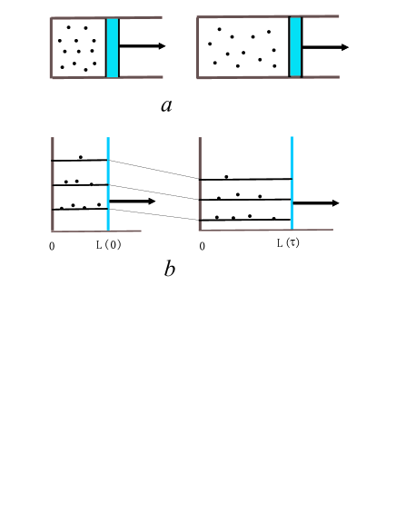
Figure 1: (color on line) Illustration of classical adiabatic process ($a$) and its quantum-mechanical counterpart ($b$). At time $t=0$, the piston (wall) locates at $L(0)$, and after a long time $t=\tau$, the piston (wall) moves slowly to $L(\tau)$. No change happens in the energy level populations during the adiabatic process.

In quantum mechanics, we describe the motion of these structureless gas atoms or molecules with an infinite potential well with one moving boundary (Fig. 1b). The piston or boundary moves so slow that the quantum adiabatic condition are satisfied adiabatic condition . Now we consider the microscopic definition of the thermodynamic entropy

$$S=-kTr\left(\widehat{\rho}[\mathbf{R}]\ln\widehat{\rho}[\mathbf{R}]\right).$$ (9)

The variation of the entropy due to the changes of the mechanical parameters $\mathbf{R}$ can be calculated as

$$d_{\mathbf{R}}S[\mathbf{R}]=-k\sum\limits_{n}\left(\rho_{nn}\ln\rho_{nn}+1\right)d_{\mathbf{R}}\rho_{nn}.$$ (10)

According to the quantum adiabatic theorem, the particle distributions in the instantaneous energy levesls are invariant during a quantum adiabatic process. Then, from Eq. (10), the entropy keeps unchanged. Therefore, it is concluded that the quantum adiabatic process of the microscopic particles just results in the thermodynamic adiabatic process of the macroscopic system.

The above arguments shows that the quantum adiabatic process in quantum mechanics can result in a thermodynamic adiabatic process. But we have to point out that not all thermodynamic adiabatic process are caused by the quantum mechanical adiabatic process. For example, in the thermodynamic adiabatic process of Fig. 1$a$ a single molecule may experience nonadiabatic transitions due to its interaction with other molecules.

IV Positive work done by multilevel QHE in a thermodynamic cycle

 Like the classical heat engine, a universal QHE also bases on a thermodynamic cycle. Mathematically, it can be understood as a close path $l$: $\{\mathbf{X}=(\mathbf{R},T)|\mathbf{X(0)=X(\tau}_{4}\mathbf{)}\}$ on the ($M+1)$-dimensional “manifold” $\mathbf{MT.}$ The efficiency of a universal QHE is $\eta_{q}=\Delta W/Q$  corresponding to the ratio of the work done to the heat absorbed during a cycle,

$$\Delta W = \oint{\mathchar 22\relax\mkern-11.0mud}W$$ (11)

$$Q = \int_{\mathbf{0}}^{\tau_{1}}{\mathchar 22\relax\mkern-11.0mud}Q,$$ (12)

where $\tau_{1}$ is the ending point of Step 1. A typical four-stroke QHE, consists of two quantum adiabatic and two isothermal processes, is a quantum analogue of the classical Otto engine, as illustrated in Fig. 2:

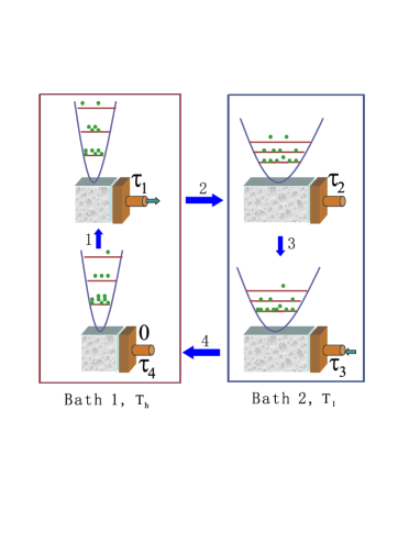
Figure 2: (color on line) The graphic sketch of a universal QHE model. From time $t=0$ to t=$\tau_{1}$, the system absorbs heat from the source (bath 1). From time $t=\tau_{1}$ to t=$\tau_{2}$, work is done by the system when the piston is pushed by the working substance. Step 3 (from time $t=\tau_{2}$ to t=$\tau_{3}$) and step 4(from time $t=\tau_{3}$ to t=$\tau_{4}$) are reversed processes of step 1 and step 2 with modification.

Steps 1 and Step 3 are two isothermal processes. During Step 1, i.e., from time $t=0$ to $t=\tau_{1}$, the system couples to the source (bath 1) at temperature $T_{h}$ and the level spacings keep unchanged. After absorbing energy from the heat source, the system reaches thermodynamic equilibrium state, which can be described by the density operator $\widehat{\rho}(\tau_{1})$. The heat absorbed during Step 1 is

$$Q=\int_{\mathbf{0}}^{\tau_{1}}\sum_{m}E_{m}\langle m|\delta_{T}\widehat{\rho}|m\rangle.$$ (13)

Step 3 is almost an inverse process of Step 1. From time $\tau_{2}$ to $\tau_{3}$, the system is brought to couple to the sink at temperature $T_{l}$. The density matrix changes into $\widehat{\rho}(\tau_{3})$ after releasing energy into the bath. In the above operations, the absorption and the release of energy during Steps 1 and Step 3 happen in quantum ways. Namely, they can only happen probabilistically. The corresponding probability depends on the details of the interactions and some intrinsic properties, e.g., the temperatures of the heat baths.

Steps 2 and Step 4 are two adiabatic processes. During Steps 2 the QHE performs positive work when the energy spacings decrease. Meanwhile the parameters $\mathbf{R}$ adiabatically change from $\mathbf{R}(\tau_{1})=\mathbf{R}(0)$ to $\mathbf{R}(\tau_{2})$. But the atomic probability distribution remains unchanged in this process. Step 4 is almost an inverse process of step 2, during which the system is removed from the sink and its energy gaps increase as an amount of work is done on the system. The net work done by the system during a cycle is

$$\Delta W=\left(\int_{\tau_{1}}^{\tau_{2}}+\int_{\tau_{3}}^{\tau_{4}}\right)\sum_{m}p_{m}dE_{m}.$$ (14)

The above results can give the known results in Kieu1 ; He ; Kosloff3 for a 2-level system.

We assume the thermal equilibrium Gibbs distributions for the heat bath. The system will eventually reach Gibbs distribtution

$$\widehat{\rho}(\tau)=Z^{-1}e^{-\beta_{s}\widehat{H}}=\sum_{m}p_{m}^{s}|m\rangle\langle m|$$ (15)

after coupling to the heat bath for a time much longer than the relaxation time $\gamma^{-1}$ of the considered system. The occupation probability in the instantaneous eigenstate $|m\rangle$ is

$$p_{m}^{s}(t)=\frac{e^{-\beta_{s}E_{m}(T_{s})}}{Z^{s}},$$ (16)

which depends on the spectral structure and the temperature $T_{s}(s=h,l)$ of the relevant heat baths. Here $\beta_{s}=1/(KT_{s})$, and $K$ is the Boltzmann constant.  The partition function is defined by

$$Z^{s}=\sum_{m}e^{-\beta_{s}E_{m}(T_{s})}.$$ (17)

For the cyclic nature of QHE, the energy level spacings return at different instants. Then the net work done during a cycle can be calculated as

$$\Delta W=\sum_{m}\left[p_{m}^{h}(\tau_{1})-p_{m}^{l}(\tau_{3})\right]\Delta E_{m},$$ (18)

where

$$\Delta E_{m}=E_{m}(T_{h})-E_{m}(T_{l}).$$ (19)

Therefore, the PWC can be explicitly expressed as

$$\Delta W=\sum_{m}\left[p_{m}^{h}(\tau_{1})-p_{m}^{l}(\tau_{3})\right]\Delta E_{m}>0.$$ (20)

V Classification of positive work cycles for 3-level QHE

It is also known from Refs. Kieu1 ; Kosloff3 that the PWC for the 2-level QHE working between the source and sink at temperature $T_{h}$ and $T_{l}$ can be written as

$$T_{h}>T_{l}\frac{\Delta^{h}}{\Delta^{l}}.$$ (21)

Only when this PWC is satisfied can the positive work be extracted. This condition is counter-intuitively different from that $T_{h}>T_{l}$ for a classical heat engine. Now, we naturally ask a question: Is this condition (21) universal for a multi-level QHE? In this section we will prove that, if the energy levels change properly, the PWC for a 3-level system can be looser than that for a 2-level system (21).

Our model considered here is a 3-level system with the adjustable level spacings $\Delta_{1}^{s}$ and $\Delta_{2}^{s}$ $(s=h,l)$, as illustrated in Fig. 3. Here, we denote the ground state, the first excited state and the second excited state with subscripts $0$, $1$ and $2$ respectively. We also introduce the dependent parameters $\Delta^{s}=\Delta_{1}^{s}+\Delta_{2}^{s},(s=h,l)$. For this kind of 3-level systems, if the PWC (20) can be reduced to

$$\left\{\begin{array}[]{c}T_{h}>T_{l}\left(\Delta^{h}/\Delta^{l}\right)\theta\\ T_{h}>T_{l}\left(\Delta_{1}^{h}/\Delta_{1}^{l}\right)\theta^{\prime}\end{array}\right.,$$ (22)

meanwhile both $\Delta^{l}/\Delta^{h}<\theta<1$ and $\Delta_{1}^{l}/\Delta_{1}^{h}<\theta^{\prime}<1$ are satisfied, then we say the PWC is looser than that for a 2-level case since the PWCs for both the two substructures are looser than that for a 2-level system (21). The two substructures are formed by combining level $0$ with level $1$ and level $2$ respectively. We will prove in the following there indeed exist such cases for a 3-level system. This means that the PWC for a 3-level system can be improved in comparison with that for a 2-level case when the levels change properly.

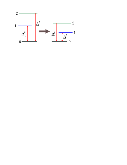
Figure 3: (color on line) A sketch of an adiabatic evolution of the level spacings of a 3-level system during the step 2. $\Delta_{i}^{h}$ and $\Delta_{i}^{l}(i=1,2)$ are the two level spacings when coupling to the source and the sink. $\Delta^{h}(\Delta^{l})$ is the maximum level spacing, i.e., $\Delta^{s}=\Delta_{1}^{s}+\Delta_{2}^{s},(s=h,l)$.

For the 3-level case we rewrite the expression (18) of $\Delta W$ in a more explicit form

$$\Delta W=\frac{G(\Delta,\Delta_{1})+G(\Delta_{1},\Delta)}{Z^{h}(T_{h})Z^{l}(T_{l})},$$ (23)

where $Z_{s}(T_{s})$ is the partition function for the three level case.

$$G(\Delta,\Delta_{1}) = \Theta(\Delta,\Delta_{1})(\Delta^{h}-\Delta^{l}),$$ (24)

$$\Theta(\Delta,\Delta_{1}) = e^{-\beta_{h}\Delta^{h}}-e^{-\beta_{l}\Delta^{l}}$$

$$+e^{-\beta_{h}\Delta^{h}-\beta_{l}\Delta_{1}^{l}}-e^{-\beta_{h}\Delta_{1}^{h}-\beta_{l}\Delta^{l}}.$$

Obviously $\Delta W$ is completely determined by $T_{s},$ $\Delta_{1}^{s}$ and $\Delta_{2}^{s}(s=h,l)$, which is independent of the details of the changing of the level spacings. Thus, we only care about the initial level spacing $\Delta_{i}^{h}$ and the final level spacing $\Delta_{i}^{l}$ in considering the thermodynamic cycle.

However, at arbitrary finite temperature, the PWC (20) is too complicated to be understood directly, so we switch to considering its high temperature limit. In this limit the PWC (20) can be simplified as

$$L\left[F(\xi,\eta)-\frac{T_{l}}{T_{h}}\frac{\Delta^{h}}{\Delta^{l}}F(\xi,\lambda)\right]\left(\Delta_{1}^{h}-\Delta_{1}^{l}\right)>0,$$ (26)

where we have introduced

$$F(\xi,\eta) = \left[\left(2\xi-1\right)+\left(2-\xi\right)\eta\right],$$

$$L = \frac{\Delta^{l}}{kT_{l}Z^{h}(T_{h})Z^{l}(T_{l})}$$ (27)

in terms of an independent set of parameters

$$\xi \equiv 1+\frac{\Delta_{2}^{h}-\Delta_{2}^{l}}{\Delta_{1}^{h}-\Delta_{1}^{l}};$$ (28)

$$\text{ }\eta \equiv \frac{\Delta_{1}^{l}}{\Delta^{l}};\text{ }\lambda\equiv\frac{\Delta_{1}^{h}}{\Delta^{h}}.$$

According to the requirement of the quantum adiabatic evolution, the level spacings $\Delta_{1}^{s}$ and $\Delta_{2}^{s}$ are always kept positive during the two quantum adiabatic process. Therefore, the parameters $\eta$ and $\lambda$ range in the interval $(0,1)$, i.e., $0<\eta,$ $\lambda<1$.

In principle, we can classify the multi-level QHE according to the changes of the level spacings in the thermodynamic cycles. As to the 3-level QHE, there are altogether four sorts of operations corresponding to the following four cases:

$$\left\{\begin{array}[]{c}(I).\Delta_{1}^{h}-\Delta_{1}^{l}>0,\text{ }\Delta_{2}^{h}-\Delta_{2}^{l}>0\\ (II).\Delta_{1}^{h}-\Delta_{1}^{l}>0,\text{ }\Delta_{2}^{h}-\Delta_{2}^{l}<0\\ (III).\Delta_{1}^{h}-\Delta_{1}^{l}<0,\text{ }\Delta_{2}^{h}-\Delta_{2}^{l}>0\\ (IV).\Delta_{1}^{h}-\Delta_{1}^{l}<0,\text{ }\Delta_{2}^{h}-\Delta_{2}^{l}<0\end{array}\right.,$$ (29)

as schematized in Fig. 4.

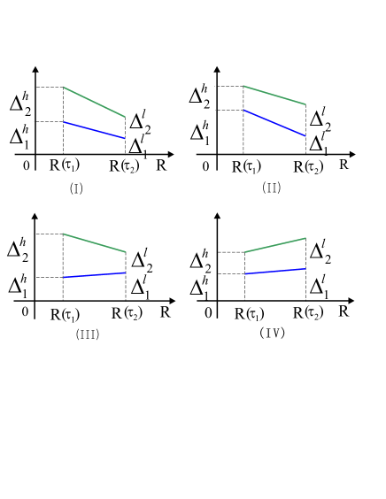
Figure 4: (color online) Sketch map of four sorts of 3-level QHE. There are altogether four kinds of 3-level QHE, as illustrated above, according to the changes of the level spacings during step 2. Here (I), (II), (III) and (IV) are corresponding to case (I) to case (IV) in Eq. (29) respectively.

Before analyzing the four cases in detail, we intuitively consider the physical mechanism that a 3-level QHE may better the work done. Namely, the PWC can be relaxed compared to that for a 2-level case. For instance, if the lower level spacing does not change during step 2 (see Fig. 5 $a$), $\Delta_{1}^{h}=\Delta_{1}^{l}$ (dashed line), the 3-level QHE reduced to a 2-level case, then the PWC cannot be bettered. However, when it comes to $\Delta_{1}^{h}>\Delta_{1}^{l}$ (solid line), the lowing of energy level $1$ produces extra work to better the PWC. On the contrary, if the level spacings changes as that in Fig. 5 $b$, $\Delta_{1}^{h}<\Delta_{1}^{l}$ ( solid line), the raising of the energy level $1$ makes the PWC become worse. These two cases are corresponding to Case (I) and Case (III) in Fig. 4. We expect that the 3-level QHE of Case (I) can better the work extraction but Case (III) can not. We will try to prove this result and determine the physical parameters that can better the work extraction in the following detailed analysis. Firstly we consider Case (I).

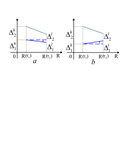
Figure 5: (color online) A 3-level QHE built up by adding a third level to the 2-level QHE. Intuitively speaking, it can make the PWC looser (better the work extraction) when the new level helps to produce positive work ($a$), but makes the PWC worse when it cost energy ($b$).

Case (I): Physically, $\Delta_{1}^{h}-\Delta_{1}^{l}>0$ and $\Delta_{2}^{h}-\Delta_{2}^{l}>0$ mean both of the two level spacings decrease adiabatically during step 2. Since $\Delta_{1}^{h}-\Delta_{1}^{l}>0$, the PWC (26) can be simplified as

$$F(\xi,\eta)T_{h}>T_{l}F(\xi,\lambda)\frac{\Delta^{h}}{\Delta^{l}}.$$ (30)

By noticing that $\xi>1$, $F(\xi,\eta)>1$ and $F(\xi,\lambda)>1$ in Case (I), the above PWC (30) can be further simplified as

$$T_{h}>T_{l}\frac{\Delta^{h}}{\Delta^{l}}\theta.$$ (31)

Here, the dimensionless parameter $\theta$ is defined by

$$\theta=\frac{F(\xi,\lambda)}{F(\xi,\eta)}.$$ (32)

Aiming to construct a 3-level QHE with a relaxed constraints (22) on temperatures, we need to analyze in what conditions $\theta<1$ is satisfied. Obviously, as to $\theta<1$, i.e., $\left(2-\xi\right)\lambda<\left(2-\xi\right)\eta$, there are two solutions. Solution $I$:

$$\xi>2\ and\ \lambda>\eta,$$ (33)

and Solution $II$:

$$1<\xi<2\ and\ \lambda<\eta.$$ (34)

For simplicity, we define a set of independent physical parameters in terms of the ratios of three level spacings to $\Delta_{1}^{h}$,

$$r_{1}^{l}=\frac{\Delta_{1}^{l}}{\Delta_{1}^{h}},r_{2}^{l}=\frac{\Delta_{2}^{l}}{\Delta_{1}^{h}},r_{2}^{h}=\frac{\Delta_{2}^{h}}{\Delta_{1}^{h}}.$$ (35)

Then it is easy to see that

$$r_{1}^{l}<1,r_{2}^{h}>r_{2}^{l}$$ (36)

are implied in our presupposition of Case (I).

Based on the above analysis, Solution $I$ can be explicitly obtained to be

$$\left\{\begin{array}[]{c}r_{2}^{h}+r_{1}^{l}-r_{2}^{l}>1\\ r_{2}^{l}>r_{1}^{l}r_{2}^{h}\end{array}\right..$$ (37)

We combine Eqs. (36) and (37) and plot them in a 3-dimensional figure in coordinates of $r_{1}^{l}$, $r_{2}^{l}$ and $r_{2}^{h}$. The solution is a 3-dimensional domain enveloped by a curved surface, $r_{2}^{l}=r_{1}^{l}r_{2}^{h}$ (denoted by $A$) and two planes $r_{2}^{h}=1-r_{1}^{l}+r_{2}^{l}$ (denoted by $B$) and $r_{1}^{l}=0$. Any representative point in this domain can determine a 3-level QHE, which can extract positive work under the conditions $T_{h}>T_{l}\left(\Delta^{h}/\Delta^{l}\right)\theta$ and $\Delta^{l}/\Delta^{h}<\theta<1$.

We further consider whether Solution $I$ is consistent with the second inequality of Eq. (22). Fortunately we can easily find such $\theta^{\prime}$ smaller than unity for $\Delta_{1}^{h}/\Delta_{1}^{l}>\Delta^{h}/\Delta^{l}$ in Solution $I$. Thus, according to the the definition (22), it is proved that the PWC for 3-level system can be looser than that for a 2-level case if the level spacings change properly.

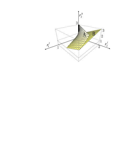
Figure 6: (color online) Diagram of solution I of case I. For a given $\Delta_{1}^{h}$, when $\Delta_{1}^{l},\Delta_{2}^{l}$ and $\Delta_{2}^{h}$ are properly chosen such that the point $(r_{1}^{l},r_{2}^{l},r_{2}^{h})$ is in the enveloped range, positive work can be extracted under a looser condition.

Similarly we rewrite Solution $II$ (34) in terms of $r_{1}^{l}$, $r_{2}^{l}$ and $r_{2}^{h}$,

$$\left\{\begin{array}[]{c}r_{2}^{h}+r_{1}^{l}-r_{2}^{l}<1\\ r_{2}^{l}<r_{1}^{l}r_{2}^{h}\end{array}\right..$$ (38)

Together with (36), we illustrate the result in Fig. 7. The physical meaning is the same as that of Solution $I$. But Solution $II$ is not an ideal solution like Solution $I$, for we cannot find such solution that satisfy the second inequality.

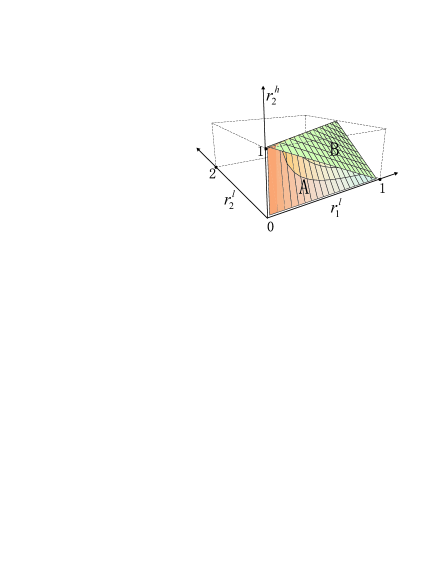
Figure 7: (color online) Diagram of solution II of case I. The representative points in the enclosed range are the results of inequalities(38), and the physical meaning is similar to that of Fig. 6.

In order to make our result clear, we illustrate the above results in comparison with that for a classical heat engine and a 2-level QHE in Fig. 8 and Fig. 9. As to a classical heat engine, e.g., a Carnot engine, the PWC is $T_{h}>T_{l}$, and the net work $\Delta W$ is a linear function of $T_{h}$ for a given $T_{l}$. But for a 2-level QHE, the PWC is Eq. (21), and the net work is not a linear function of $T_{h}$, as illustrated in Fig. 8.

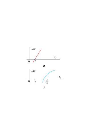
Figure 8: (color online) Sketch map of the net work $\Delta W$ as a function of $T_{h}$ for a given $T_{l}$. Part $a$ illustrates a classical Carnot engine, while part $b$ illustrates a 2-level QHE.

As to Solution $I$ of case $I$ of the 3-level QHE, the PWC is looser than that for a 2-level case, because the PWC for both the two substructures are looser than that for the 2-level system, as illustrated in Fig. 9$a$. However, as to Solution $II$, the PWC is not looser than that for a 2-level case, for the PWC for one substructure is looser than that for the 2-level system, but the other is not, as illustrated in Fig. 9$b$.

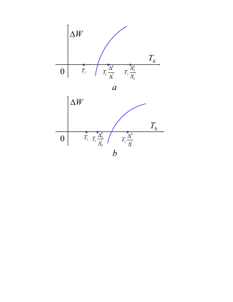
Figure 9: (color on line) Similar to Fig. 8. Part $a$ illustrates Solution $I$ of Case $I$ of the 3-level QHE, and Part $b$ illustrates Solution $II$ of Case $I$ of the 3-level QHE.

Case (II): In this case $\Delta_{1}^{h}-\Delta_{1}^{l}>0$ and $\Delta_{2}^{h}-\Delta_{2}^{l}<0.$ Physically, this means that the upper level spacing increases while the lower level spacing decreases during step 2. We will prove in the following in this case there exist no such solution about $\Delta_{i}^{h}$ and $\Delta_{i}^{l}$ that can better the work extraction compared to a 2-level case.

To prove this conclusion we need to distinguish the following 4 situations:

$$\mathbf{a} : F(\xi,\eta)>0,F(\xi,\lambda)>0,$$ (39)

$$\mathbf{b} : F(\xi,\eta)>0,F(\xi,\lambda)<0,$$

$$\mathbf{c} : F(\xi,\eta)<0,F(\xi,\lambda)<0,$$

$$\mathbf{d} : F(\xi,\eta)<0,F(\xi,\lambda)>0.$$

a: The PWC (26) can  be reduced to Eq. (31). Similar to above analysis, if we want to find a looser PWC, $\theta$ should be smaller than unity, i.e.,$\ \theta<1$. By noticing $\xi<1$ in Case (II), $\theta<1$ can be further simplified as $\lambda<\eta$, i.e.,

$$\frac{\Delta_{1}^{l}}{\Delta_{1}^{h}}>\frac{\Delta_{2}^{l}}{\Delta_{2}^{h}}.$$ (40)

However, this inequality is incompatible with the two constraints of Case (II): $\Delta_{1}^{h}-\Delta_{1}^{l}>0$ and $\Delta_{2}^{h}-\Delta_{2}^{l}<0$. Thus, in this situation, the PWC is no looser than that for a 2-level QHE for $\theta>1$.

b: The two inequalities $F(\xi,\eta)>0$ and $F(\xi,\lambda)<0$ can be reduced to

$$\frac{1-2\eta}{2-\eta}<\xi<\frac{1-2\lambda}{2-\lambda}.$$ (41)

Thus we can obtain the inequality $\eta>\lambda$, i.e.,

$$\frac{\Delta_{1}^{l}}{\Delta_{1}^{h}}>\frac{\Delta_{2}^{l}}{\Delta_{2}^{h}}.$$

Similarly, this inequality is incompatible with $\Delta_{1}^{h}-\Delta_{1}^{l}>0$ and $\Delta_{2}^{h}-\Delta_{2}^{l}<0$. Thus, in Case (II) $F(\xi,\eta)>0$ and $F(\xi,\lambda)<0$ can not be satisfied simultaneously. Therefore, there does not exist the PWC looser than that for a 2-level QHE in this situation.

c: The PWC can now be reduced to be

$$T_{h}<T_{l}\frac{\Delta^{h}}{\Delta^{l}}\theta.$$ (42)

By noting that we have assumed beforehand $T_{h}>T_{l}$. Only when $(\Delta^{h}/\Delta^{l})\theta>1$, the QHE is probable to extract positive work. From Eq. (39), $F(\xi,\eta)<0$ is always satisfied in condition c. Then $(\Delta^{h}/\Delta^{l})\theta>1$ can be reduced to

$$\xi^{2}-\xi+1=(\xi-\frac{1}{2})^{2}+\frac{3}{4}<0.$$ (43)

Obviously this inequality has no solution to the real parameter $\xi$. Therefore the positive work can not be extracted in this situation.

d: The PWC can now be reduced to $T_{h}<T_{l}(\Delta^{h}/\Delta^{l})\theta.$ The left hand side in the inequality is positive while the right hand side is negative (for $\theta<0$). It is obvious that, there does not exist a PWC looser than that for a 2-level QHE in this situation, either.

In summary, we cannot find a PWC looser than that for a 2-level case in Case (II). After similar analysis about Case (III) and Case (IV), we find there is no desired solution in Case (III) and Case (IV) either. In conclusion, only in Case (I) can we find such desired solutions that the 3-level QHE can better the work extraction compared to the 2-level case. This conclusion agrees with the result obtained from our foregoing intuitional consideration.

We also would like to mention that under the criterion (22) we find the PWC for a 3-level QHE can be looser than that for a 2-level case. If we use other criterions, the result may be different. For example, if we use $\Delta_{2}$ instead of $\Delta$ in the first inequality of (22), we can not find such 3-level QHE that whose PWC is looser than that for a 2-level case. Actually, for Case (I), the PWC (22) can always be simplified to inequality (31) $T_{h}>T_{l}\left(\Delta^{h}/\Delta^{l}\right)\theta$. It can be proved that the coefficient $\left(\Delta^{h}/\Delta^{l}\right)\theta$ satisfies

$$\min\left\{\frac{\Delta_{1}^{h}}{\Delta_{1}^{l}},\frac{\Delta_{2}^{h}}{\Delta_{2}^{l}}\right\}\leqslant\frac{\Delta^{h}}{\Delta^{l}}\theta\leqslant\max\left\{\frac{\Delta_{1}^{h}}{\Delta_{1}^{l}},\frac{\Delta_{2}^{h}}{\Delta_{2}^{l}}\right\}.$$ (44)

This conclusion is also true for $n$-level QHE. Namely, if the PWC for a $n$-level QHE can be expressed as $T_{h}>T_{l}\kappa$, then it can be proved that the coefficient $\kappa$ satisfies

$$\min\left\{\frac{\Delta_{1}^{h}}{\Delta_{1}^{l}},\cdots,\frac{\Delta_{n}^{h}}{\Delta_{n}^{l}}\right\}\leqslant\kappa\leqslant\max\left\{\frac{\Delta_{1}^{h}}{\Delta_{1}^{l}},\cdots,\frac{\Delta_{n}^{h}}{\Delta_{n}^{l}}\right\}.$$ (45)

Here $\Delta_{i}^{h}$ and $\Delta_{i}^{l}$ are the energy gaps between the $i$th and the $\left(i-1\right)$th energy level in Steps 1 and Step 3. Specifically, when all the level spacings change in the same ratio, i.e., $\Delta_{1}^{h}/\Delta_{1}^{l}=\Delta_{2}^{h}/\Delta_{2}^{l}=\cdots=\Delta_{n}^{h}/\Delta_{n}^{l}$, no matter how the spectral structure is, the PWC for such a system has the same form as that for a 2-level case $T_{h}>T_{l}\left(\Delta^{h}/\Delta^{l}\right)$. The harmonic oscillator and the infinite well potential are two good examples Kieu1 ; Infinite well .

VI Illustration: 3-level atom with dark state

In the preceding section, we found in proper conditions the PWC for the 3-level QHE can be looser that that for a 2-level QHE (condition $I$). In this section, we will use a concrete example to demonstrate our results. We consider a toy model with 3-level system couples to a classical single-mode external field. The levels are adjusted by the external light field, which plays a similar role to an ideal piston in classical heat engine. In this ideal case we need not to consider the work for the controlling field to adjust the level during the adiabatic process. Just through this external field the work (either positive or negative) done on the 3-level system means the change of energy of the 3-level system. Namely, in our theoretical studies, no extra work is required for the controlling field since we regarded the field as a part of the external entries .

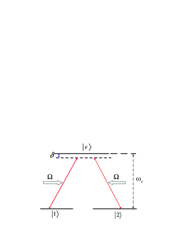
Figure 10: (color online) The sketch of a 3-level QHE model. A $\lambda$-type 3-level system interacting with a single classical radiation field. $\left|e\right\rangle$ is the exited state, while $\left|1\right\rangle$ and $\left|2\right\rangle$ are the two degenerate ground states.

The model Hamiltonian Scully2 reads

$$\widehat{H}=\hbar\delta\left|e\right\rangle\left\langle e\right|+\Omega\left(\left|e\right\rangle\left\langle 1\right|+\left|e\right\rangle\left\langle 2\right|+h.c\right),$$ (46)

where $\delta$ is the common detuning (see Fig. 10). We have set the eigenenergy of the two degenerate ground states $\left|1\right\rangle$ and $\left|2\right\rangle$ as zero, and that of the excited state $\left|e\right\rangle$ as $\hbar\omega_{e}$. $\Omega$ is the complex Rabi frequency associated with the coupling of the field mode of frequency $\omega$ to the atomic transition $\left|e\right\rangle\rightarrow\left|1\right\rangle$ ($\left|e\right\rangle\rightarrow\left|2\right\rangle$). The detuning of $\omega$ is $\delta$,

$$\omega=\omega_{e}-\delta.$$ (47)

We solve the eigen-equation, and obtain the eigenvalues

$$E_{0} = 0,$$ (48)

$$E_{+} = \frac{1}{2}\left(\hbar\delta+\sqrt{\left(\hbar\delta\right)^{2}+8\left|\Omega\right|^{2}}\right),$$

$$E_{-} = \frac{1}{2}\left(\hbar\delta-\sqrt{\left(\hbar\delta\right)^{2}+8\left|\Omega\right|^{2}}\right).$$

Then this QHE has two level spacings:

$$\Delta_{1} = E_{0}-E_{-}=\frac{1}{2}\left(\sqrt{\left(\hbar\delta\right)^{2}+8\left|\Omega\right|^{2}}-\hbar\delta\right),$$ (49)

$$\Delta_{2} = E_{+}-E_{0}=\frac{1}{2}\left(\sqrt{\left(\hbar\delta\right)^{2}+8\left|\Omega\right|^{2}}+\hbar\delta\right).$$

The two level spacings are functions of two independent parameters $\delta$ and $\left|\Omega\right|$. During Steps 2 the level spacings change adiabatically from $\Delta^{h}\left(\Delta_{1}^{h}\right)$ to $\Delta^{l}\left(\Delta_{1}^{l}\right)$ when the two parameters change slowly from ($\delta^{h}$, $\left|\Omega^{h}\right|$) to ($\delta^{l}$, $\left|\Omega^{l}\right|$). According to the systematical analysis in last section, this model can indeed serve as an improved 3-level QHE if the two parameters change properly. We plot the energy levels $\Delta\left(\delta\text{, }\left|\Omega\right|\right)$ and $\Delta_{1}\left(\delta\text{, }\left|\Omega\right|\right)$ in Fig. 11.

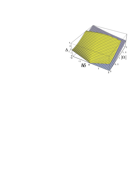
Figure 11: (color online) The two level spacings as functions of $\hbar\delta$ and $\left|\Omega\right|$. The upper curved surface represents $\Delta^{s}$ while the lower one represents $\Delta_{1}^{s}$.

In a thermodynamic cycle, the level spacing changes adiabatically between $\Delta_{i}^{h}$ and $\Delta_{i}^{l}$ during the two adiabatic processes. For convenience, we define

$$K^{s}=\sqrt{\left(\hbar\delta^{s}\right)^{2}+8\left|\Omega^{s}\right|^{2}}.$$ (50)

The two constraints of Case (I) in Eq. (29) can also be expressed in terms of $K^{s}$ and $\delta^{s}$:

$$\frac{K^{l}-\hbar\delta^{l}}{K^{h}-\hbar\delta^{h}}<1,\frac{K^{l}+\hbar\delta^{l}}{K^{h}+\hbar\delta^{h}}<1.$$ (51)

Substituting Eq. (49) into Eq. (37), we get the Solution $I$ in terms of $K^{s}$ and $\delta^{s}$,

$$\left\{\begin{array}[]{c}\delta^{l}K^{h}>\delta^{h}K^{l},\\ \delta^{h}>\delta^{l}.\end{array}\right.$$ (52)

Combine Eqs. (51) and (52), we find the inequalities hold only when $\delta^{h}>\delta^{l}>0$. Thus the solution (52) can be reduced into a more compact form

$$\left\{\begin{array}[]{c}\delta^{h}>\delta^{l}>0,\\ \left|\Omega^{l}/\delta^{l}\right|<\left|\Omega^{h}/\delta^{h}\right|.\end{array}\right.$$ (53)

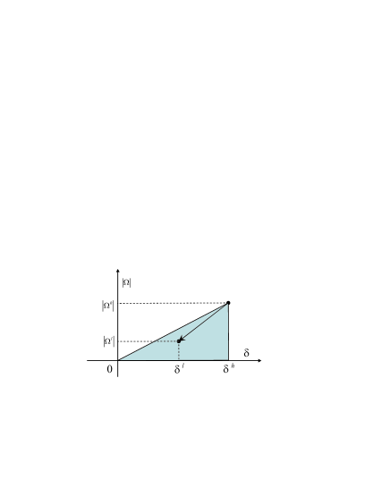
Figure 12: (color online) Illustration of Eq. (53). In this solution the QHE can extract positive work while the PWC is looser comparing with that for 2-level QHE.

During step 2 of a thermodynamic cycle, we assume the initial level spacings are $\Delta^{h}$ and $\Delta_{1}^{h}$ corresponding to two positive parameters $\delta^{h}$ and $\left|\Omega^{h}\right|$. Then the level spacings change adiabatically to $\Delta^{l}$ and $\Delta_{1}^{l}$ when the two parameters change slowly to ($\delta^{l}$, $\left|\Omega^{l}\right|$). The above result (53) shows that, only when the final point ($\delta^{l}$, $\left|\Omega^{l}\right|$) locates in the shaded triangle in Fig. 12 can we make the PWC looser compared to condition $I\$for a 2-level case.

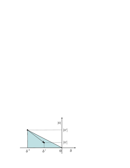
Figure 13: (color online) Illustration of Eq. (54). The physical meaning is similar to that of Fig. 12. But this is not an ideal solution.

Similarly, we substitute Eq. (49) into Eq. (38) and then obtain Solution $II$ in terms of $K^{s}$  and $\delta^{s}$.

$$\left\{\begin{array}[]{c}\delta^{h}<\delta^{l}<0,\\ \left|\Omega^{l}/\delta^{l}\right|<\left|\Omega^{h}/\delta^{h}\right|.\end{array}\right.$$ (54)

The physical meaning is almost the same as that of Fig. 12. For the initial parameters $\delta^{h}$ and $\left|\Omega^{h}\right|$, only when the final point ($\delta^{l}$, $\left|\Omega^{l}\right|$) locates in the shaded triangle in Fig. 13 can the first inequality of (22) be satisfied, but the second is still not. Thus Solution $II$ is not a desired solution.

Before concluding this section, we would like to address a crucial problems in the physical implementation of the above “dark state model”. It is obvious that we do work on the system when varying the parameters $\delta$ and $\left|\Omega\right|$ in step 4. But how is the work extracted out of the system can not be imagined directly. Here, what we discussed in this section is only a toy mode to illustrate the basic spirit of physics in the quantum thermodynamic cycles. The work done by the system in step 2 can be indirectly understood as the consequence of the decrease of the system energy, which can be explicitly calculated from our foregoing analysis (see Eq. (6)) in section II.

VII Conclusion and remarks

We have quantum-mechanically formulated the work done and the heat transferred in the thermodynamic processes in association with the microscopic quantum transitions. A class of QHE were universally proposed by using a multi-level quantum system as the working substance and by deriving the thermodynamic adiabatic process from the quantum adiabatic process. We classified a 3-level QHE based on the changes of the level spacings, and found when the parameters (and thus the level spacings) change properly, a 3-level QHE can better the work extraction compared to a 2-level case.

Before concluding this paper we would like to point out that the two-parameter QHE proposed in the last section is only a toy model and one can not over estimate it. We have to say that the Hamiltonian for such an atomic system in the laboratory frame of reference is time-dependent and changes fast. Therefore one can roughly regarded it as something relevant to the system energy. It is still an open question to find a multi-level system with level spacings changing independently in practice.

We also remark that the discussion about QHE is essentially semi-classical because we quantize neither the heat bath nor the controllable external fields. To build a totally-quantum theory for QHE, one need to use the generalized master equations with and without memories. There are some interesting results in Refs. Bender1 ; Bender2 . How to develop our present studies within this theoretical framework is to be considered in our forthcoming investigations.

Acknowledgement: This work is supported by the NSFC with grant Nos. 90203018, 10474104 and 10447133. It is also funded by the National Fundamental Research Program of China with Nos. 2001CB309310 and 2005CB724508. We thank T. D. Kieu for helpful discussion.

References

- (1) D. P. Sheehan (Ed), Quantum limits to the second law: first international Conference, (Melville, New York, 2002).
- (2) M. O. Scully, M. S. Zubairy, G. S. Agarwal, H. Walther, Science 299, 862 (2003).
- (3) M. O. Scully, Quantum limits to the second law: first international Conference, edited by D.P.Sheehan (2002).
- (4) M. S. Zubairy, Quantum limits to the second law: first international Conference, edited by D.P.Sheehan (2002).
- (5) T. D. Kieu, Phys. Rev. Lett. 93, 140403 (2004).
- (6) T. D. Kieu, arXiv:quantum-ph/0311157 v5 22 Aug 2005.
- (7) T. Feldmann and R. Kosloff, Phys. Rev. E 61, 4774 (2000).
- (8) Similar to the harmonic oscillator, it is easy to prove that the PWC for the infinite square well model is , where and are the widths of the well in two steps.
- (9) J. Arnaud, L. Chusseau, F. Philippe, arXiv:quantum-ph/0211072 v2 2 Jun 2003.
- (10) J. He, J. Chen, B. Hua, Phys. Rev. E 65, 036145 (2002).
- (11) R. Kosloff, T. Feldmann, Phys. Rev. E 65, 055102(R) (2002).
- (12) E. Geva and R. Kossloff, J. Chem. Phys. 96, 3054 (1992).
- (13) H. Yukawa (Ed), Quantum Mechanics Vol I, 2nd Ed, (in Japanese), (Yan-Bo Bookshop, Tokyo, 1978).
- (14) C. P. Sun, J. Phys. A 21, 1595 (1988), Phys. Rev. D 41, 1318 (1990).
- (15) L. I. Schiff, Quantum Mechanics, 3rd ed., (McGRAW-HILL, Inc., New York, 1968).
- (16) M. O. Scully and M. S. Zubairy, Quantum Optics (Cambridge University Press, 1997).
- (17) C. M. Bender, D. C. Brody, B. K. Meister, Proc. R. Soc. Lond. A 458,1519 (2002).
- (18) C. M. Bender, D. C. Brody, B. K. Meister, J. Phys. A 33, 4427 (2000).