Entanglement distribution by an arbitrarily inept delivery service

Abstract

We consider the scenario where a company $C$ manufactures in bulk pure entangled pairs of particles, each pair intended for a distinct pair of distant customers. Unfortunately, its delivery service is inept – the probability that any given customer pair receives its intended particles is $S\in(0,1)$, and the customers cannot detect whether an error has occurred. Remarkably, no matter how small $S$ is, it is still possible for $C$ to distribute entanglement by starting with non-maximally entangled pairs. We determine the maximum entanglement distributable for a given $S$, and also determine the ability of the parties to perform nonlocal tasks with the qubits they receive.

I Introduction

Entanglement is an important resource in developing new quantum technologies. It is essential for many quantum information processing (QIP) tasks such as quantum computation, quantum teleportation and super-dense coding Nielsen ; Preskill . At least for pure states and two parties, the mathematical characterization of entanglement is well established. However, it is only recently that researchers have begun to ask questions about constrained entanglement. That is, entanglement that seems to exist in a system according to our conventional description of its quantum states may not exist (or at least may be of a different nature) because of constraints that limit our ability to process the quantum information in the system. In the case that the constraint (either fundamental or practical) can be expressed as a super-selection rule (SSR), the modification to our notions of entanglement are now well studied VerCir03 ; WisVac03 ; BarWis03 ; BarDohSpeWis05 ; Schuch04 ; Kitaev04 .

In this paper we consider a different sort of constraint that can be understood from the following scenario. A company $C$ manufactures a pure entangled pair of particles for a pair of customers, and delivers one particle to each customer. For reasons of economy it manufactures these particle pairs in bulk, and delivers to a large number of customer pairs. Unfortunately, its delivery service is inept, meaning that the probability that any given customer pair receives particles that were manufactured as an entangled pair is $S\in(0,1)$. Moreover, the customers cannot detect whether an error has occurred. For example, the particles may be indistinguishable. Thus the constraint is caused by a loss of classical information, as in Ref. Eisert (the differences with their situation will be expanded upon later). We prove the surprising result that, no matter how small the success probability $S$, $C$ can still distribute entanglement. We also discuss how this scenario, although it might sound artificial, may actually be relevant to the production of entangled photon pairs.

This paper is organized as follows. In Sec. II we present the scenario in more detail. We then prove in Sec. III that entanglement distribution is always possible, and follow this up by determining the optimal entanglement distribution protocol in Sec IV. Since distillation may not always be practical, in Sec. V we study the ability of the mixed-up states to demonstrate nonlocality without distillation. Section VI concludes with a discussion of the practical implications of our theory in quantum optics and ensemble quantum information processing.

II Scenario

We can now be more detailed about the scenario outlined above. First, we assume that company $C$ manufactures pure, identical, entangled pairs of qubits. Ideally, it delivers one qubit from each pair to remote customers, say, $A_{1}$ in Albuquerque, $A_{2}$ in Ajax, $A_{3}$ in Athens etc., and the other qubit from each pair to their respective partners $B_{1}$ in Belfast, $B_{2}$ in Brisbane, $B_{3}$ in Berlin etc. This is illustrated in Fig. 1(a), and would allow any pair of customers, $A_{i}$ and $B_{i}$, to undertake nonlocal quantum information tasks such as teleportation Bennett93 or violating a Bell inequality Bell .

Now we will define the success probability $S$ of the service to be the probability that any pair $(A_{i},B_{i})$ receives their intended qubits in a pure entangled state. We will assume that $S$ is independent of $i$, and also that a failure (which occurs with probability $1-S$) means that one of $A_{i}$ and $B_{i}$ receive a qubit other than the one intended for them, so that the qubits are uncorrelated. For example, for three pairs of customers if $S=1/3$ then a typical outcome would be the case shown in Fig. 1(b), where only one successful delivery takes place.

In this case illustrated in Fig. 1(b), one pair of customers is still happy, as it knows it has received a pure entangled pair. But what if the customers know that the delivery service is inept, so that $S<1$, but have no way of knowing whether they actually received their intended qubits? This is illustrated by Fig. 1 (c), where the customers know that $S=1/3$ as in Fig. 1 (b), but now all are unsure as to whether they have an entangled pair.

Note that we need not assume that the qubits intended for the customers $\{A_{i}\}$ are mixed up only amongst themselves; they could be mixed up with the qubits for the $\{B_{i}\}$. However, for simplicity, let us make that assumption. If, for the moment, we further assume that the delivery service is otherwise completely inept, so that for $N$ pairs of customers $S=1/N$, then our scenario is close to that considered by Eisert et al. Eisert (which was formalized as a $S_{N}$-SSR in Ref. BarWis03 ). The key difference is that (in our language) Eisert et al. allow for all $N$ of the $A_{i}$s to get together to do joint operations on their qubits, and likewise the $B_{i}$s. In our scenario this is inappropriate as the customers are distant from, and unaware of, each other. Thus, except between members of a pair, even classical communication is forbidden.

The above considerations establish that in our scenario, each pair of customers can be treated independently of each other pair. Thus, to determine whether any entanglement has been delivered to a particular pair of customers, whom we will call $A$ and $B$, we consider their state of knowledge. Say the pure entangled states prepared by $C$ are represented by $\rho_{AB}$. Then $A$ and $B$ know that they received this state with probability $S$ and that they received uncorrelated qubits (derived by throwing away their entangled partner) with probability $1-S$. Thus, their state of knowledge is

$${\cal M}[\rho_{AB}]\equiv S\rho_{AB}+(1-S){\rm Tr_{B}}[\rho_{AB}]\otimes{\rm Tr_{A}}[\rho_{AB}].$$ (1)

Here ${\cal M}$ is a nonlinear map that describes the mixing-up caused by the inept delivery service. Nonlinear maps of this sort, with $S=0$, have been studied before as a “universal disentanglement machine” Terno . For a single system (as opposed to an ensemble of identical systems) this map is unphysical Terno ; physical universal disentanglers which operate imperfectly or probabilistically have also been considered Buzek .

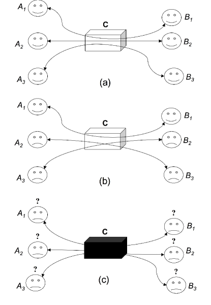
Figure 1: In (a) we have an ideal case where $S=1$ and all the customers receive their intended qubits. Situation (b) would be typical if $S=1/3$, only one pair out of three receives their intended qubits. In reality (c) would occur, the customers know that $S<1$ and are unsure as to whether they have received an entangled pair.

Naïvely, we might expect that under almost complete mixing-up (that is, $S\ll 1$) the customers would lose their entanglement. After all, how could two parties have nonlocal correlations if their subsystems almost certainly never interacted with each other in the past? Surprisingly, this is not the case, as we now show.

III Entanglement Distribution is Always Possible

To carry out many QIP tasks it is useful to work with maximally entangled states such as Bell pairs. However, Bell pairs have actually been found to be the most fragile states under the influence of certain types of noise Fragilityexamples . This suggests that Bell states may be fragile under the influence of mixing-up as we have defined it. Therefore, to distribute entanglement when mixing up will occur, it may be more useful to prepare entangled states of the form $\rho_{AB}=|{\psi_{a}}\rangle\langle{\psi_{a}}|$, where

$$|{\psi_{a}}\rangle=a|{0,0}\rangle+\sqrt{1-a^{2}}|{1,1}\rangle,$$ (2)

with $a\in[0,1]$. If $a=1/\sqrt{2}$ then $|{\psi}\rangle$ is a maximally entangled Bell state. If $a=0$ or $1$ then $|{\psi}\rangle$ is unentangled. Note that this state is symmetric under interchange of $A$ and $B$, so here we can allow for the delivery service to mix up qubits intended for the customers $\{A_{i}\}$ with those intended for the customers $\{B_{i}\}$.

To gain an insight into which states will be most robust we calculate the fidelity Jozsa , $f$, of the state under ${\cal M}$:

$$f=\langle{\psi_{a}}|{\cal M}\bigl{[}|{\psi_{a}}\rangle\langle{\psi_{a}}|\bigr{]}|{\psi_{a}}\rangle=1-3a^{2}(1-S)(1-a^{2}).$$ (3)

The minimum of Eq. (3) is at $a=1/\sqrt{2}$, so Bell states are also the most fragile states under the influence of mixing-up. By contrast, the fidelity of non-maximally entangled states with $a\ll 1$ remains high even when a large amount of mixing-up occurs (i.e. $S\ll 1$). This suggests that such states may be best for distributing entanglement under the map ${\cal M}$.

To determine this, we calculate the concurrence $\mathcal{C}$ Wootters98 of ${\cal M}[|{\psi_{a}}\rangle\langle{\psi_{a}}|]$:

$$\mathcal{C}=2Sa\sqrt{1-a^{2}}-2(1-S)a^{2}(1-a^{2}).$$ (4)

When $\mathcal{C}>0$ we know that entanglement has survived despite the mixing-up of the qubits. In particular, $\mathcal{C}>0$ iff (if and only if)

$$S>\frac{a(1-a^{2})}{\sqrt{1-a^{2}}+a-a^{2}}.$$ (5)

It is easy to verify that for any $S$, there is a range of $a$ values that satisfy this inequality. For $S\ll 1$, Eq. (5) is satisfied if $a<S$, as can be seen from the bottom left-hand corner of Fig. 2. Thus, entanglement can always be distributed by $C$ by preparing an initial state $|{\psi_{a}}\rangle$ with sufficiently little entanglement (the concurrence of $|{\psi_{a}}\rangle$ scales as $2a$ for $a\ll 1$). By contrast, ${\cal C}=0$ for Bell pairs when $S<1/3$, due to their fragility.

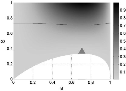
Figure 2: Diagram to illustrate conditions under which $C$ can distribute ‘useful’ entanglement. The colorbar gives an indication of the amount of entanglement at each point on the graph. The white region is defined by Eq. (5) and demonstrates where no entanglement is distributed. Above the dark line Eq. (8) is satisfied. Thus above this line undistilled pairs can be used to violate the CHSH-Bell inequality. In the gray regions below this line, entangled pairs are distributed. However it is unclear if these undistilled pairs may be used for nonlocal tasks. In the region marked by a gray triangle a LHVT for non-sequential POVM measurements exist (this coloring is separate from the gray scale).

IV Optimal Entanglement Distribution

We have shown that although inept delivery reduces the amount of entanglement that can be accessed, entanglement can still be distributed for arbitrarily low success probabilities. However, if this entanglement is to be used as a resource for QIP we need to know exactly how much entanglement can be accessed. In the regime $S\ll 1$, Eq. (4) becomes

$$\mathcal{C}\approx 2aS-2a^{2}.$$ (6)

The entanglement of formation $E_{F}$ Bennett96 for a pair of qubits is a monotonic function of the concurrence, as shown by Wootters Wootters98 . Thus the maximum of $\mathcal{C}$ corresponds to the maximum of $E_{F}$. It is clear from Eq. (6) that $\mathcal{C}$ (and thus $E_{F}$) is maximized for $a=S/2$. Thus, in the $S\ll 1$ regime we have an approximate analytical expression for the maximum amount of entanglement that can be distributed

$$E_{F}^{\rm max}\approx\frac{S^{4}}{4}\left[\log_{2}\left(\frac{1}{S}\right)+1+\frac{1}{4\ln(2)}\right].$$ (7)

A comparison of Eq. (7) and results for the maximum entanglement of formation which can be distributed (determined numerically) is shown in Fig. 3. Thus we can say that, given a success probability $S$, to distill a single Bell pair requires delivery of at least of order $4/S^{4}\log_{2}{S^{-1}}$ non-maximally entangled pairs.

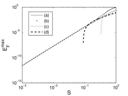
Figure 3: Diagram of entanglement distributed for given success probabilities. Curve (a) shows the maximum entanglement distributed. The curve (b) is an approximate expression for the maximum entanglement for $S$ given by Eq. (7). The plots (c) and (d) show the entanglement for the specific cases when $C$ distributes initial states (2) defined by $a=1/\sqrt{2}$ and $a=0.1$ respectively.

V Nonlocality Without Distillation

In some instances it may be impractical to perform distillation protocols to retrieve Bell pairs. Another interesting question is therefore whether or not the entanglement present in the initial pairs without distillation could be useful for some nonlocal task. One test of this is to see if a Bell inequality violation can be demonstrated.

While entanglement can be distributed for arbitrarily low $S$, this entanglement cannot be used to violate a Bell inequality at low $S$. For example, it is simple to show that the Clauser-Horne-Shimony-Holt (CHSH) Bell inequality CHSH is violated iff

$$S>\frac{1}{4(4a^{4}-4a^{2}-1)(4a^{4}-4a^{2}+1-\sqrt{4a^{4}-4a^{2}+3})}.$$ (8)

For Bell states this requires that $S>1/\sqrt{2}$, and for $a\neq 1/\sqrt{2}$ the requirement is more strict, as shown by the line in Fig. 2. It can thus be seen that relatively high success probabilities are required in order for the undistilled pairs to violate the CHSH inequality .

In the gray region of Fig. 2 below this line it is unclear whether or not the pairs can be used for nonlocal tasks without distillation. It may be possible to find other Bell inequalities which would allow a wider class of the undistilled pairs to be used to demonstrate nonlocality. However, we have shown that for at least part of this region there exists a local-hidden-variable theory (LHVT) for any non-sequential POV measurement Werner89 ; Barrett02 . That is, each party can make an arbitrary measurement, but is not allowed to communicate the result to the other party. The proof is straightforward and follows work of Barrett Barrett02 . He showed a LHVT exists under these conditions for the non-separable state (a Werner state)

$$\rho_{\rm B}=\frac{5}{12}|{\psi}\rangle\langle{\psi}|+\frac{7}{12}\left(\frac{I}{2}\otimes\frac{I}{2}\right),$$ (9)

where $|{\psi}\rangle$ is a Bell state ($a=1/\sqrt{2}$), and $I$ is the $2\times 2$ identity matrix.

We show that for some values of $a$, ${\cal M}\left[|{\psi_{a}}\rangle\langle{\psi_{a}}|\right]$ can be written as a convex combination of Eq. (9) and a separable state:

$$\rho={\cal M}\left[|{\psi}\rangle\langle{\psi}|\right]=c\rho_{\rm B}+(1-c)\rho_{\rm SEP},$$ (10)

where $0<c<1$. For such states $\rho$ it is clear that a LHVT exists, since such a theory always exists for separable states. By rearranging Eq. (10), we have

$$\rho_{\rm SEP}=(\rho-\rho_{\rm B})/(1-c).$$ (11)

Thus, in order for our LHVT to work, $\rho_{\rm SEP}$ should be a valid separable density matrix. For simplicity, we considered only $\rho_{\rm SEP}$ states that were diagonal.

Under these conditions we identified a finite region of $S$–$a$ space for which a LHVT can be found for entangled states given by Eq. (1). While the above reasoning is straightforward, actually calculating the region is more challenging. It requires $\rho_{\rm SEP}$ to have all non-negative eigenvalues and trace equal to one. Two of these eigenvalues are found to always be positive. Thus, the region shown for which the LHVT exists is bounded by three conditions; that the remaining two eigenvalues are non-negative (left and right boundaries), and that entanglement is distributed (lower boundary). This is demonstrated in Fig. 2.

VI Discussion

We have considered the problem of the distribution of entanglement to two parties, $A$ and $B$, by an inept delivery service that has only a probability $S$ of successfully delivering the intended qubits. (If it fails, then $A$ or $B$ receive a qubit intended for some other party). We have shown that no matter how small $S$ is, entanglement can still be distributed if the source supplies identical pure qubit pairs that are non-maximally entangled.

It might be thought that this is an artificial problem, but that is not necessarily the case. Consider the production by parametric downconversion of entangled pairs of photons Kwi01 . In some experiments, these photons may enter many transverse spatial modes, but the detectors used in the experiment may not resolve these modes (i.e. all modes enter the detector). In the limit of small flux, each photon detection is well separated in time and so it is easy to tell that a coincidence count (counts at the two detectors within some time-window) corresponds to an entangled pair. But in the limit of high flux, a coincidence thus defined might actually be due to photons from two different entangled pairs (with different transverse spatial modes). That is, there is only a probability $S$ (that could be quite low) that a pair of photons identified by their arrival time is actually a pair produced by downconversion. Thus the scenario we have described in terms of an inept delivery service could arise naturally in a quantum optical experiment. The solution to the mixing-up problem that we have identified might be of practical use in these or similar quantum information experiments.

We conclude by returning to the situation of Eisert et al. Eisert , as mentioned earlier, where there are $N$ pairs of customers and $S=1/N$. In that case, the result we have obtained for $E_{F}^{\rm max}$ (7), multiplied by $N$, is (ignoring the distinction between $E_{F}$ and $E_{D}$) a lower bound on the amount of entanglement distillable in the situation of Eisert et al., where the $A$ customers can all get together and likewise the $B$ customers. This might seem useless, since the distillable entanglement was calculated exactly in Ref. Eisert (see also Ref. BarWis03 ). However, our $E_{F}^{\rm max}\times N$ is also a lower bound on the entanglement distillable by $\{A_{i}\}$ and $\{B_{i}\}$ under the stronger constraint that they can only implement operations on individual qubits, not collective (entangling) operations on all $N$ qubits (as allowed in Refs. Eisert ; BarWis03 ). The relevance of this stronger constraint to NMR quantum information processing will be discussed in a future work.

- (1) M. A. Nielsen and I. L. Chuang, Quantum Computation and Quantum Information, Cambridge University Press, (2000).
- (2) J. Preskill, Physics 229:Advanced Mathematical Methods of Physics - Quantum Computation and Information. California Institute of Technology (1998). URL: http://wwww.theory.caltech.edu/people/preskill/ph229
- (3) F. Verstraete and J. I. Cirac, Phys. Rev. Lett. 91, 010404 (2003).
- (4) H. M. Wiseman and J. A. Vaccaro, Phys. Rev. Lett. 91, 097902 (2003).
- (5) S. D. Bartlett and H. M. Wiseman, Phys. Rev. Lett. 91, 097903 (2003).
- (6) S. D. Bartlett, A. C. Doherty, R.W. Spekkens, and H. M. Wiseman “Entanglement under restricted operations: an analogy to mixed state entanglement”, quant-ph/0412158.
- (7) N. Schuch, F. Verstraete, and J. I. Cirac, Phys. Rev. A 70, 042310 (2004).
- (8) A. Kitaev, D. Mayers, and J. Preskill, Phys. Rev. A 69, 052326 (2004).
- (9) J. Eisert, T. Felbinger, P. Papadopoulos, M. B. Plenio, and M. Wilkens, Phys. Rev. Lett. 84, 1611 (2000).
- (10) C. H. Bennett, G. Brassard, C. Crépeau, R. Jozsa, A. Peres, and W. K. Wootters, Phys. Rev. Lett. 70, 1895 (1993).
- (11) J. S. Bell, Physics 1, 195 (1964).
- (12) D. R. Terno, Phys. Rev. A 59, 3320 (1998).
- (13) V. Bužek and M. Hillery, Phys. Rev. A 62, 052303 (2000).
- (14) See for example: N. Gisin and H. Bechmann-Pasquinucci, Phys. Lett. A 246, 1-6 (1998); R. Filip, J. R̆ehác̆ek, and M. Dŭsek, J. Opt. B: Quantum Semiclass. Opt. 3, 341 (2001); D. Janzing and T. Beth, Phys. Rev. A 61, 052308 (2000).
- (15) R. Jozsa, J. Mod. Opt. 41 (12), 2315 (1994).
- (16) W. K. Wootters, Phys. Rev. Lett. 80, 2245 (1998).
- (17) C. H. Bennett, D. P. DiVincenzo, J. A. Smolin, and W. K. Wootters, Phys. Rev. A 54, 3824 (1996).
- (18) J. F. Clauser, M. A. Horne, A. Shimony, and R. A. Holt, Phys. Rev. Lett. 23, 880 (1969).
- (19) R. F. Werner, Phys. Rev. A, 40, 4277 (1989).
- (20) J. Barrett, Phys. Rev. A, 65, 042302 (2002).
- (21) See for example P. G. Kwiat, S. Barraza-Lopez, A. Stefanov, and N. Gisin, Nature, 409, 1014 (2001), and references therein.