An Algebraic Approach to Linear-Optical Schemes for Deterministic Quantum Computing

Abstract

Linear-Optical Passive (LOP) devices and photon counters are sufficient to implement universal quantum computation with single photons, and particular schemes have already been proposed. In this paper we discuss the link between the algebraic structure of LOP transformations and quantum computing. We first show how to decompose the Fock space of $N$ optical modes in finite-dimensional subspaces that are suitable for encoding strings of qubits and invariant under LOP transformations (these subspaces are related to the spaces of irreducible unitary representations of U($N$)). Next we show how to design in algorithmic fashion LOP circuits which implement any quantum circuit deterministically. We also present some simple examples, such as the circuits implementing a CNOT gate and a Bell-State Generator/Analyzer.

1 Introduction

Since the early times of quantum computing (QC) and quantum information processing (QIP), several proposals of implementation schemes have come from the field of quantum optics  [1].

Quite recently, see  [2], it has been shown that, at least in principle, scalable-nondeterministic quantum computation can be achieved by linear-optical passive (LOP) devices, exploiting also the nonlinearity introduced by conditional measurements  [3, 4, 5]. This has lead to several schemes  [6, 7, 8, 9, 10, 11, 12] and experimental demonstrations  [13, 14, 15, 16, 17, 18, 19] of quantum gates and circuits, which exploit different ways to encode a single qubit by a single photon: the qubit basis states can be encoded by the vacuum and the one-photon Fock states $\{|0\rangle,|1\rangle\}$ of a given mode of the quantized e.m. field  [20], or by two orthogonal polarization states of a photon $\{|H\rangle,|V\rangle\}$, or by the one-photon Fock states of a two-mode optical system $\{|01\rangle,|10\rangle\}$.

On the other hand, the possibility of deterministic-nonscalable linear-optical quantum computing has been also pointed out, see  [21, 22], and fundamental gates have been experimentally tested  [23, 24]. These works rely on single-photon multi-qubit (SPMQ) encoding schemes, namely schemes that allow to encode, say, $k$ qubits by a single photon, by introducing $2^{k}-1$ vacuum optical modes.

The aim of the present paper is twofold: first, in §2, we show that the SPMQ encoding stems in a natural way from simple general features of the fundamental algebraic objects associated with the description of the quantized e.m. field and of LOP devices; then, in §3, we make use of this result to introduce a simple algorithmic procedure which, for any given quantum computation, allows to design the LOP circuit that implements it deterministically. We also briefly discuss the issue of scalability. Eventually, in §4, we present some basic examples of deterministic LOP circuits.

2 Algebraic tools

In this section we introduce the algebraic formalism necessary to describe a quantum system of $N$ optical modes, and the LOP devices acting on it; our aim is to highlight the algebraic structure underlying the implementation of QIP and QC by linear optics.

2.1 Heisenberg-Weyl algebra and Fock space

We start by briefly recalling the algebraic description of the physical system of a single quantum optical mode, i.e. a vibrational mode of fixed frequency of the quantized e.m. field, that is formally equivalent to a quantum harmonic oscillator.

The fundamental object of this description is the Heisenberg-Weyl algebra $\mathcal{W}(1)$, namely the complex Lie algebra with generators $\{\mathtt{a},\mathtt{a}^{\star},\mathtt{e}\}$ satisfying the relations:

$$[\mathtt{a},\mathtt{a}^{\star}] = \mathtt{e}\quad,{}$$

$$[\mathtt{a},\mathtt{e}] = 0\,=[\mathtt{a}^{\star},\mathtt{e}]\quad,{}$$ (1)

where $[\cdot,\cdot]$ denotes the Lie bracket. Notice that $\mathcal{W}(1)$ is a $\star$-algebra, since it is endowed with the involution $\star$, namely the antilinear map determined by:

$$\mathtt{a}\mapsto\mathtt{a}^{\star}\quad,\quad\mathtt{a}^{\star}\mapsto(\mathtt{a}^{\star})^{\star}=\mathtt{a}\quad,\quad\mathtt{e}\mapsto\mathtt{e}^{\star}=\mathtt{e}\quad.$$ (2)

The algebra $\mathcal{W}(1)$ admits a remarkable realization — realization which will be still denoted by $\mathcal{W}(1)$ in the following — as an algebra of operators in an infinite-dimensional Hilbert space $\mathscr{H}_{F}$ (with the Lie bracket realized by the commutator):

$$\mathtt{a}\mapsto a\quad,\quad\mathtt{a}^{\star}\mapsto a^{{\dagger}}\quad,\quad\mathtt{e}\mapsto\mathbb{I}\quad,$$ (3)

where $a^{{\dagger}}$ is the Hilbert space adjoint of $a$ and $\mathbb{I}$ is the identity operator. In fact, given an orthonormal basis $\{|n\rangle\}_{n=0}^{\infty}\subset\mathscr{H}_{F}$, one can define the annihilation operator $a$ by

$$a|n\rangle=\sqrt{n}|n-1\rangle\quad\mathrm{for}\quad n\geq 1\quad,\quad a\,|0\rangle=0\,.$$ (4)

It follows that the creation operator $a^{{\dagger}}$ satisfies:

$$a^{{\dagger}}|n\rangle=\sqrt{n+1}|n+1\rangle\quad n=0,1,\ldots\,;$$ (5)

moreover, one can define the number operator $\hat{n}\doteq a^{{\dagger}}a$,

$$\hat{n}|n\rangle=n|n\rangle,\quad n=0,1,\ldots\,,$$ (6)

which is a positive self-adjoint operator.
Then, one can easily verify that

$$[a,a^{{\dagger}}]=\mathbb{I}\quad,$$ (7)

hence, $\{a,a^{{\dagger}},\mathbb{I}\}$ generate indeed a realization of the Heisenberg-Weyl algebra. The infinite-dimensional Hilbert space $\mathscr{H}_{F}$ — endowed with the orthonormal basis $\{|n\rangle\}_{n=0}^{\infty}$ and the associated operator algebra generated by $\{a,a^{{\dagger}},\mathbb{I}\}$ — is called one-mode (bosonic) Fock space.

The operator realization of $\mathcal{W}(1)$ can also be introduced in a more abstract way. In fact, let $a$ be a linear operator in a (complex separable) Hilbert space $\mathscr{H}_{F}$ satisfying relation (7). It is then possible to prove that, if, in addition, $\{a,a^{{\dagger}}\}$ is an irreducible set of operators (i.e. any non-trivial linear span which is invariant under the action of $a$ and $a^{{\dagger}}$ must be dense in $\mathscr{H}_{F}$) and a technical condition concerning the operator $\hat{n}\doteq a^{{\dagger}}a$ is verified [25], the Hilbert space $\mathscr{H}_{F}$ must be infinite-dimensional and the operators $a,a^{{\dagger}}$ are unitarily equivalent to the standard annihilation and creation operators of the harmonic oscillator in $L^{2}(\mathbb{R})$; moreover, the unitary operator that generates this unitary equivalence is uniquely defined up to an arbitrary phase factor. This is one of the formulations of the Stone-von Neumann theorem on canonical commutation relations [26] [27]. As a consequence, there is an orthonormal basis $\{|n\rangle\}_{n=0}^{\infty}$ (defined uniquely up to an overall phase factor) in $\mathscr{H}_{F}$ such that (4) is satisfied; hence, one recovers the previous definition of the operator realization of $\mathcal{W}(1)$.
The operators $a,a^{{\dagger}}$ defined in such a abstract way play respectively the role of annihilation and creation operators of the quantized e.m. field, and $\hat{n}$ is then the photon-number operator.
Finally, we notice that $\mathscr{H}_{F}$ can be decomposed in a natural way as the direct sum of subspaces characterized by a given number of photons:

$$\mathscr{H}_{F}=\bigoplus_{n=0}^{\infty}\mathscr{H}_{n}\quad,\quad\mathscr{H}_{n}=\mathrm{span}\{|n\rangle\}=\{\alpha|n\rangle\,:\,\alpha\in\mathbb{C}\}\quad.$$ (8)

This formalism can be extended to the general case of $N$ optical modes. The fundamental object becomes the algebra $\mathcal{W}(N)$, which is realized as the subspace of the linear space $\mathcal{W}(1)^{\otimes N}$ generated by the basis elements $\{a^{\phantom{{\dagger}}}_{i},a^{{\dagger}}_{i},\mathbb{I}\}_{i=1}^{N}$, where:

$$a^{\phantom{{\dagger}}}_{i}=\mathbb{I}\otimes\cdots\otimes\mathbb{I}\otimes\overbrace{a}^{i}\otimes\mathbb{I}\otimes\cdots\otimes\mathbb{I}\quad,$$ (9)

satisfying the canonical commutation relations:

$$[a^{\phantom{{\dagger}}}_{i},a^{{\dagger}}_{j}]=\delta_{ij}\mathbb{I}\quad,\qquad i,j=1,2,\ldots N\quad.$$ (10)

The Hilbert space of this realization is the $N$-mode (bosonic) Fock space $\mathscr{H}^{(N)}_{F}\doteq\mathscr{H}_{F}^{\otimes N}$ endowed with the orthonormal basis $\{|n_{1}\ldots n_{N}\rangle\,:\,n_{1},\ldots,n_{N}=0,1,\ldots\}$, with:

$$|n_{1},\ldots n_{N}\rangle=\left(\prod_{i=1}^{N}\frac{(a^{{\dagger}}_{i})^{n_{i}}}{\sqrt{n_{i}!}}\right)|\mathbf{0}\rangle\quad.$$ (11)

Notice in passing that, if $N\geq 2$, the set of operators $\{a^{\phantom{{\dagger}}}_{i},a^{{\dagger}}_{i},\mathbb{I}\}$, for any $i\in\{1,\ldots N\}$, generates now a reducible realization of $\mathcal{W}(1)$.
Notice also that, on the other hand, the operators $\{a^{\phantom{{\dagger}}}_{i},a^{{\dagger}}_{i}\}_{i=1}^{N}$ indeed form an irreducible set, and, according to the Stone-von Neumann theorem, any other irreducible set of operators $\{b^{\phantom{{\dagger}}}_{i},b^{{\dagger}}_{i}\}_{i=1}^{N}$ satisfying the canonical commutation relations (10) must be related to the set $\{a^{\phantom{{\dagger}}}_{i},a^{{\dagger}}_{i}\}_{i=1}^{N}$ by a unitary equivalence; precisely, there is a unitary operator $U$ in $\mathscr{H}_{F}^{(N)}$, uniquely defined up to an arbitrary phase factor, such that:

$$a^{\phantom{{\dagger}}}_{i}=U\,b^{\phantom{{\dagger}}}_{i}\,U^{{\dagger}}\quad,\quad a^{{\dagger}}_{i}=U\,b^{{\dagger}}_{i}\,U^{{\dagger}}\,.$$ (12)

   
The Hilbert space $\mathscr{H}^{(N)}_{F}$ can be decomposed as:

$$\mathscr{H}_{F}^{(N)}=\bigoplus_{n=0}^{\infty}\mathscr{H}_{n}^{(N)}\quad,$$ (13)

where $\mathscr{H}_{n}^{(N)}$ is the subspace characterized by a given number $n$ of photons, i.e.

$$\mathscr{H}_{n}^{(N)}=\mathrm{span}\{|n_{1}\ldots n_{N}\rangle\,:\,n_{1}+\cdots+n_{N}=n\}\quad.$$ (14)

These subspaces are the eigenspaces of the ’total number of photons operator’, i.e. of the positive self-adjoint operator

$$\hat{n}=\sum_{i=1}^{N}a^{{\dagger}}_{i}a^{\phantom{{\dagger}}}_{i}\quad.$$ (15)

Decomposition (13) plays a central role in understanding linear-optical quantum computing, and we will characterize it in the following by means of the bosonic realization of the Lie algebra $\mathfrak{u}(N)$ of U($N$) that is obtained via the Jordan-Schwinger map.

2.2 The Jordan-Schwinger map

In QIP and QC one always deals with finite-dimensional Hilbert spaces; indeed, information is represented by words over some finite alphabet, namely by finite strings of symbols, and in the quantum domain these symbols are realized by qubits or, more in general, by qudits. From a mathematical point of view, a logical qudit is a vector in a $d$-dimensional abstract Hilbert space, and strings of symbols are obtained through the tensor product structure.

On the other hand, when dealing with quantum optical systems one works with the infinite-dimensional Fock space. Nevertheless, we will show that by means of the Jordan-Schwinger (J-S) map, one can single out in a natural way suitable finite-dimensional subspaces that allow to encode qudits and to represent the appropriate class of transformations that allow to ’move within’ these subspaces, namely to represent the action of quantum logic gates.

The general formulation of the J-S map  [28, 29, 30, 31] gives a simple procedure allowing to obtain the so called bosonic realization of a Lie algebra. Consider an operator realization of the $\mathfrak{gl}(N)$ algebra, with basis elements given by $\{d_{ij}\doteq a^{{\dagger}}_{i}a^{\phantom{{\dagger}}}_{j}\,:\,i,j=1,\ldots N\}$:

$$[d_{ij},d_{mn}]=\delta_{jm}d_{in}-\delta_{ni}d_{mj}\quad.$$ (16)

Now, consider a $M$-dimensional matrix Lie algebra $\mathcal{A}$, and a basis $\{A_{k}\}_{k=1}^{M}$ of $\mathcal{A}$ of, say, $N\times N$ matrices ($M\leq N^{2}$) . Due to the properties of the operator realization of $\mathcal{W}(N)$, one can define the linear operators

$$Q_{k}=\sum_{ij}(A_{k})_{ij}\,d_{ij}=\sum_{ij}a^{{\dagger}}_{i}(A_{k})_{ij}a^{\phantom{{\dagger}}}_{j}\quad,\,k=1,\ldots M\,,$$ (17)

associated with the natural action of the matrices $\{A_{k}\}_{k=1}^{M}$ on the linear span of $a^{\phantom{{\dagger}}}_{1},\ldots,a^{\phantom{{\dagger}}}_{N}$. The linear operators $\{Q_{k}\}_{k=1}^{M}$ provide a basis of the $N$-dimensional ’bosonic realization’ $\mathcal{Q}$ of $\mathcal{A}$ since, as the reader may verify using relations (16), the operators $\{Q_{k}\}_{k=1}^{M}$ preserve the commutation rules of the basis matrices $\{A_{k}\}_{k=1}^{M}$:

$$[Q_{k},Q_{l}]=\sum_{ij}\left([A_{k},A_{l}]\right)^{\phantom{{\dagger}}}_{ij}\,d_{ij}\quad,\quad k,l=1,\ldots,M\,.$$ (18)

The one-to-one correspondence $A_{k}\mapsto Q_{k}\,,\,k=1,\ldots,M$ — extended by linearity — is the J-S map: $\mathrm{JS}\,:\,\mathcal{A}\rightarrow\mathcal{Q}$.

As a first example, let us construct the bosonic realization of the Lie algebra of the group U(2). To this aim, we have to consider the composite system of two optical modes. Its Fock space $\mathscr{H}_{F}^{(2)}$ can be decomposed as in (13), with:

$$\mathscr{H}_{n}^{(2)}=\mathrm{span}\{|n,0\rangle,|n-1,1\rangle,\ldots,|0,n\rangle\}\quad.$$ (19)

   
Making use of the J-S map, it can be shown that these are the spaces of the irreducible unitary representations of the group U(2) (or, also, of the group SU(2)).
Indeed, consider $\mathcal{A}=\mathfrak{u}(2)$ and its matrix realization generated by the $2\times 2$ identity matrix Id and by the Pauli matrices $\sigma_{1},\sigma_{2},\sigma_{3}$; the generators of the bosonic realization of $\mathfrak{u}(2)$ are then obtained applying formula (17):

$$J_{1}\doteq\mathrm{JS}\Big{(}\frac{1}{2}\sigma_{1}\Big{)} = \frac{1}{2}\left(\begin{array}[]{cc}a^{{\dagger}}_{1}&a^{{\dagger}}_{2}\end{array}\right)\left(\begin{array}[]{cc}0&1\\ 1&0\end{array}\right)\left(\begin{array}[]{c}a^{\phantom{{\dagger}}}_{1}\\ a^{\phantom{{\dagger}}}_{2}\end{array}\right)$$

$$= \frac{1}{2}(a^{\phantom{{\dagger}}}_{1}a^{{\dagger}}_{2}+a^{{\dagger}}_{1}a^{\phantom{{\dagger}}}_{2})\quad,$$

$$J_{2}\doteq\mathrm{JS}\Big{(}\frac{1}{2}\sigma_{2}\Big{)} = \frac{1}{2}\left(\begin{array}[]{cc}a^{{\dagger}}_{1}&a^{{\dagger}}_{2}\end{array}\right)\left(\begin{array}[]{cc}0&i\\ -i&0\end{array}\right)\left(\begin{array}[]{c}a^{\phantom{{\dagger}}}_{1}\\ a^{\phantom{{\dagger}}}_{2}\end{array}\right)$$

$$= \frac{i}{2}(a^{{\dagger}}_{1}a^{\phantom{{\dagger}}}_{2}-a^{\phantom{{\dagger}}}_{1}a^{{\dagger}}_{2})\quad,$$

$$J_{3}\doteq\mathrm{JS}\Big{(}\frac{1}{2}\sigma_{3}\Big{)} = \frac{1}{2}\left(\begin{array}[]{cc}a^{{\dagger}}_{1}&a^{{\dagger}}_{2}\end{array}\right)\left(\begin{array}[]{cc}1&0\\ 0&-1\end{array}\right)\left(\begin{array}[]{c}a^{\phantom{{\dagger}}}_{1}\\ a^{\phantom{{\dagger}}}_{2}\end{array}\right)$$

$$= \frac{1}{2}(a^{{\dagger}}_{1}a^{\phantom{{\dagger}}}_{1}-a^{{\dagger}}_{2}a^{\phantom{{\dagger}}}_{2})\quad,$$

$$\hat{n}\doteq\mathrm{JS}(\mathrm{Id}) = \left(\begin{array}[]{cc}a^{{\dagger}}_{1}&a^{{\dagger}}_{2}\end{array}\right)\left(\begin{array}[]{cc}1&0\\ 0&1\end{array}\right)\left(\begin{array}[]{c}a^{\phantom{{\dagger}}}_{1}\\ a^{\phantom{{\dagger}}}_{2}\end{array}\right)$$ (43)

$$= (a^{{\dagger}}_{1}a^{\phantom{{\dagger}}}_{1}+a^{{\dagger}}_{2}a^{\phantom{{\dagger}}}_{2})\quad,$$ (44)

where one can verify that the standard ’angular momentum commutation rules’ are satisfied:

$$[J_{i},J_{j}]=i\epsilon_{ijk}J_{k}\quad,$$ (45)

with $\epsilon_{ijk}$ denoting the Levi Civita tensor, and $[J_{k},\hat{n}]=0$. The action of the operator $J_{3}$ and of the Casimir operator

$$\mathbf{J}^{2}={J}_{1}^{2}+{J}_{2}^{2}+{J}_{3}^{2}=\frac{\hat{n}}{2}\left(\frac{\hat{n}}{2}+1\right)$$ (46)

on the Fock states, i.e.:

$$\mathbf{J}^{2}|n_{1}n_{2}\rangle = \frac{n_{1}+n_{2}}{2}\left(\frac{n_{1}+n_{2}}{2}+1\right)|n_{1}n_{2}\rangle\quad,$$ (47)

$$J_{3}|n_{1}n_{2}\rangle = \frac{n_{1}-n_{2}}{2}|n_{1}n_{2}\rangle\quad,$$ (48)

gives rise to a relabelling of these states as eigenstates of the abstract angular momentum:

$$|n_{1}n_{2}\rangle=|j,l\rangle$$ (49)

where

$$j=\frac{n_{1}+n_{2}}{2}\quad\mathrm{and}\quad l=\frac{n_{1}-n_{2}}{2}\quad,$$ (50)

so that the subspaces $\{\mathscr{H}_{n}^{(2)}\}_{n=0}^{\infty}$ in (19) are the spaces of the ($2j+1$)-dimensional unitary irreducible representation of the U(2) group:

$$\mathscr{H}_{n}^{(2)}=\mathrm{span}\{|j,j\rangle,|j,j-1\rangle,\ldots|j,-j\rangle\}\,,\,j=\frac{1}{2}n\,,$$ (51)

with the index $j$ identifying these subspaces, and the index $l=-j,\ldots j$ labelling the standard basis vectors in each subspace.

The generalization to the multimode case, with $N\geq 3$, can be outlined as follows. By the J-S map, the $\mathfrak{u}(N)$ generators can be realized as linear superpositions of the operators $\{a^{{\dagger}}_{i}a^{\phantom{{\dagger}}}_{j}\}_{i,j=1}^{N}\subset\mathcal{W}(1)^{\otimes N}$. This makes it clear that the subspaces $\mathscr{H}_{n}^{(N)}$ of the $N$-mode Fock space $\mathscr{H}_{F}^{(N)}$ are invariant subspaces for the bosonic realization of the $\mathfrak{u}(N)$ generators: indeed, the action of the operators $\{a^{{\dagger}}_{i}a^{\phantom{{\dagger}}}_{j}\}_{i,j=1}^{N}$ preserves the total number of photons. It follows that the $n$-photon space $\mathscr{H}_{n}^{(N)}$ can be decomposed as an orthogonal sum of spaces of irreducible unitary representations of U($N$). Actually, using the formalism of the ’highest weights’ (see, for instance,  [32]), one can prove that, as in the special case of U(2), the $n$-photon space $\mathscr{H}_{n}^{(N)}$ is the space of an irreducible unitary representation of U($N$) (hence, the mentioned orthogonal sum contains only one term). One can show, moreover, that, for $N\geq 3$, not all the irreducible representations of U($N$) can be realized in such a way; for instance, for $N=3$, only the representations of dimension $\frac{1}{2}(n+1)(n+2)$, $n=0,1,\ldots$, can be realized, while it is well known that the dimension of the irreducible unitary representations of U(3) is given by the general formula:

$$d=\frac{1}{2}(n_{1}+1)(n_{2}+1)(n_{1}+n_{2}+2)\quad,\quad n_{1},n_{2}=0,1,\ldots\quad.$$ (52)

However, in what follows we will essentially deal with the definitory (or fundamental) representation of U($N$), whose Hilbert space is the single-photon $N$-mode space $\mathscr{H}_{1}^{(N)}$.

The characterization of $\mathscr{H}_{1}^{(N)}$ that we have given fits with the abstract definition of the Hilbert space of a qu$N$it: a $N$-dimensional Hilbert space endowed with the fundamental representation of U($N$) acting on it. In the following, we will be specifically interested in the values of $N$ given by $N=2^{k}\,,\,k=1,2,\ldots\,$. For these values of $N$, the following Hilbert space isomorphisms hold:

$$\mathscr{H}_{1}^{(2^{k})}\cong(\mathbb{C}^{2})^{\otimes k}\cong\mathscr{H}_{1}^{(2)}\otimes\cdots\otimes\mathscr{H}_{1}^{(2)}\quad,$$ (53)

with $(\mathbb{C}^{2})^{\otimes k}$ regarded as an abstract qu$(N=2^{k})$it, or, equivalently, as a $k$-qubit. However we stress the following points:

• the Hilbert spaces respectively on the l.h.s. and on the r.h.s. of (53) — though mathematically isomorphic — have, for $k\geq 2$, a different physical meaning, since the former is a single-photon space while the latter is a $k$-photon space;

• this physical content has its mathematical counterpart in the fact that, for $k\geq 2$, the Fock space $\mathscr{H}_{F}^{(2^{k})}$ is endowed with an irreducible operator realization of the algebra $\mathcal{W}(2^{k})$, while the space $(\mathscr{H}_{F}^{(2)})^{\otimes k}$ is endowed just with $k$ reducible operator realizations of $\mathcal{W}(2)$;

• accordingly, using the J-S map, one can endow $\mathscr{H}_{1}^{(2^{k})}$ with the fundamental representation of U(2^k), while, by the same procedure, only the fundamental representation of:

  $$\mathrm{U}(2)\otimes\cdots\otimes\mathrm{U}(2)\subsetneq\mathrm{U}(2^{k})\quad(k\geq 2)$$ (54)

  can be obtained (namely, $(\mathscr{H}_{1}^{(2)})^{\otimes k}$ is the space of $k$ qubits which ’do not interact’).

The previous observations are the basis of the SPMQ encoding and of the use of LOP transformation for the implementation of logic gates.

2.3 LOP transformations

We will now move to the description of the class of optical transformations which enable to implement the elaboration of quantum information, namely logic gates on qu$N$its.

The linear-optical passive (LOP) transformations are defined as the class of linear transformations that act on the system of $N$ optical modes — i.e. of linear transformations in span$\{a^{\phantom{{\dagger}}}_{1}\ldots a^{\phantom{{\dagger}}}_{N}\}$ — leaving unchanged the total number of photons in the process; a generic LOP device is usually depicted as $2N$-port, namely a black box with $N$ inputs and $N$ outputs (Fig. 1), respectively corresponding to the field operators $\{a^{\phantom{{\dagger}}}_{i}\}_{i=1}^{N}$ and $\{b^{\phantom{{\dagger}}}_{i}\}_{i=1}^{N}$.

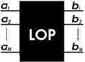
Figure 1: Generic LOP multiport. Horizontal lines represent optical modes entering and leaving the device, from left to right.

The property of photon-number conservation is expressed by the condition:

$$\sum_{i}a^{{\dagger}}_{i}a^{\phantom{{\dagger}}}_{i}=\sum_{i}b^{{\dagger}}_{i}b^{\phantom{{\dagger}}}_{i}\quad.$$ (55)

A simple calculation shows that this condition is sufficient to guarantee that the canonical commutation relations (10) still hold for the operators $\{b^{\phantom{{\dagger}}}_{i},b^{{\dagger}}_{i},\mathbb{I}\}_{i=1}^{N}$, which thus form another basis for the realization of $\mathcal{W}(N)$, and can indeed be interpreted as the field operators of the output modes.
In fact, denoting by $\underline{U}$ the matrix representing the LOP transformation:

$$b^{\phantom{{\dagger}}}_{i}=\sum_{j}\underline{U}_{ij}a^{\phantom{{\dagger}}}_{j}\quad,$$ (56)

from condition (55) one can easily prove that

$$\underline{U}\,\,\underline{U}^{{\dagger}}=\underline{U}^{{\dagger}}\,\underline{U}=\mathrm{Id}\quad,$$ (57)

where Id is the identity matrix. Hence, with any LOP transformation it can be naturally associated a unitary matrix $\underline{U}$; conversely, any unitary matrix defines a LOP transformation. Thus, there is a one-to-one correspondence between LOP $2N$-ports and the elements of the group U($N$).

On the other hand, formula (56) implies that any invariant linear span for the operators $\{b^{\phantom{{\dagger}}}_{i},b^{{\dagger}}_{i}\}_{i=1}^{N}$ must be invariant for the operators $\{a^{\phantom{{\dagger}}}_{i},a^{{\dagger}}_{i}\}_{i=1}^{N}$ as well, and this in turn means that the output field operators $\{b^{\phantom{{\dagger}}}_{i},b^{{\dagger}}_{i}\}_{i=1}^{N}$ form another irreducible set. Thus, as we have already pointed out in §2.1, by the Stone-von Neumann theorem they must be unitarily equivalent to the operators $\{a^{\phantom{{\dagger}}}_{i},a^{{\dagger}}_{i}\}_{i=1}^{N}$, i.e.

$$b^{\phantom{{\dagger}}}_{i}=U^{{\dagger}}a^{\phantom{{\dagger}}}_{i}U\quad,\quad i=1,\ldots,N\quad,$$ (58)

where $U$ is a unitary operator in $\mathscr{H}_{F}^{(N)}$ uniquely defined up to an arbitrary phase factor.

Observe that, as a consequence of the photon-number conservation, the subspaces $\mathscr{H}_{n}^{(N)}\,,\,n=0,1,\ldots$ of $\mathscr{H}_{F}^{(N)}$ are invariant subspaces for the operator $U$. In fact, using the definition of $\hat{n}$ and condition (55), one can easily check that the unitary operator $U$ commutes with $\hat{n}$:

$$U\,\hat{n} = U\,\hat{n}\,U^{{\dagger}}\,U$$ (59)

$$= \left(\sum_{i}U\,b^{{\dagger}}_{i}b^{\phantom{{\dagger}}}_{i}\,U^{{\dagger}}\right)U$$

$$= \sum_{i}a^{{\dagger}}_{i}a^{\phantom{{\dagger}}}_{i}\,U$$

$$= \hat{n}\,U\quad.$$

Then, since $\mathscr{H}_{n}^{(N)}\,,\,n=0,1,\ldots$, is an eigenspace of $\hat{n}$, it must be an invariant subspace for $U$.
In particular, as $\mathscr{H}_{0}^{(N)}=$ span$\{|\mathbf{0}\rangle\}$, we have:

$$U|\mathbf{0}\rangle=e^{i\phi}|\mathbf{0}\rangle\quad,$$ (60)

for some $\phi\in\mathbb{R}$. We will now show that one can give an explicit form of the operator $U$ in such a way that $e^{i\phi}=1$. To this aim, consider the following recipe:

• write the matrix $\underline{U}$ (associated with any LOP $2N$-port) as the exponential of a matrix in the Lie algebra $\mathfrak{u}(N)$:

  $$\underline{U}=e^{i\underline{J}}\quad,\quad\underline{J}\in\mathfrak{u}(N)\quad;$$ (61)

• next, via the J-S map, one can obtain a self-adjoint operator $J$:

  $$J=\mathrm{JS}(\underline{J})=\sum_{ij}\underline{J}_{ij}a^{{\dagger}}_{i}a^{\phantom{{\dagger}}}_{j}\quad;$$ (62)

• eventually one can define a unitary operator

  $$U\doteq\mathrm{exp}(i\mathrm{JS}(\underline{J}))=\mathrm{exp}\big{(}i\sum_{ij}\underline{J}_{ij}a^{{\dagger}}_{i}a^{\phantom{{\dagger}}}_{j}\big{)}\quad.$$ (63)

We now claim that

1. the unitary operator $U$ verifies eq. (56);

2. the definition of $U$ does not depend on the choice of a particular element $\underline{J}$ of the algebra $\mathfrak{u}(N)$ such that exp$(i\underline{J})=\underline{U}$;

3. the matrix $\bar{U}_{1}^{(N)}$ representing the operator $U$ in the one-photon subspace $\mathscr{H}_{1}^{(N)}$ of $\mathscr{H}_{F}^{(N)}$ is $\underline{U}$, precisely:

   $$\langle 0,\ldots,0,\overbrace{1}^{i},0,\ldots,0|\,U\,|0,\ldots,0,\overbrace{1}^{j},0,\ldots,0\rangle=\underline{U}_{ij}\quad.$$ (64)

Indeed, let $\underline{J}$ be a matrix in $\mathfrak{u}(N)$ and let us define the unitary operator $U$ by formula (63). Then, using the well known relation

$$e^{\hat{A}}\,\hat{B}\,e^{-\hat{A}}=\mathrm{exp}(\mathrm{ad}_{\hat{A}})\hat{B}$$ (65)

that holds for generic linear operators $\hat{A},\hat{B}$ (with ad${}_{\hat{A}}\hat{B}\doteq[\hat{A},\hat{B}]$), and applying the canonical commutation relations, one easily proves that

$$U^{{\dagger}}a^{\phantom{{\dagger}}}_{k}U=\sum_{l}(e^{i\underline{J}})_{kl}a^{\phantom{{\dagger}}}_{l}\quad,\quad k=1,\ldots,N\,;$$ (66)

hence, for any $\underline{J}$ satisfying $e^{i\underline{J}}=\underline{U}$, the operator $U$ verifies eq. (56).
Next, we prove that the association $\underline{U}\mapsto{U}$ defined by formula (63) does not depend on the choice of the matrix $\underline{J}$ such that $e^{i\underline{J}}=\underline{U}$. To this aim, observe that — according to the Stone-von Neumann theorem — the operator $U$, which verifies eq. (56), is uniquely identified by the phase factor $e^{i\phi}$ appearing in eq. (60). Now, one can immediately check that, for any matrix $\underline{J}\in\mathfrak{u}(N)$, we have:

$$\mathrm{exp}\Big{(}i\sum_{k,l}\underline{J}_{kl}a^{{\dagger}}_{k}a^{\phantom{{\dagger}}}_{l}\Big{)}|\mathbf{0}\rangle=|\mathbf{0}\rangle\quad;$$ (67)

hence, $e^{i\phi}=1$ for $U$ defined by formula (63) independently on the choice of $\underline{J}$ such that $e^{i\underline{J}}=\underline{U}$. This proves that the definition of $U$ itself does not depend on a particular choice of such a matrix $\underline{J}$, namely, our second claim.
Our third claim can be checked by an elementary calculation, by explicitly evaluating the l.h.s of eq. (64):

$$\langle\mathbf{0}|a^{\phantom{{\dagger}}}_{i}Ua^{{\dagger}}_{j}|\mathbf{0}\rangle = \langle\mathbf{0}|U(U^{{\dagger}}a^{\phantom{{\dagger}}}_{i}U)a^{{\dagger}}_{j}|\mathbf{0}\rangle$$ (68)

$$= \langle\mathbf{0}|b^{\phantom{{\dagger}}}_{i}a^{{\dagger}}_{j}|\mathbf{0}\rangle$$

$$= \sum_{k}\underline{U}_{ik}\langle\mathbf{0}|a^{\phantom{{\dagger}}}_{k}a^{{\dagger}}_{j}|\mathbf{0}\rangle$$

$$= \underline{U}_{ij}\quad.$$

(in the second line we used the fact that $U|\mathbf{0}\rangle=|\mathbf{0}\rangle\,,\,U^{{\dagger}}a^{\phantom{{\dagger}}}_{i}U=b^{\phantom{{\dagger}}}_{i}$). Summarizing, we have shown that with any LOP $2N$-port one can associate in a unique way two mathematical objects:

• a unitary matrix $\underline{U}$ representing the LOP transformation: $b^{\phantom{{\dagger}}}_{i}=\sum_{j}\underline{U}_{ij}a^{\phantom{{\dagger}}}_{j}$;

• a unitary operator $U$ uniquely identified by the equations

  $$b^{\phantom{{\dagger}}}_{i}=U^{{\dagger}}a^{\phantom{{\dagger}}}_{i}U\quad i=1,\ldots,N\quad,\quad U|\mathbf{0}\rangle=|\mathbf{0}\rangle\,.$$ (69)

Moreover, we have shown that one can give an explicit procedure for building the operator $U$ from the matrix $\underline{U}$; conversely, if the operator $U$ is given, then the matrix $\underline{U}$ can be obtained from relation (64).

We conclude observing that the J-S map JS induces a map $\widehat{\mathrm{JS}}\,:$ U($N$) $\rightarrow\mathcal{U}(\mathscr{H}_{F}^{(N)})$ where $\mathcal{U}(\mathscr{H}_{F}^{(N)})$ is the group of unitary operators in $\mathscr{H}_{F}^{(N)}$, defined by:

$$\widehat{\mathrm{JS}}(\underline{U})=\widehat{\mathrm{JS}}(\mathrm{exp}(i\underline{J}))=\mathrm{exp}(i\mathrm{JS}(\underline{J}))=U\quad.$$ (70)

Making use of the Stone-von Neumann theorem one can easily prove that

$$\widehat{\mathrm{JS}}(\underline{U}_{1}\underline{U}_{2})=\widehat{\mathrm{JS}}(\underline{U}_{1})\,\widehat{\mathrm{JS}}(\underline{U}_{2})\quad,$$ (71)

for any $\underline{U}_{1},\underline{U}_{2}\,\in\,$ U($N$), i.e. that $\widehat{\mathrm{JS}}$ is a unitary representation of U($N$).

2.4 Basic examples

Now we give an explicit form to the objects we have introduced so far, namely the matrix $\underline{U}$ and the operator $U$, for two simple special cases: the 2- and the 4-port. They are indeed special because they are the only LOP directly implemented in the labs respectively by phase shifters (PS) and beam splitters (BS); then, any generic linear optical multiport can be implemented decomposing it as an array of 2- and 4-ports  [33].

The simplest example is the PS, the LOP $2$-port (Fig. 2) whose action is just the phase multiplication:

$$b=e^{+i\phi}a\quad,\quad b^{{\dagger}}=e^{-i\phi}a^{{\dagger}}\quad.$$ (72)

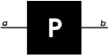
Figure 2: LOP $2$-port: phase-shifter.

The group involved is U(1), and its generator is simply $\underline{J}=1$; in this case, the J-S map associates with $\underline{J}$ the number operator, so that $J=a^{{\dagger}}a$, and:

$$b=P^{{\dagger}}\,a\,P\quad\mathrm{with}\quad P(\phi)=e^{+i\phi\hat{n}}\quad.$$ (73)

Notice that $P$ acts on the Fock space $\mathscr{H}_{F}$ as a photon-number-dependent phase factor.
A generic LOP $4$-port (Fig. 3) is described by the $2\times 2$ unitary matrix $\underline{B}$  [34, 35]:

$$\underline{B}=e^{i\phi_{0}}\underline{B}^{\prime}=e^{i\phi_{0}}\left(\begin{array}[]{cc}e^{i\phi_{\tau}}\cos\theta&e^{i\phi_{\rho}}\sin\theta\\ -e^{-i\phi_{\rho}}\sin\theta&e^{i\phi_{\tau}}\cos\theta\end{array}\right)\quad;$$ (74)

the $4$-port is implemented by PSs and BSs, respectively corresponding to the U(1) factor and the SU(2) matrix $B^{\prime}$.

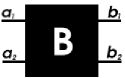
Figure 3: LOP $4$-port: beam-splitter.

To obtain the operator representation of the BS’s SU(2) matrix, we consider the well-known Euler decomposition of a generic SU(2) matrix as the product of three elementary ’rotations’; then, recalling the bosonic realization of the $\mathfrak{su}(2)$ generators $J_{k}$, and the induced map $\widehat{\mathrm{JS}}$, we can write:

$$B^{\prime}(\alpha,\beta,\gamma)=e^{-i\gamma J_{z}}e^{-i\beta J_{y}}e^{-i\alpha J_{z}}\quad,$$ (75)

where $J_{i}=$JS$(\frac{1}{2}\sigma_{i})$ are the linear combinations of the operators $\{a^{{\dagger}}_{i}a^{\phantom{{\dagger}}}_{j}\}_{i,j=1}^{N}$ given by equations (2.2).

3 LOP schemes for deterministic quantum computation

In this section we apply the results of §2.2, 2.3 and derive a constructive procedure for building LOP circuits for deterministic quantum computation on an arbitrary number of qubits; then we discuss the issue of scalability.

3.1 Encoding: the SPMQ scheme

The encoding of (quantum) information is generally made possible by a more or less strict correspondence between the mathematical properties of the symbols that are chosen to represent the information, and those of the description of the physical system that is chosen to encode symbols. The case of the SPMQ encoding is special from this point of view, since such a correspondence is indeed a complete equivalence in this case.
As we have already said, symbols in quantum information are represented by qu$N$its; universal quantum computation can be done on strings of qubits in the common case of the binary coding. It is useful to recall the following abstract definitions:

• a quNit is a vector in a $N$-dimensional abstract Hilbert space, endowed with the fundamental representation of U($N$) acting on it;

• a string of k qubits, or k-qubit, is a vector in a $2^{k}$-dimensional Hilbert space — specifically the tensor product of $k$ copies of the 2-dimensional single qubit Hilbert space — endowed with the fundamental representation of U(2^k) acting on it.

It should be clear from the results of §2.2 that the mathematical characterization of $\mathscr{H}_{1}^{(N)}$ — the space of the states of a single photon over $N$ optical modes — perfectly fits with the abstract definition of the qu$N$it space; furthermore, chosing $N=2^{k}$, one can say that $\mathscr{H}_{1}^{(2^{k})}$ concides with the previous abstract definition of the Hilbert space of a string of $k$ qubits.
The SPMQ encoding is the one-to-one correspondence between logical states — i.e. the states of a string of k abstract qubits — and the physical states — i.e. the states of the quantum system of a single photon over $2^{k}$ modes. The correspondence between logical and physical states can be formulated explicitly, using te well known computational basis notation: if we denote by $\{|\mathtt{i}\rangle\}_{i=1}^{2^{k}}$ the states of a given basis of the k logical qubits, we can rewrite them as column vectors with $2^{k}$ elements, that are all zero except for a 1 in the $i$-th position, with $i=1,\ldots,2^{k}$. Then, the SPMQ scheme consists in encoding the logical state $|\mathtt{i}\rangle$ by the state of one photon in the $i$-th mode, with $i=1,\ldots,2^{k}$, and the corresponding notation is:

$$\mathrm{logicalstates} \longleftrightarrow \mathrm{physicalstates}$$

$$|\mathtt{i}\rangle\equiv\left(\begin{array}[]{c}0\\ \vdots\\ 0\\ 1\\ 0\\ \vdots\\ 0\end{array}\right)\}i \longleftrightarrow |0\ldots 0\overbrace{1}^{i}0\ldots 0\rangle=a^{{\dagger}}_{i}|\mathbf{0}\rangle\,.$$ (83)

3.2 Elaboration: the algebraic scheme

We now claim that with this encoding scheme, LOP devices are sufficient to implement deterministically any quantum circuit, without the need for ancillary resources and postselection schemes  [2].

As we have previously shown, with any LOP $2N$-port one can associate a matrix in U($N$) acting on the input modes $a^{\phantom{{\dagger}}}_{1},\ldots,a^{\phantom{{\dagger}}}_{n}$, or equivalently a unitary operator $U$ acting ’by similarity’: $a^{\phantom{{\dagger}}}_{k}\,\mapsto\,U^{{\dagger}}a^{\phantom{{\dagger}}}_{k}U$. From the physical point of view, this is nothing but the action of the time evolution operator associated with the $2N$-port (regarded as a quantum device) on the input field operators in the ’Heisenberg picture’.
On the other hand, as far as applications to QIP and QC are concerned, since the encoding resource is given by the state vectors of the Fock space, it is convenient to switch to the ’Schr’́odinger picture’ and to represent the action of the LOP devices (regarded as quantum logic gates) as the action of the associated unitary operators on the state vectors. The operator $U$ can be represented by an infinite unitary matrix, after choosing a labeling of the Fock states; now we are interested in the action of $U$ on the subspace $\mathscr{H}_{1}^{(N)}$, and, as shown in (68), this is represented by a U($N$) matrix $\bar{U}_{1}^{(N)}$ wich coincides with $\underline{U}$. Since we know that any U($N$) matrix $\underline{U}$ corresponds to a LOP $2N$-port built from an array of BS and PS  [33], this means that we can act on $\mathscr{H}_{1}^{(N)}$ with any desired unitary transformation, and so we can do any quantum computation on a string of a fixed number of qubits.
To make the last statement more precise, once again we refer to the computational basis notation: recall that any logical quantum circuit acting on input strings of $k$ logical qubits is represented by some unitary operator $C$ acting on the $k$-qubit Hilbert space. After chosing a basis $\{|\mathtt{i}\rangle\}_{i=1}^{2^{k}}$ for the logical states, the operator $C$ associated with the circuit can be represented by a $2^{k}\times 2^{k}$ unitary matrix on such a basis:

$$(C)_{ij}\doteq\langle\mathtt{i}|C|\mathtt{j}\rangle\quad;$$ (84)

this is the computational basis matrix of the quantum circuit.
Then, when using the SPMQ encoding, in order to design the LOP circuit which implements a given $k$-qubit quantum circuit, one just needs to follow three simple steps:

1. write down the computational basis matrix of the logical circuit;

2. take the $(C)_{ij}$ as the matrix elements of the $\bar{U}_{1}^{(N)}=\underline{U}$ matrix of a LOP circuit;

3. apply the RZBB procedure ˜[33] to decompose the $\underline{U}$ matrix in the corresponding array of PS’s and BS’s.

This simple, constructive procedure for designing LOP quantum circuits constitutes the demonstration of the claim we made at the beginning of this section.

To conclude, notice that the simplicity of the procedure we presented makes it suitable for translation into an algorithm that could be run by a classical computer; furthermore, if BS and PS with variable parameters were available, being their maximum number fixed by the number of modes $N$, LOP components could be rearranged automathically in the appropriate configuration, thus making the design of LOP quantum circuit a comletely authomatized process.

3.3 The issue of scalability

LOP circuits for deterministic quantum computation can be designed when encoding strings of qubits by single photon multimode states; but there are two practical problems related to this scheme.

1. The first one is the fact that, in order to encode a $k$-qubit state, we need $2^{k}$ optical modes, which means that an exponential amount of physical resource is required; this limits the practical feasibility of circuits acting on an arbitrary number of qubits.

2. On the other hand, this scheme is deterministic only for computations executed on a fixed number of qubits: when coupling two registers, physical states of 2 photons will appear, which do not encode any logical state. Consider two strings of $k_{1}$ and $k_{2}$ qubits; these are encoded respectively on the spaces $\mathscr{H}_{1}^{(N_{1})}$ and $\mathscr{H}_{1}^{(N_{2})}$, where $N_{i}=2^{k_{i}}$. The resulting physical system after a generic LOP is the system of two photons on $N_{1}+N_{2}$ modes, whose Hilbert space $\mathscr{H}_{2}^{(N_{1}+N_{2})}$ is strictly larger than the encoding space $\mathscr{H}_{1}^{(N_{1})}\otimes\mathscr{H}_{1}^{(N_{2})}$.

At present stage it is not clear yet what the architecture of a quantum computer will be, but it seems reasonable that it will be a hybrid object made out of different components; in this regard, scalability is only one of the requirements to be satisfied, and it should not be considered so stringent as to rule out a proposal for the implementation. With the scheme we presented here, one can build circuits acting on a small number, e.g. 2 or 3, of qubits, which allow to test experimentally with present technology some interesting QIP protocols, as we show in the next section. As a further remark, we just point out a possible way to reduce the number $N$ of optical modes necessary to encode $k$-qubit logical states, in such a way that $N$ is polynomial in $k$. In fact, one could encode $k$-qubits in the subspace $\mathscr{H}_{n}^{(N)}$ of $\mathscr{H}_{F}^{(N)}$, with $n\geq 2$, and suitably exploit the irreducible representations of U($N$) acting in such subspaces for implementing logic gates.

With respect to the second problem, a solution could be found by means of a suitable postselected circuit that allows to reduce this deterministic non-scalable scheme to the non-deterministic scalable scheme proposed in  [2], and viceversa.

4 2-qubit deterministic circuits

We first give some basic examples of 2-qubit gates, and then a composite circuit for the generation and measurement of Bell states. To this aim, we write down explicitly the linear map that encodes logical 2-qubit states by single-photon 4-mode states, namely on $\mathscr{H}_{1}^{(4)}$:

$$\begin{array}[]{ccccc}\mathrm{logicalstates}&{}\hfil&\mathrm{binaryform}&{}\hfil&\mathrm{physicalstates}\\ |\mathtt{1}\rangle&\longleftrightarrow&|\mathtt{00}\rangle&\longleftrightarrow&|1000\rangle\\ |\mathtt{2}\rangle&\longleftrightarrow&|\mathtt{01}\rangle&\longleftrightarrow&|0100\rangle\\ |\mathtt{3}\rangle&\longleftrightarrow&|\mathtt{10}\rangle&\longleftrightarrow&|0010\rangle\\ |\mathtt{4}\rangle&\longleftrightarrow&|\mathtt{11}\rangle&\longleftrightarrow&|0001\rangle\\ \end{array}$$ (85)

where, following the conventional notation for $k$-qubit states, in the central column we have introduced the binary form of the logical state; we will always use this notation in what follows.

4.1 cNOT

The first LOP circuit we present is a very simple one, implementing a cNOT gate. This is a 2-qubit universal gate, i.e. it can be shown that the cNOT and arbitrary 1-qubit gates are sufficient to build any quantum logic network. The cNOT gate acts on the logical computational basis states flipping the second (target) qubit when the first (control) qubit is in the state $|\mathtt{1}\rangle$:

$$|\mathtt{00}\rangle \mapsto |\mathtt{00}\rangle$$

$$|\mathtt{01}\rangle \mapsto |\mathtt{01}\rangle$$

$$|\mathtt{10}\rangle \mapsto |\mathtt{11}\rangle$$

$$|\mathtt{11}\rangle \mapsto |\mathtt{10}\rangle$$ (86)

and it is represented by the following matrix acting on the computational basis vectors:

$$cNOT=\left(\begin{array}[]{cccc}1&0&0&0\\ 0&1&0&0\\ 0&0&0&1\\ 0&0&1&0\end{array}\right).$$ (87)

Exploiting the following matrix identity:

$$cNOT=\bar{U}_{1}^{(4)}=\underline{U}$$ (88)

one can buid the LOP circuit (Fig. 4) corresponding to $\underline{U}$: decomposition  [33] is trivial in this case, since $\underline{U}$ itself describes the transformation of a BS with $100\%$ transmission (that is, a simple exchange) coupling modes 3 and 4. Note that only one single photon source, three vacuum sources, and a classically controllable operation (the interchange of modes 3 and 4) are required, thus eliminating a possible source of errors due to non-ideal LOP components; the simplicity of this circuit is remarkable if one thinks that the cNOT is a basic gate that could be applied several times while running a quantum computation.

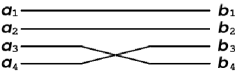
Figure 4: LOP cNOT.

4.2 cPHASE

This gate append a desired phase facor $e^{-i\phi}$ to the state $|\mathtt{11}\rangle$, while leaving the other unchanged; it can be shown by a simple calculation that a cNOT transformation can be obtained by a cPHASE with $\phi=\pi$ (also called cSIGN) preceeded and followed by a suitable transformation of the target qubit.

The cPHASE is represented by the matrix:

$$cPHASE=\left(\begin{array}[]{cccc}1&0&0&0\\ 0&1&0&0\\ 0&0&1&0\\ 0&0&0&e^{-i\phi}\end{array}\right)\quad;$$ (89)

also in this case decomposition is trivial, and the corresponding LOP circuit requires only one PS with $\phi=\pi$ acting on the 4-th mode, as depicted in Fig. 5.

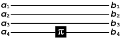
Figure 5: LOP cPHASE.

4.3 SWAP gate

This is the gate that interchanges the logical state of the two qubits, represented by the matrix:

$$SWAP=\left(\begin{array}[]{cccc}1&0&0&0\\ 0&0&1&0\\ 0&1&0&0\\ 0&0&0&1\end{array}\right)$$ (90)

and it correspond to a sequence of three alternate cNOT’s. But within this scheme it is not necessary to implement this sequence: it suffices to note that the $SWAP$ matrix interpreted as a LOP matrix describes a BS with $100\%$ transmission coupling modes 2 and 3, which corresponds to the simple circuit shown in Fig. 6.

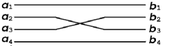
Figure 6: LOP SWAP.

4.4 Bell states production and analysis

Many QIP protocols, e.g. quantum teleportation  [39], rely on the use of entangled states of qubits as a resource, and on the ability to distinguish among such states, thus leading to many efforts towards the production and detection of entangled physical states. Bell states are defined as the four maximally entangled states of a 2-qubit system; within the scheme of QC they can be produced by means of a circuit composed by a cNOT preceeded by a Hadamard gate on the control qubit: this maps the logical computational basis states onto the Bell states:

$$|\mathtt{00}\rangle \mapsto \frac{|\mathtt{00}\rangle+|\mathtt{11}\rangle}{\sqrt{2}}$$

$$|\mathtt{01}\rangle \mapsto \frac{|\mathtt{01}\rangle+|\mathtt{10}\rangle}{\sqrt{2}}$$

$$|\mathtt{10}\rangle \mapsto \frac{|\mathtt{00}\rangle-|\mathtt{11}\rangle}{\sqrt{2}}$$

$$|\mathtt{11}\rangle \mapsto \frac{|\mathtt{01}\rangle-|\mathtt{10}\rangle}{\sqrt{2}}$$ (91)

By a simple calculation one finds that it is represented by the followng matrix:

$$cNOT\cdot(H_{1}\otimes\mathbb{I}_{2})=\left(\begin{array}[]{cccc}\frac{1}{\sqrt{2}}&0&\frac{1}{\sqrt{2}}&0\\ 0&\frac{1}{\sqrt{2}}&0&\frac{1}{\sqrt{2}}\\ 0&\frac{1}{\sqrt{2}}&0&-\frac{1}{\sqrt{2}}\\ \frac{1}{\sqrt{2}}&0&-\frac{1}{\sqrt{2}}&0\end{array}\right)$$ (92)

where $H$ denotes the Hadamard gate, and index 1 refers to the fact that it acts on the first (control) qubit.

Implementation of a Bell state analyzer in the framework of linear optics has been studied  [36, 37, 38] leading to the result that a complete measurement in the qubit polarization Bell basis is not possible. Nevertheless, in the SPMQ scheme we are proposing, a simple LOP circuit for the simulation of Bell state production and analysis can be found that works deterministically: as in the previous examples, one just takes the matrix (92) as a LOP circuit matrix, decompose it and obtain the circuit depicted in Fig. 7. Only two balanced ($50\%$ transmission) BS, with a sign change upon reflection off the lower side, and interchange of modes 3 and 4 are required.

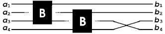
Figure 7: LOP circuit for Bell states generation (running from left to right) and measurement (from rigtht to left). The two BS are balanced, and produce a sign change on reflection off the lower face.

5 Conclusions and perspectives

In this paper we have considered some algebraic structures of linear optics, and discussed how they provide a natural way to deal with Linear-Optical Quantum Computing; on the other hand, we have stressed on the correspondence of such algebraic objects with the basic instruments used in the laboratories, to point out that practical implementations can, in principle, be designed and tested.

As a result, we first derived a SPMQ scheme for encoding any number of qubits by only one photon; then, we described an algorithmic procedure which, given any logical quantum circuit, allows to design the linear optical circuit which implements the logical circuit operation deterministically, and we presented some simple but interesting $2$-qubit gates and circuits.

We also discussed some practical problems related to the scalability of such scheme, and pointed out some possible solutions. However it seems reasonable that in the future a quantum computer will be a composite object, which will exploit either scalable and non-scalable, either deterministic and non-deterministic components (most likely in association with classical components).

In this regard, it is interesting to test such components experimentally, and further work is to be done to quantify the effects of non-ideal instruments on the theoretical schemes. It should be noticed that the scheme proposed here requires no ancillary systems, namely additional photon sources and counters, which are the main sources of inefficiency; only one single photon source is required, regardless of the number of qubits, and this should lead to an efficiency which is almost independent on the number of qubits.

References

References

- [1] See Nielsen M and Chuang I 2000 ”Quantum Information and Quantum Computation” (Cambridge University Press) and references therein.
- [2] Knill E, Laflamme R and Milburn G 2001 Nature (London) 409 46
- [3] Scheel S, Nemoto K, Munro W J, and Knight P L 2003 Phys. Rev. A 68 032310
- [4] Lapaire G G, Kok P, Dowling J P, and Sipe J S 2003 Phys. Rev. A 68 042314
- [5] Clausen J, Knoll L, and Welsch D G 2003 Phys. Rev. A 68 043822
- [6] Pittman T B, Jacobs B C, and Franson J D 2001 Phys. Rev. A 64 062311
- [7] Ralph T C, White A G, Munro W J, and Milburn G J 2001 Phys. Rev. A 65 012314
- [8] Ralph T C, Langford N K, Bell T B, and White A G 2002 Phys. Rev. A 65 062324
- [9] Lund A P, and Ralph T C 2002 Phys. Rev. A 66 032307
- [10] Knill E 2002 Phys. Rev. A 66 052306
- [11] Dodd J L, Ralph T C, and Milburn G J 2003 Phys. Rev. A 68 042328
- [12] Giorgi G L, de Pasquale F, and Paganelli S 2004 Phys. Rev. A 70 022319
- [13] Pittman T B, Fitch M J, Jacobs B C, and Franson J D 2003 Phys. Rev. A 68 032316
- [14] Sanaka K et al. 2003 Nature (London) 421 721-724
- [15] O’Brien J L et al. 2003 Nature (London) 426 264
- [16] Pittman T B, Jacobs B C, and Franson J D Preprint quant-ph/0404059
- [17] Gasparoni S et al. Preprint quant-ph/0404107
- [18] Zhao Z et al. Preprint quant-ph/0404129
- [19] Sanaka K et al. 2004 Phys. Rev. Lett. 92(1)
- [20] Milburn G J 1988 Phys. Rev. Lett. 62 2124
- [21] Cerf N J, Adami C, and Kwiat P G 1998 Phys. Rev. A 57 R1477
- [22] Englert B G, Kurtsiefer C, and Weinfurter H 2003 Phys. Rev. A 63 032303
- [23] Fiorentino M, Kim T, and Wong F N C Preprint quant-ph/0407136
- [24] Fiorentino M, and Wong F N C 2004 Phys. Rev. Lett. 93 070502
- [25] This condition — that appears in a remarkable paper by Dixmier J 1958 Comp. Math. 13 263-270 — allows to rule out possible non-standard (i.e. inequivalent) realizations of the canonical commutation relations; as an example of such a non-standard (but physically meaningful) realization, see Reeh H 1988 J. Math. Phys. 29 1535-1536 .
- [26] Stone M H 1930 Proc. Nat. Acad. Scie. U.S.A. 16 172-175
- [27] von Neumann J 1931 Math. Ann. 104 570-578
- [28] Jordan P 1935 Z. Phys. 94 531
- [29] Schwinger J 1965 in ”Quantum theory of angular momentum” L.C. Biedenharm and H. Van Dam eds (Academic Press)
- [30] Man’ko V I, Marmo G, Vitale P, and Zaccaria F 1994 Int. J. Mod. Phys. A9 5541
- [31] Wunsche A 2000 Quantum Semiclass. Opt. 2 73-80
- [32] Simon B 1996 ”Representations of Finite and Compact Groups”, Graduate Studies in Mathematics 10 (AMS)
- [33] Reck M, Zeilinger A, Bernstein H J, and Bertani P 1994 Phys. Rev. Lett. 73 58
- [34] Yurke B, McCall S L, and Klauder J R 1986 Phys. Rev. A 33 4033
- [35] Campos R A, Saleh B E A, and Teich M C 1989 Phys. Rev. A 40 1371
- [36] Lutkenhaus N, Calsamiglia J, and Suominen K A 1999 Phys. Rev. A 59 3295
- [37] Calsamiglia J and Lutkenhaus N 2001 Appl. Phys. B 59 67
- [38] Lutkenhaus N, Calsamiglia J, and Suominen K A 2002 Phys. Rev. A 65 030301(R)
- [39] Bennett C H et al. 1993 Phys. Rev. Lett. 70 1895