Electron-nuclear entanglement in the cold lithium gas
Abstract
We study the ground-state entanglement and thermal entanglement in the hyperfine interaction of the lithium atom. We give the relationship between the entanglement and both temperature and external magnetic fields.
keywords:
Entanglement , Cold atom gasPACS:
03.65.Ud , 03.75.Gg1 Introduction
Quantum entanglement is an important prediction of quantum mechanics and constitutes indeed a valuable resource in quantum information processing. In recent years, many important results have been obtained in both experimental and theoretical aspects[1].
The effects of the temperature were taken into account and some authors used thermal entanglement to study the electron spin system or other models at finite temperature in Refs.[2, 3, 4]. For example, X.G. Wang investigated the isotropic Heisenberg XXX model at finite temperature[3]. Y. Sun et al. investigated the thermal entanglement in the two-qubit Heisenberg XY model in nonuniform magnetic fields[4]. On the other hand, the entanglement at the critical point is also a hot point[5, 6]. For instance, Osterloh et al. demonstrated that for a class of one-dimensional magnetic systems, that entanglement shows scaling behavior in the vicinity of the transition point[5]
In this paper, we study the entanglement in the atom. Near absolute zero, the atom will show some particular properties. As we know, in atom the 3 electrons possess spin and the nucleus has 3 protons and 3 neutrons so that the total nuclear spin is . Because the number of neutrons is odd, the atom obeys fermion statistics. As we know, two research groups have succeeded in producing a Bose-Einstein condensation of molecules made from pairs of fermion atoms[7, 8]. Note that the atoms are fermions but if considered as pairs they are bosons and therefore able to condense in Bose-Einstein fashion. So it is necessary to study the entanglement properties of the atom in the external fields at very low temperature.
In the following, the ground state entanglement of such a system is evaluated by means of the method of Rungta’s concurrence. Then we use negativity to study the entanglement between the electrons and the nucleus at finite temperature.
2 The model and Hamiltonian
In the atom, the electron spins are coupled to the nuclear spin by the hyperfine interaction. The hyperfine line for the lithium atom has a measured magnitude of 228MHz in frequency. Some calculation on the basis of first-order perturbation for the magnetic dipole interaction between the electron and the nucleus gives contribution to the coupling strength of term. In this paper, we study a bipartite system, one is the nucleus which has the spin- and the other is the electron which has total spin-. The both parts are interacted with different external magnetic fields, and . Since the electrons have no orbital angular momentum(), there is no magnetic field at the nucleus due to the orbital motion. The Hamiltonian can be written as follows,
| (1) |
where J is the coupling constant. Throughout the paper, the constant is set to unit. is the nuclear spin which has spin-1 and is electron spin. The two parameters are related to the external fields. They are given by
| (2) |
In the Hamiltonian (1) the electronic orbital angular momentum has been assumed to be zero. For the lithium atom, the nuclear magnetic moment , where . Since , for most applications D can be neglected. At the same level of approximation the factor of the electron may be put equal to 2[9]. In this paper, the spin-1/2 state has the bases as , and the spin-1 state has the bases as , , . In the above bases, the Hamiltonian can be rewritten as follows,
| (3) |
From the Hamiltonian one can easily obtain the eigenvalues and eigenvectors. During the evaluation of the entanglement of the system, we will have to deal with the high-dimensional Hilbert space. Rungta et al. raised a quantity they called it I concurrence to measure the high-dimensional bipartite pure state[10]. The quantity is given by
| (4) |
where and are the dimensions of the Hilbert spaces and are two parameter related to dimension. Here they can be set to unit. is the reduced density matrix. The concurrence vanishes for unentangled state. Let . So the concurrence arranges from 0 to .
3 Entanglement in the presence of non-uniform fields
In this section, we will study the ground-state entanglement of the system. Since the parameter is much larger than , D will be neglected.
(a) When , the ground state energy is and the eigenvector is given by
| (5) |
where is the normalization factor. One can use Rungta’s concurrence to measure the entanglement and obtain
| (6) |
(b) When , the ground state is and the eigenvector is given by
| (7) |
where is the normalization factor. The concurrence is
| (8) |
The above results can be plotted in Fig.2 and Fig.2. Fig.2 shows the relationship between the ground-state energy and external magnetic fields. Fig.2 shows the relationship between the ground-state entanglement and external magnetic fields C.


From the Fig.2, one can see when the parameter approaches zero, i.e., the magnetic fields is vanishing, the concurrence approaches its maximum In fact, when the magnetic field is absent, the ground state is degenerate, it will be discussed in the following paragraph.
(c) When , i.e. the magnetic field is absent, the ground state will be double degenerate. As we know, if the ground state is degenerate the zero-temperature ensemble becomes an equal mixture of all the possible ground states[6]. In this case, the thermal ground state may be written
| (9) |
where
One can use Negativity to measure the entanglement of the state. The Negativity was introduced by G. Vidal et al[11]. The quantity is given by
| (10) |
where the trace norm is defined by and denotes the partial transpose of the bipartite mixed state . Negativity vanishes for unentangled states. It is easy to know that Negativity of the state (9) is .
4 Thermal entanglement
As we know, since thermal entanglement was introduced in 1998[2], many efforts are devoted to study the thermal state of qubit system. Here we want to use Negativity to study the thermal entanglement of mixed-spin bipartite system at finite temperature.
Here stands for the Gibbs density operator, , where is the partition function, H is the Hamiltonian, T is temperature and is Boltzmann’s constant which we henceforth will set equal to unit. In the bases , , , , , , the thermal state can be rewritten as follows,
| (11) |
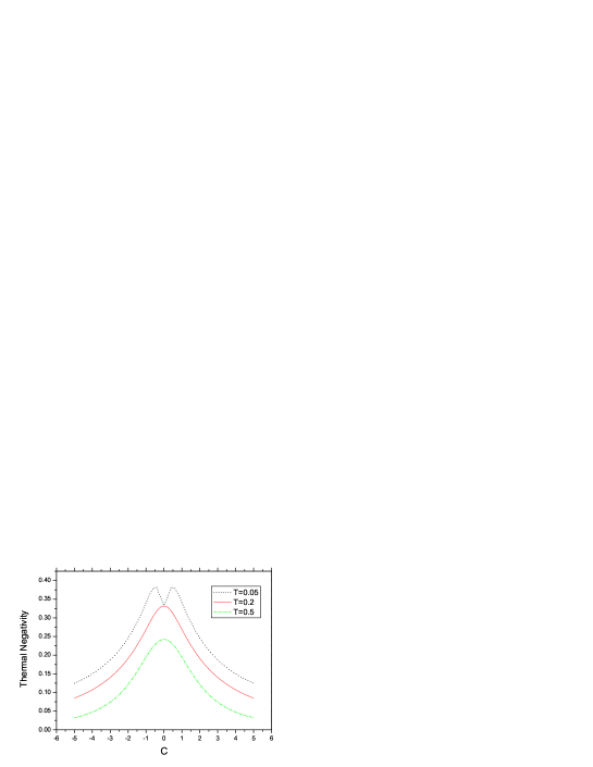
One can use Negativity to study the thermal entanglement of the state. Here the parameter is also neglected. At various temperatures, the Negativity versus can be plotted in Fig.3. From this, one can find when the temperature is low enough, at the point , the Negativity curve has a local minimum. However, as the temperature increases and when it is larger than a critical value , the local minimum changes to be a local maximum. In detail, when , at the point , the Negativity is 0.243. This is a local maximum. When , the Negativity is 0.333, but it is a local minimum. One can see that the temperature can efficiently affect the entanglement of the system.
5 Summary and acknowledgements
In this paper, we studied the entanglement of the electron-nuclear entanglement of atom in presence of uniform external magnetic fields. We studied the ground-state entanglement at zero temperature and thermal entanglement at finite temperature respectively. We gave the relationship between the entanglement and the magnetic fields or temperature. In order to detect the entanglement of the system, the surrounding temperature should be near absolute zero.
This work was supported by NSFC No. 10225419 and 90103022.
References
- [1] M.A. Nielsen and I.L. Chuang, Quantum Computation and Quantum Information, Cambridge University Press, Cambridge, England, 2000
- [2] M.C. Arnesen, S. Bose, V. Vedral, Phys. Rev. Lett. 87(2001) 017901
- [3] X.G. Wang, Phys. Rev. A 66(2002)034302
- [4] Y. Sun, Y.Q. Chen, and H. Chen, Phys. Rev. A 68 (2003), 044301.
- [5] A. Osterloh, L. Amico, C. Falci and G. Fazio,R, Nature(London) 416(2002) 608
- [6] T.J. Osborne and M. Nielsen, Phys. Rev. A 66(2002) 032110
- [7] S. Jochim, M. Bartenstein, A. Altmeyer, G. Hendl, S. Riedl, C. Chin, J. Hecker Denschlag, and R. Grimm, Science 302(2003) 2101
- [8] C. A. Regal, C. Ticknor, J. L. Bohn, and D. S. Jin, Nature 424(2003), 47
- [9] C.J. Pethick, H. Smith, Bose-Einstein Condensation in Dilute Gases, Cambridge Press, Cambridge, 2002
- [10] P. Rungta, V. Buzek, C.M. Caves, M. Hillery, G.J. Milburn, and W.K. Wootters, Phys. Rev. A 64(2001) 042315
- [11] G. Vidal and R.F. Werner, Phys. Rev. A 65(2002) 032314