Hypercomputability of Quantum Adiabatic Processes:
Facts versus Prejudices

Abstract.

We give an overview of a quantum adiabatic algorithm for Hilbert’s tenth problem, including some discussions on its fundamental aspects and the emphasis on the probabilistic correctness of its findings. For the purpose of illustration, the numerical simulation results of some simple Diophantine equations are presented. We also discuss some prejudicial misunderstandings as well as some plausible difficulties faced by the algorithm in its physical implementations.

1. Introduction and outline of the paper

Quantum computation has attracted much attention and investment lately through its theoretical potential to speed up some important computations as compared to classical Turing computation. The most well-known and widely-studied form of quantum computation is the (standard) model of quantum circuits [36] which comprise several unitary quantum gates (belonging to a set of universal gates), arranged in a prescribed sequence to implement a quantum algorithm. Each quantum gate only needs to act singly on one qubit, the generalisation of the classical bit, or on a pair of qubits.

In view of this promising potential of quantum computation, another question that then inevitably arises is whether the class of Turing computable functions can be extended by applying quantum principles. This kind of computation beyond the Turing barrier is also known as hypercomputation [12, 37, 38]. Initial efforts have indicated that quantum computability is the same as classical computability [4]. However, this negative conclusion is only valid for the standard quantum computation. And we know that such a standard model is not the only model of quantum computation. Nor does it necessarily exploit fully the principles of quantum mechanics.

As an illustration of the ability of quantum mechanics, a truly random sequence of bits could be easily generated from a qubit initially prepared in a certain state, while Turing machines have to be content with only pseudo-random generators (see, for example, [51]). (Thus, it seems from the view point of Algorithmic Information Theory [9] that a finitely prepared qubit can have an infinite algorithmic informational theoretic complexity as compared to any finite Turing machine!) This ability to generate random numbers could thus be defined as a form of hypercomputation – albeit of very limited application and of a nature which is non-harnessible or non-exploitable for universal computation.

Also, not restricted by the standard model of quantum computation, we have claimed [24, 25, 26, 27, 29] to have a quantum algorithm for Hilbert’s tenth problem [32] despite the fact that the problem has been proved to be recursively noncomputable. The algorithm makes essential use of the Quantum Adiabatic Theorem (QAT) [34] and other results in the framework of Quantum Adiabatic Computation (QAC) [19], subject to some predetermined and arbitrarily small probability of inaccuracy. We name this kind of algorithms Probabilistically Correct Algorithms to emphasise the fact that the end results from such algorithms are subject to some probabilities of being incorrect. Such error probabilities are necessary when there is, in principle, no other way to verify all the outcomes of the algorithms.

QAC represents another model of quantum computation, alternative to the standard model, and recent studies indicate that QAC offers certain advantages in error and decoherence control [11] and in experimental realisation via quantum optical implementations [31]. More interestingly, the application of QAC to infinite-dimension or unbounded spaces has the potential to extend the classical notion of computability, that is, potential for hypercomputation, through a positive resolution of the Turing halting, Hilbert’s tenth and associated recursively noncomputable problems. For some 70 years many have speculated on some possible extensions of the notion of Church-Turing computability [12]. The recognition of probabilistic quantum physics as the missing ingredients may now be the key for such achievement.

In the next Section we introduce Hilbert’s tenth problem and its equivalence to the Turing halting problem together with their finitely refutable, but Turing noncomputable, characters. Then we collect in the following Section the key ingredients of our proposed quantum adiabatic algorithm for Hilbert’s tenth problem. Emphasis will be put on the probabilistically correct nature of the algorithm and how this nature could evade the no-go results stemmed from Cantor’s diagonal arguments (see [41], for example).

For illustration purposes, we present in Section 4 some numerical simulation examples employing the algorithm with speculation how the infiniteness of the underlying Hilbert space could be probabilistically handled on finite Turing machines. We then move on to a discussion of the misunderstandings or prejudices that we know of, and some potential problems in the physical implementation of the algorithm. The paper concludes with some remarks.

2. Hilbert’s tenth problem and its significance

2.1. Hilbert’s tenth problem

In 1900, David Hilbert presented a list of important problems for the mathematicians of the coming twentieth century. Of twenty three problems on the list, there was only one decision problem (entcheidungsproblem) and also the only one that was not given a name. Ever since it has been called Hilbert’s tenth problem [32], being its position on the list,

Definition 2.1.

(Hilbert’s tenth problem) Given any polynomial equation with any number of unknowns and with integer coefficients: To devise a universal process according to which it can be determined by a finite number of operations whether the equation has (non-negative) integer solutions.

The polynomial equations in question are also called Diophantine equations, some examples of which are the ones involved in Fermat’s last theorem, the most celebrated and well known problem of number theory. Clearly, the availability of such a procedure in the problem of Definition (2.1) is more than a convenience; it would also simplify mathematics and at the same time remove some of the creativeness required of mathematicians for different Diophantine equations. Indeed, if the universal procedure Hilbert asked for is available, many important mathematical problems and conjectures would be exposed and settled by a single mechanical procedure. These are the problems and conjectures which have some Diophantine representations and whose truth values depend on the existence or the lack of (non-negative) integer solutions of the characteristic Diophantine equations. Important examples of these include [7]:

• The Four-Colour Problem: Whether only four colours are sufficient to colour a world map in such a way that no two adjacent countries share the same colour.

• The Goldbach conjecture: Any positive even number can be written as the sum of two primes.

• The Riemann Hypothesis involving the distribution of (non-trivial) zeros of the Riemann zeta function. Determination the truth value of this conjecture is considered by some to be the most important problem of contemporary mathematics.

Associated with each of the above example is a (complicated) Diophantine equation, from which the determination of the truth value for the conjecture is reduced simply to the determination of whether the corresponding equation has a solution or not – a task which could be made much simpler mechanically with Hilbert’s wish.

The significance of Hilbert’s tenth problem is not only limited to the above. It is intimately linked to the formalisation of mathematics (a dream harboured by Leibnitz [15, 10] in the seventeenth century and later by Hilbert himself), a dream which was shattered by Gödel’s incompleteness theorem and, later, the Turing halting theorem. When proposing the tenth problem in 1900, Hilbert himself never anticipated the link it would have with what is the Turing halting problem of the yet-to-be-born field of Theoretical Computer Science. The Turing halting problem was only introduced and solved in 1937 by Turing, and the equivalence of the two problems was not established until 1972 [32], culminating the efforts of three generations of mathematicians.

2.2. Turing halting theorem

The question of the Turing halting problem concerns whether there exists a universal process according to which it can be determined by a finite number of operations if any given Turing machine would eventually halt (in finite time) starting with some specific input. Turing raised this problem in parallel similarity to the Gödel’s Incompleteness Theorem and showed that there exists no such recursive universal procedure. His proof is based on Cantor’s diagonal arguments, also employed in the proof of the Incompleteness Theorem.

The proof is by contradiction, starting with the assumption that there exists a Turing computable halting function $h(p,i)$ which accepts two integer inputs: $p$, the Gödel encoded integer for the Turing machine in consideration, and $i$, the Gödel encoded integer for the input for $p$,

(2.3) $$h(p,i) = \left\{\begin{tabular}[]{l}0 \mbox{ if $p$ halts on input $i$};\\ 1 \mbox{ otherwise}.\end{tabular}\right.$$

One can then construct a program $Turing(n)$ having one integer argument $n$ in such a way that it calls the function $h(n,n)$ as a subroutine and then halts if and only if $h(n,n)=1$. In some made-up language:

	Program $Turing$
	input $n$
10	call $h(n,n)$
	if $h(n,n)=0$ goto 10
	stop
	end

Let $t$ be the Gödel encoded integer for the program $Turing$; we now apply the assumed halting function $h$ to $t$ and $n$, then clearly:

(2.4) $$h(t,n)=0 \mbox{\bf iff }Turing\mbox{ halts on }n$$

$$\mbox{\bf iff }h(n,n)=1.$$

A contradiction is clearly manifest once we choose $n=t$ in the above. Thus there cannot exist any Turing machine that could compute the halting function $h(p,i)$:

Theorem 2.2 (The Halting Theorem).

For any Turing machine program $h$ purporting to settle the halting or non-halting of all Turing machine programs, there exists a program $p$ and input data $i$ such that the program $h$ cannot determine whether $p$ will halt when processing the data $i$.

The above theorem is stated in a form [8] that highlights its similarity to Gödel’s theorem:

Theorem 2.3 (Gödel’s Incompleteness Theorem).

For any consistent formal system $\mathfrak{F}$ purporting to settle – that is, prove or disprove – all statements of arithmetic, there exists an arithmetical proposition that can be neither proved nor disproved in this system. Therefore, the formal system $\mathfrak{F}$ is incomplete.

2.3. The equivalence of the two problems

It is easy to see that if one can solve the Turing halting problem then one can solve Hilbert’s tenth problem. This is accomplished by constructing a simple program that systematically searches for the zeros of a given Diophantine equation by going through the tuples of non-negative integers one by one and stops only when a solution is found. The Turing halting function (existed by assumption) can then be applied to that particular program to find out if it ever halts. It halts if and only if the Diophantine equation has a non-negative integer solution.

Proving the relationship in the opposite direction, namely that if Hilbert’s tenth problem can be solved then will be the Turing halting problem, is much more difficult and requires the so-called Davis-Putnam-Robinson-Matiyasevich (dprm ) Theorem [32]:

Theorem 2.4 (dprm Theorem).

Every recursively enumerable (r.e.) set $\mathfrak{D}$  of $n$-tuples of non-negative integers has a Diophantine representation, that is:

(2.5) $$\langle a_{1},\cdots,a_{n}\rangle\in\mathfrak{D}\quad\Longleftrightarrow\quad\exists\,x_{1}\cdots{}x_{m}:\,{D(a_{1},\cdots,a_{n};\,x_{1},\cdots,x_{m})=0}$$

As an interesting diversion, we note that when a set is not r.e. the dprm Theorem is not directly applicable; but in some special cases the Theorem can still be very useful. One such interesting example is the set whose elements are the positions (in a given ordering) of all the bits of Chaitin’s $\Omega$ [9] which have value 0 (in some fixed programming language). We refer the reader to [39, 10] for further exploitation of the dprm Theorem in representing the bits of $\Omega$ by some properties (be it the parity or the finitude) of the number of solutions of some Diophantine equations. This representation for $\Omega$ has recently been extended further by Matiyasevich [33].

Back to the equivalence between the Turing and Hilbert’s tenth problems, let us number all Turing machines (that is, programs in some fixed programming language) uniquely in some lexicographical order, say. The set of all non-negative integer numbers corresponding to all Turing machines that will halt when started from the blank tape is clearly a r.e. set. Let us call this set the halting set, and thanks to the dprm Theorem above we know that corresponding to this set there is a family of one-parameter Diophantine equations. If Hilbert’s tenth problem were recursively soluble, that is, were there a recursive method to decide if any given Diophantine equation has any solution then we could have recursively decided if any Turing machine would halt when started from the blank tape. We just need to find the number representing that Turing machine and then decide if the relevant Diophantine equation having the parameter corresponding to this number has any solution or not. It has a solution if and only if the Turing machine halts.

But that would have contradicted the Cantor’s diagonal arguments for the recursive noncomputability of Turing halting problem! Thus, one comes to the conclusion that there is no single recursive method for deciding Hilbert’s tenth problem. To determine the existence or lack of solutions of each different Diophantine equation one would need different (recursive) methods anew each time.

The elegant proof above was only intended by Turing for the non-existence of a Turing computable halting function. Unfortunately, some have used these arguments to rule out any kind of hypercomputation beyond the capability of Turing machines [13]! We have considered carefully the implicit assumptions of Cantor’s diagonal arguments and pointed out elsewhere [41] (see also [53]) the fallacies of such misuse of Cantor’s diagonlisation. In particular, we wish to point out, and will substantiate in the below, that logically there is nothing wrong with non-recursive or non-deterministic or probabilistic methods for deciding Hilbert’s tenth problem.

2.4. Finitely refutable but non-computable problems

Hilbert’s tenth problem is actually semi-decidable in the sense that a systematic substitution of the non-negative ($n$-tuple) integers into a Diophantine equation would eventually yield a solution, if that equation indeed has a solution. But if the equation has no solution at all, one might think that such substitution process would go on ad infinitum and could never terminate.

As a matter of fact, for each given Diophantine equation, if it has no solution in a finite domain then it has no solution at all in the infinite domain of non-negative integers! Such problems are thus termed finitely refutable [5]. Nevertheless, Hilbert’s tenth problem is still recursively non-computable simply because there exists no universal recursive procedure to determine the different finite domain for each and every Diophantine equation.

The busy beaver function provides an example of the existence of such finite but undecidable upper bounds for Turing computability as the function grows faster than any Turing computable function. More precisely, a decision problem can be posed as the question whether an integer $j\in\mathfrak{D}$ or not, where $\mathfrak{D}$ is a standard recursively enumerable non-recursive set. Because it is recursively enumerable there exists a total computable function $d$ from the set of natural numbers to itself, $d:{\mathbb{N}}\to{\mathbb{N}}$, which enumerates $\mathfrak{D}$ without repetitions. A special function called the waiting-time function for $d$ is defined as

(2.6) $$\nu(j) = \mu\,n\,[d(n)=j\,];$$

that is, $\nu(j)$ gives the least $n$ (‘time’) upon which $j$ is confirmed to be a member of the set $\mathfrak{D}$. Note that $\nu$ is a partial recursive function which is not bounded by any total computable function. If one knows a bound $B$ for the total function

(2.7) $$\beta(J) = \max\,\{\nu(j):j<J\;\&\;j\in\mathfrak{D}\},$$

which is the maximum waiting time for $d(n)$ within the range $J$, then one can always give correct answers to the question whether $j\in\mathfrak{D}$, for all $j<J$. Indeed, if the bound $B$ is known one just need to compute $d(n)$ only for all $n<B$ to see if $j$ (where $j<J$) is obtained as a value of $d$, and thus belongs to $\mathfrak{D}$ or not. However, the non-computability of our problem lies in the fact that $\beta(J)$, even though total, is noncomputable: it eventually majorises every recursively computable function .

In general, we have the following theorem, a proof of which is available in [5],

Theorem 2.5 (Finitely Refutable Problems).

Let $s\in\mathbb{N}$ and $P$ be a $k$-ary predicate on $\mathbb{N}$, then every formula

(2.8) $$f = Q_{1}n_{1}\,Q_{2}n_{2}\cdots Q_{s}n_{s}\,P(n_{1},n_{2},\cdots,n_{s}),$$

where $Q_{1},Q_{2},\cdots Q_{s}$ are alternating quantifier symbols, is finitely solvable.

That is, for each formula $f$ of the form above there exists a finite set $\mathfrak{T}_{f}\subset\mathbb{N}^{s}$ such that: $f$ is true in $\mathbb{N}^{s}$ iff it is true in $\mathfrak{T}_{f}$.

It is the allowing of non-constructive arguments in proofs that leads to the above phenomenon of such sets $\mathfrak{T}_{f}$ being finite but can be undecidable. We will provide below some other simpler arguments for the finitely refutable character of Hilbert’s tenth problem in particular, and discuss how a single procedure in quantum adiabatic computation could determine, in a probabilistic manner, the different finite domain for each and every Diophantine equation.

3. Quantum Adiabatic Algorithm for Hilbert’s tenth problem

We first introduce the Fock occupation-number states $|n\rangle$, $n=0,1,2,\ldots$, and the creation and annihilation operators $a^{\dagger}$ and $a$ respectively

$$a|0\rangle = 0,$$

$$a|n\rangle = \sqrt{n}\,|n-1\rangle,$$

$$a^{\dagger}|n\rangle = \sqrt{n+1}\,|n+1\rangle,$$

(3.1) $$(a^{\dagger}a)|n\rangle = n\,|n\rangle,$$

such that the operators satisfy the commutation relation

(3.2) $$[a,a^{\dagger}] = 1.$$

We also need the definition of coherent state, with a complex number $\alpha$,

(3.3) $$|\alpha\rangle = e^{-\frac{|\alpha|^{2}}{2}}\sum_{n=0}^{\infty}\frac{\alpha^{n}}{\sqrt{n!}}\,|n\rangle.$$

3.1. An observation

Given a Diophantine equation with $K$ unknowns,

(3.4) $$D(x_{1},\ldots,x_{K})=0,$$

the whole point of the algorithm to be presented below is to obtain the ground state $|g\rangle$ of a specific quantum mechanical Hamiltonian,

(3.5) $$H_{P} = \left(D(a^{\dagger}_{1}a_{1},\ldots,a^{\dagger}_{K}a_{K})\right)^{2},$$

which is constructed in such a way to reflect the input Diophantine polynomial. We assume here that the ground state is non-degenerate, and will discuss the case of degeneracy later. This ground state is a Fock state, with a particular $K$-tuple $(n^{0}_{1},\cdots,n^{0}_{K})$,

(3.6) $$|g\rangle = |\{n\}^{0}\rangle=\bigotimes_{i=1}^{K}|n^{0}_{i}\rangle,$$

and is associated with the lowest energy of $H_{P}$, which is also the global minimum of the square of the Diophantine polynomial in the domain of non-negative integers,

(3.7) $$E_{g} = (D(n^{0}_{1},\cdots,n^{0}_{K}))^{2},$$

$$= \min_{\{n\}}\,(D(n_{1},\cdots,n_{K}))^{2}\geq 0.$$

Clearly, the knowledge of $|g\rangle$ enables us to draw a conclusion about the existence, or not, of solution for (3.4) either directly through its ground-state energy $E_{g}$ or indirectly through the occupation numbers $(n^{0}_{1},\cdots,n^{0}_{K})$, which can then be substituted into the polynomial. Only when $E_{g}$ or the substitution vanishes that the equation has any solution.

The lesson then is, instead of looking for the zeros of any given Diophantine equation, which may not exist, we will search for the absolute minimum of the square of the Diophantine polynomial, which is finite and always exists at a finite point in its domain.

3.2. Quantum Adiabatic Computation

In general, it is much more difficult to construct a specific state for a quantum mechanical system than to control the physical process (that is, to create a corresponding Hamiltonian) to which the system is subject. One systematic method to obtain the ground state of a Hamiltonian is to exploit the quantum adiabatic theorem to reach the desired state through some adiabatic evolution which starts from a readily constructible ground state of some other Hamiltonian. This is the idea of quantum adiabatic computation (QAC) [19], which is an alternative to the more standard model of quantum computation based on qubits and quantum gates in quantum networks [36].

In QAC, we encode the solution of our problem to the ground state of some specific Hamiltonian. As it is easier to implement controlled dynamical processes than to obtain the ground state, we start the computation with the system prepared in a different but readily obtainable ground state of some other Hamiltonian. This initial Hamiltonian is then slowly extrapolated into the Hamiltonian whose ground state is the desired one. The adiabatic theorem of quantum mechanics (QAT) [34] stipulates that if the extrapolation rate is sufficiently slow compared to some intrinsic scale, the initial state will evolve into the desired ground state with a high probability – the slower the rate of change, the higher the probability in the adiabatic regime. Measurements then take place finally on the system in order to identify the ground state, from which the solution to our problem emerges.

In comparison to the standard quantum computation networks of unitary gates acting sequentially on a system of qubits, QAC might be implemented with a continuous computation time as opposed to the discrete time steps of the former. For finite-dimension Hilbert spaces QAC may be approximated by the standard quantum computation networks with an appropriate number of qubits [1]. However, with QAC at its most generality we are not necessarily restricted to using qubits or even finite-dimension Hilbert spaces. As a result of the possibility of applying QAC in dimensionally infinite or unbounded spaces, QAC could be more than just an alternative quantum computation model, but could extend the notion of computability beyond classical computability, as will be shown below.

Now, to carry out a QAC for a given Diophantine equation (3.4), we prepare our quantum mechanical system in the readily constructible initial ground state

(3.8) $$|g_{I}\rangle = |\{\alpha\}_{I}\rangle\equiv\bigotimes_{i=1}^{K}|\alpha_{i}\rangle,$$

of a universal (that is, independent of the given Diophantine equation) initial Hamiltonian $H_{I}$, with some complex numbers $\alpha$’s,

(3.9) $$H_{I} = \sum_{i=1}^{K}(a^{\dagger}_{i}-\alpha_{i}^{*})(a_{i}-\alpha_{i}).$$

This is just the Hamiltonian for shifted simple harmonic oscillators whose ground state is the well-known coherent state in quantum optics. We then subject the system to the time-dependent Hamiltonian $\mathfrak{H}(t)$, which linearly extrapolates the initial Hamiltonian $H_{I}$ to the final Hamiltonian $H_{P}$ in a time interval $T$,

(3.10) $$\mathfrak{H}(t) = \left(1-\frac{t}{T}\right)H_{I}+\frac{t}{T}\,H_{P}.$$

3.3. Statement of the algorithm

The following quantum adiabatic algorithm will decide in finite time whether equation (3.4) has any non-negative integer solution or not – to within certain probabilistic error, which can be specified arbitrarily and in advance, characterised by the pair of real numbers $(\epsilon,\delta)$ (see Subsection 3.6 below):

• Construct/simulate a physical process in which a system initially starts in a state that is a direct product of $K$ coherent states (with arbitrarily chosen $\alpha$’s non-zero):

  (3.11) $$|\psi(0)\rangle = |\{\alpha\}_{I}\rangle,$$

  and in which the system is subject to a time-dependent Hamiltonian $\mathfrak{H}(t)$ of  (3.10) over the time interval $[0,T]$, for some time $T$.

• Measure (or calculate through the Schrödinger equation with the time-dependent Hamiltonian above, see eq. (4.1)) the maximum probability to find the system in a particular occupation-number state at the chosen time $T$,

  (3.12) $$P(T) = \max_{|\{n\}\rangle}\,|\langle\psi(T)|\{n\}\rangle|^{2},$$

  $$= \left|\langle\psi(T)|\{n\}^{0}\rangle\right|^{2},$$

  where $|\{n\}\rangle=\bigotimes_{i=1}^{K}|n_{i}\rangle$, and $|\{n\}^{0}\rangle$ is the maximum-probability number state with a particular $K$-tuple $(n^{0}_{1},\cdots,n^{0}_{K})$.

• If $P(T)\leq 1/2$, increase $T$ and repeat all the steps above.

• If $P(T)>1/2$ (to within some arbitrarily predetermined uncertainty $(\epsilon,\delta)$, see later) then the algorithm can be terminated as $|\{n\}^{0}\rangle$ is the ground state of $H_{P}$ (assuming no degeneracy, we discuss the case of degeneracy below), and a conclusion can now be deduced from the fact that: The equation (3.4) has a non-negative integer solution iff $H_{P}|\{n\}^{0}\rangle=0$.

We refer to [24, 27, 29] for the motivations and discussions leading to the algorithm above. Here, we would like to make some immediate remarks.

Note that it is crucial that $H_{I}$ does not commute with $H_{P}$,

(3.13) $$[H_{I},H_{P}] \not= 0,$$

and of course both Hamiltonians are of infinite dimensions. (This condition can be relaxed to that of unbounded dimensions, see later.)

To remove any possible degeneracy of the ground state for any $H_{P}$, we can always introduce to $H_{P}$ a symmetry-breaking term of the form $(\gamma a^{\dagger}_{j}+\gamma^{*}a_{j})$ for some $j$ [29]. This term destroys the symmetry generated from the commutation between $H_{P}$ and the occupation-number operators, $a^{\dagger}_{j}a_{j}$. However, we can recover the symmetry in the limit in the limit ${|\gamma|}\to 0$, and modify the algorithm above slightly to reach an answer for the Diophantine equation in question. Note also that our arguments for the non-degeneracy of the ground state of $\mathfrak{H}(t)$ in $0\leq t<T$ [26] can be easily modified to accommodate this symmetry-breaking term. From here on we will discuss only the case of no degeneracy in the ground state of $H_{P}$.

In the rest of this Section on the algorithm, we will discuss its other crucial and fundamental aspects in the following Subsections.

3.4. Quantum Adiabatic Theorem

QAC relies crucially on the theorem of quantum adiabatic processes, which has been experimentally confirmed and mathematically proven not only for dimensionally finite but also for dimensionally infinite or unbounded spaces [34].

Theorem 3.1 (Quantum Adiabatic Theorem).

Let $H(s)$ be a Hamiltonian in the interval $0\leq s\leq 1$:

1. Having discrete eigenvalues $\epsilon_{i}(s)$ which, together with the projectors $\mathbb{P}_{i}(s)=|\epsilon_{i}(s)\rangle\langle\epsilon_{i}(s)|$ onto their respective subspaces, are continuous functions of $s$;

2. Having non-degenerate eigenvalues throughout the interval: $\epsilon_{i}(s)\not=\epsilon_{j}(s)$, for $i\not=j$;

3. Having the derivatives $\rm d\mathbb{P}_{i}/\rm ds$ and $\rm d^{2}\mathbb{P}_{i}/\rm ds^{2}$ being well-defined and piece-wise continuous in the whole interval;

then

(3.14) $$\lim_{T\to\infty}U_{T}(s)\,\mathbb{P}_{i}(0) = \mathbb{P}_{i}(s)\lim_{T\to\infty}U_{T}(s),$$

where $U_{T}(s)$ is the time evolution operator generated by the time-dependent $H(s)$,

(3.15) $$i\hbar\frac{\rm d}{\rm ds}\,U_{T}(s) = T\,H(s)\,U_{T}(s),$$

$$U_{T}(0) = \bf 1.$$

In other words, if the system is initially in the $i$-th eigenstate then it remains in the same instantaneous eigenstate, up to a phase $\phi$ and provided the adiabaticity conditions are satisfied,

(3.16) $$\lim_{T\to\infty}U_{T}(s)\,|\epsilon_{i}(0)\rangle = {\rm e}^{i\phi(s)}|\epsilon_{i}(s)\rangle.$$

Here, the inverse of $T$ is a measure of the rate of change of the time-dependent Hamiltonian.

To apply this theorem for QAC we need to satisfy its assumptions first of all. In particular, we have shown elsewhere [26] the crucial condition of no degeneracy of (that is, no level crossing for) the instantaneous ground state of interest of the time-dependent Hamiltonian (3.10) in the open interval $0\leq t<T$, with (3.9) and (3.5) being respectively the initial and final Hamiltonians. The proof is quite involved and it suffices to point out here that we first establish the non-degeneracy for real and positive $\alpha_{i}$’s of (3.9) by employing some theorem for dimensionally infinite but bounded operators  We can in fact prove a stronger result, by invoking another theorem of Reed and Simon , that all the eigenvectors of ${\mathfrak{H}}(t)$, not just the ground state, are non-degenerate for real and positive $\alpha_{i}$’s and for $0\leq t<T$. These results are then generalisable to complex-valued $\alpha_{i}$’s thanks to a gauge symmetry of the full Hamiltonian (3.10) . The possible degeneracy of $\mathfrak{H}(T)=H_{P}$ can then be handled as discussed in a previous Subsection.

It thus follows from QAT that if the instantaneous ground state never crosses with any other state in the spectral flow then it takes a non-vanishing rate of change $1/T$, and thus only a finite time $T$, to obtain the final ground state with a probability which could be made arbitrarily close to one. This implies that our quantum algorithm can always be terminated in a finite time.

Nevertheless, it is important to note that QAT is not constructive, as with most theorems involving limiting processes, . It only tells us that for “sufficiently large” $T$ the system is “mostly” in the instantaneous eigenstate. But the theorem tells us nothing quantitatively about the degrees of being “sufficiently large” or “mostly”. This is the general result of the fact that a limit is often stated in the language that given any $\epsilon>0$ then there exists a $\delta(\epsilon)>0$, as an unspecified function of $\epsilon$ in general, such that certain condition involving $\delta$ has to be satisfied first as a mathematically sufficient condition for a desirable statement involving $\epsilon$.

In other words, QAT can only guarantee that the ground state is achievable in a finite time interval but cannot specify what that interval should be. That is, it cannot by itself give us any indication when the ground state has been obtained so that the algorithm can then be terminated at that point. For that, we need another criterion and the next Subsection is devoted to this criterion.

3.5. Identification of the ground state and termination of the algorithm

The crucial step of any quantum adiabatic algorithm is the identification of the ground state of the final Hamiltonian, $H_{P}$. In our case we do not in advance know in general how long is sufficiently long (the Theorem offers no direct help here); all we can confidently know is that for each Diophantine equation and each set of $\alpha_{i}$’s there is a finite evolution time after which the adiabaticity condition is satisfied. We thus have to find another criterion to identify the ground state.

The identification criterion we have found can be stated as:

Proposition 3.2 (Identification of the Ground State).

The ground state of $H_{P}$ is the Fock state $|\{n\}^{0}\rangle$ measuredly obtained with a probability of more than ${1}/{2}$ after the evolution for some time $T$ of the initial ground state $|g_{I}\rangle$ according to the Hamiltonian (3.10):

$|\{n\}^{0}\rangle$ is the ground state of $H_{P}$ iff $\left|\langle\psi(T)|\{n\}^{0}\rangle\right|^{2}>{1}/{2}$, for some $T$,

provided the initial ground state $|g_{I}\rangle$ of $H_{I}$ does not have any dominant component in the occupation-number eigenstates $|\{n\}\rangle$ of $H_{P}$,

(3.17) $$|\langle g_{I}|\{n\}\rangle|^{2}\leq{1}/{2},\forall\,\{n\}.$$

Note that the condition (3.17) is crucial here . And our choice of the coherent state (3.8) as the initial ground state entails that the condition (3.17) is always satisfied, since for any $\alpha\not=0$ and $\forall n$:

(3.18) $$|\langle\alpha|n\rangle|^{2} = e^{-|\alpha|^{2}}{|\alpha|^{2n}}/{n!}<{1}/{2}.$$

And for $K$-tuples, the bound is even better satisfied:

(3.19) $$|\langle\{\alpha\}|\{n\}\rangle|^{2} < \left({1}/{2}\right)^{K}.$$

We can recognise QAT in the ‘only if’ part of the statement above in Proposition 3.2; and we only need to prove the ‘if’ part. We have first proved this criterion for two-state systems [26] and then argued that it is also applicable for systems of finitely many and of infinite number of states because only two states, the instantaneous ground state and first excited state, among all the available states become dominantly relevant at any instant of time – provided we start out with the ground state of the initial Hamiltonian $H_{I}$. We have now been able to prove this result for an infinite number of levels. The proofs are non-constructive, and their conclusions have also been numerically confirmed in several simulations of our algorithm [25] and also of a modified version [47, 48].

Without going into the details, to derive the result above we first show that the probability of finding $|\psi(T)\rangle$, starting from the ground state of $H_{I}$ at $t=0$, to be in any excited state (that is, not the ground state) of $H_{P}$ is always less than $1/2$, for any duration $T$. Then combining with QAT, which dictates that there must exist a measuredly obtained state contributing to (3.12) such that $\lim_{T\to\infty}P(T)=1$, hence: (i) there must exist a critical time $T_{c}$ beyond which we have $P(T)>1/2$; and (ii) such a state then has to be the ground state of $H_{P}$.

Note that both the proof and result of the Proposition 3.17 are non-constructive. The result is non-constructive because it does not tell us what the time $T_{c}$ is. It cannot, simply because such a time is specific to each different Diophantine equation, and there is no finite upper bound for all Diophantine equations. But that is fine because QAT asserts that such a time $T$ is finite for each individual equation, even though QAT cannot say anything in general about $P(T)$ as a function of $T$.

Now, combining QAT with the above Proposition, we only need to increase the evolution time $T$ until one of the occupation-number states is measuredly obtained at time $T$ with a probability more than ${1}/{2}$. This will be our much desired ground state – to within certain probabilistic error characterised by the pair of real numbers $(\epsilon,\delta)$, see below. Then and only then, we terminate the algorithm .

3.6. Probabilistically correct nature of the algorithm

It is important to recognise that the findings of our algorithm are subject to probabilistic errors – that is, they have some pre-specified but non-zero probabilities of being wrong!

As the halting criterion, the probability $P(T)$ of (3.12) needs to be more than one-half. If the algorithm is implemented by certain physical process then we can approximate this probability by the relative frequency $\nu_{N}$ that a particular state is obtained in $N$ repetitions. The Weak Law of Large Numbers, however, can only assert that this frequency $\nu_{N}$ is within a distance $\epsilon$ of $P(T)$ with a probability of at least $(1-\delta)$.

Theorem 3.3 (The Weak Law of Large Numbers).

Let

(3.20) $$\nu_{N} = \frac{1}{N}\sum_{i=1}^{N}\xi_{i},$$

where $\xi_{i}$, $i=1,\cdots,N$, are independent identically distributed random variables with mean $p$ and variance $\sigma$. Then $\forall\,\epsilon>0$ and $\forall\,\delta>0$,

(3.21) $$N>\frac{\sigma^{2}}{\epsilon^{2}\delta} \Longrightarrow P\left\{\left|\,\nu_{N}-p\,\right|>\epsilon\right\}\leq\delta.$$

See, for example, [44] for a proof of the theorem. Clearly, if we let $\xi_{i}=1$ if $|\{n\}^{0}\rangle$ is obtained in the $i$-th measurement, and $\xi_{i}=0$ otherwise, then $\nu_{N}$ is the relative frequency in all $N$ measurements. Also then, $p$ in (3.21) is our $P(T)$ of (3.12), and $\sigma^{2}$ (which equals to $\langle\xi^{2}\rangle-\langle\xi\rangle^{2}$) is $p\,(1-p\,)$ and cannot be more than a quarter.

It is the probability of error $\delta$ in (3.21) that gives the quantum algorithm its probabilistically correct nature. Both $\epsilon$ and $\delta$ are dependent on the number of measurement repetitions from which the frequency $\nu_{N}$ is obtained. In general, we can always reduce $\epsilon$ and $\delta$ to arbitrarily close to zero by increasing the number of repetitions $N$ appropriately,

(3.22) $$N>1/(4\epsilon^{2}\delta).$$

In this instance, we have been able to obtain $N$ constructively as a function of $\epsilon$ and $\delta$ from the Weak Law of Large Numbers 3.3, which is non-constructive in general since a bound on $\sigma$ there is not always known.

For the quantum adiabatic algorithm of this paper, the pair $(\epsilon,\delta)$, which can be specified arbitrarily and in advance, characterises the probabilistic uncertainty of the findings of the algorithm.

We give this kind of algorithms the name probabilistically correct algorithms to emphasise the fact that not only their computation steps follow certain probabilistic evolutions but the end results from such algorithms are subject to some probabilities of being incorrect. Such error probabilities are necessary when there is, in principle, no other way to verify all the outcomes of the algorithms. Nevertheless, the value of this class of algorithms lie in the fact that the error probabilities are not only known but could also be predetermined with arbitrarily small values.

Definition 3.4 (Probabilistically Correct Algorithms).

A probabilistic correct computation is a probabilistic computation whose outcome has a correctness which can be pre-assigned with an arbitrary probability.

Another example of this kind of probabilistically correct computations is the computation supplied with biased coins as oracles as discussed in [40]. Probabilistically correct algorithms should be distinguished from other (and more common) probabilistic algorithms whose outcomes can be verified in principle (by some other means) and thus be confirmed without any uncertainty.

As an anticipation of Section 4 below, we mention now that the probabilistically correct nature of the algorithm is manifest differently in the numerical simulations of the quantum adiabatic algorithm there through the uncertainty associated with the extrapolation to zero step size in solving the Schrödinger equation.

3.7. Outside the jurisdiction of Cantor’s arguments

In claiming that our quantum algorithm can somehow compute the noncomputable, we also need to consider it in the context of the no-go arguments of Cantor in Subsection 2.2. Those arguments, indeed, cannot be applicable here for several reasons. First of all, the proof for the working of our algorithm is not constructive, implying its non-recursiveness. The mathematical proofs for QAT itself and for the criterion for ground-state identification [26] are highly non-constructive; also have to be employed at several places are the methods of proof by contradiction and also of (non-constructive) analysis for continuous functions.

Secondly, and more explicitly, our algorithm is outside the jurisdiction of those no-go arguments because of its probabilistic nature. We have argued elsewhere [40] (see also [18, 46]) against the common misunderstanding that probabilistic computation is equivalent in terms of computability to Turing recursive computation. They are not! We have pointed out that, for example, if a non-recursively biased coin is used as an oracle for a computation, the computation carries more computability than Turing computation in general.

Here, we now explicitly show how the probabilistic nature of our algorithm can avoid the Cantor’s diagonal no-go arguments .

Because our algorithm is probabilistically correct, we can only obtain an answer with certain probability to be the correct answer. This probability can be made arbitrarily close, but never equal, to one as shown in (3.22). Thus, instead of the halting function (2.3) our algorithm can only yield a probabilistic halting function $ph$, which must have three arguments instead of two,

(3.26) $$ph(p,i,\delta) = \left\{\begin{tabular}[]{l}0 \mbox{ if $p$ halts on input $i$, with maximun error-probability $\delta$};\\ 1 \mbox{ if does not halt, with maximun error-probability $\delta$}.\end{tabular}\right.$$

Following the flow of Cantor’s arguments, one can then construct a program $pTuring(n,\delta)$ having arguments $n$ and $\delta$ in such a way that it calls the function $ph(n,n,\delta)$ as a subroutine and then halts if and only if $ph(n,n,\delta)=1$. In some made-up language:

	Program $pTuring$
	input ($n$,$\delta$)
10	call $ph(n,n,\delta)$
	if $ph(n,n,\delta)=0$ goto 10
	stop
	end

Similarly, let $t_{p}$ be the Gödel encoded integer for the program $pTuring$ . We next apply the probabilistic halting function $ph$, with some $\delta^{\prime}$, to $t_{p}$ and $(n,\delta)$, which is the total input for $pTuring$, to obtain:

$ph(t_{p},\tilde{n},\delta^{\prime})=0$ iff $ph(n,n,\delta)=1$,

where $\tilde{n}$ encodes $(n,\delta)$ uniquely . No matter what we choose for $n$ and $\delta^{\prime}$ and $\delta$, we cannot Cantor diagonalise the above because $\tilde{n}$ can never be equated to $n$:

• because neither $\delta$ nor $\delta^{\prime}$ can be zero, unlike the previous situation of definitely correct computational results in Subsection 2.4 (where both $\delta$ and $\delta^{\prime}$ vanish);

• because neither $\delta$ nor $\delta^{\prime}$ can be one, as we would then have definitely incorrect computational results, from which we could have deduced the definitely correct answer. (For decision problems, where the solutions can only be “yes” or “no”, knowing that the computational results are definitely incorrect would enable us to reach definitely correct answers – simply by taking the negation of the computational outcomes.)

Thus we cannot use any mathematical contradiction or inconsistency here to dismiss the existence of the function $ph$.

The above arguments clearly have nothing to do with being quantum mechanical, but everything to do with being probabilistic. Quantum mechanics, however, has given us the inspiration and the means to realise a probabilistically correct algorithm capable of deciding Hilbert’s tenth problem with a single, universal procedure for any input of Diophantine equations.

Proposition 3.5 (The Power of Probabilistically Correct Computation).

The set of Turing computable problems is a strict subset of the set of probabilistically correctly computable problems.

The proof follows from the above and from the fact that Turing computation is equivalent to the probabilistic computation [18] whose computational branching probability is a computable number and whose outcomes can be verified with zero uncertainty. This latter type of computation in turn belongs to the more general probabilistically correct computation as in Definition 3.4.

3.8. Finite but unbounded number of dimensions

Our quantum algorithm seems to be an infinite search through the positive integers in a finite time! This may sound strange unless one recognises that:

1. The absolute minimum of the square of any Diophantine polynomial always takes place at some tuple of finitely valued nonnegtive integers. This is also a manifestation of the finitely refutable property discussed in Subsection 2.4 for Hilbert’s tenth problem, because if the Diophantine equation has no solution up to that tuple of finite integers then it cannot have any solution in the whole domain of non-negative integers.

2. And even though in a finite time the wavefunction starting from an initial ground state can only cover essentially a finite domain of the Fock space, the finite domain so covered is indeed the relevant domain which encloses the point at which the absolute minimum is obtained. That is, the initial ground state provides one end of the thread along which we can trace to the final ground state at the other end.

In this way, we see that, contrary to naive expectation, we may not need an infinite space to carry out the algorithm for any given Diophantine equation. A sufficiently large space will do, since once the final ground state has already been included in this space the addition of further Fock states which are highly excited states of $H_{P}$ will only change the quantum dynamics negligibly. This is once again a direct result of the quantum adiabatic theorem which tells us that in the adiabatic regime only the ground state and first few excited states of $\mathfrak{H}(t)$ are dominantly relevant to the dynamics.

Obviously, the key point is how large is sufficiently large for a given Diophantine equation. And of course this cannot be determined recursively in general by a single procedure, otherwise Hilbert’s tenth problem would have been Turing computable. Nevertheless, we argue that the existence of universal means which can probabilistically determine when the underlying Fock space is sufficiently large cannot be ruled out. Such means would also acceptable since our quantum algorithm is only probabilistically correct anyway – provided we could find suitable probability measures to quantify the degrees of sufficiency of such truncations to finite Fock spaces. In a sense, the number of dimensions of the underlying Fock space could be the same as the length of the tape (finite but unbounded) of a Turing machine; we do not need an infinitely long tape to start a Turing computation but can lengthen the tape as needed as the computation proceeds.

In the Section 4 below we present some numerical simulation results for the quantum processes [25] for some simple Diophantine equations, and demonstrate (with an incomplete procedure) how to find the number of dimensions for the problems under consideration.

4. Some numerical simulations [25]

4.1. The approach

The time evolution of the algorithm is governed by the Schrödinger equation

(4.1) $$i\frac{\partial}{\partial t}\,|\psi(t)\rangle = \mathfrak{H}(t)\,|\psi(t)\rangle,\;{\mbox{\rm for }}0<t<T,\;{\mbox{\rm with }}|\psi(0)=|\alpha_{I}\rangle,$$

from which $P(T)$ of (3.12) could be computed in order to identify the deciding final ground state of $H_{P}$.

Now, based on the fact that Hilbert’s tenth problem is not recursively computable, we have to conclude that the class of linear differential equations above are not Turing computable. This is new to the class of ordinary three-dimensional wave equations that have been found by Pour-El and Richards to be non-computable [42]. We have briefly commented [29] on this noncomputable behaviour of these Schrödinger equations (4.1) in the context of a non-computability theorem by Pour-El and Richards, which deals with bounded linear operators on some computability structures. We hope to develop the connection further elsewhere, but it suffices to identify here the noncomputability of the Schrödinger equations is due to the fact that we cannot numerically implement a dimensionally infinite Hilbert space.

Notwithstanding this, the Schrödinger equations and hence the algorithm should require only sufficiently large but finite Hilbert space with a truncated basis consisting of occupation-number states, $\{|n\rangle:n=0,1,\ldots,m\}$, for some $m$ specific to each problem, provided that the final ground state of $H_{P}$ has already been included therein. The higher occupation-number states beyond $m$ are expected to contribute only negligibly to the dynamics of the energetically low-lying states relevant to our problem. This follows from the facts that the normalised wavefunction at any given time has a support which spreads significantly only over a finite range of occupation-number states, and that the explicit coupling, and thus the influence, between one particular instantaneous eigenstate and others diminishes significantly outside some finite range (as can be seen through a set of differential equations in [29] connecting instantaneous eigenstates of ${\mathfrak{H}}(t)$). Also thanks to QAT, in the adiabatic regime only the energetically low-lying states are relevant and further inclusion of higher excited states will not change the ordering of the low-lying states and affect the dynamics only negligibly. We exploit these facts fully in the numerical simulations of the quantum algorithm [25]:

• We solve the Schrödinger equation (4.1) numerically in some finitely truncated Fock space large enough to approximate the initial coherence state to an arbitrarily given accuracy. That is, a truncation $m$ is chosen such that our initial state

  (4.2) $$|\{\alpha\}_{I};m\rangle = \bigotimes_{j=1}^{K}|\alpha_{j};m\rangle,$$

  where

  $$|\alpha_{j};m\rangle = e^{-\frac{1}{2}|\alpha_{j}|^{2}}\sum_{n=0}^{m}\frac{\alpha_{j}^{n}}{\sqrt{n!}}\,|n\rangle,$$

  now has a norm less than unity by some predetermined $\tilde{\epsilon}$,

  $$|1-\sqrt{\langle\{\alpha\}_{I};m|\{\alpha\}_{I};m\rangle}|\leq\tilde{\epsilon}.$$

• At each time step $\delta t$, and up to $O(\delta t^{2})$,

  (4.3) $$\psi(t+\delta t) = \exp\{-i{{\mathfrak{H}}}(t)\,\delta t\}\,\psi(t),$$

  $$= \left(1-i{{\mathfrak{H}}}(t)\,\delta t-\frac{1}{2}{{\mathfrak{H}}}^{2}(t)\,\delta t^{2}\right)\,\psi(t).$$

  Thus this order only involves up to $\mathfrak{H}^{2}$, which in turn involves only up to the square of the initial Hamiltoninan $H_{I}$ (3.9). That is, up to this order, there are maximally only two creation operators, $a^{\dagger}_{k}a^{\dagger}_{l}$ acting on the rhs of the last equation. Thus, from the properties (3.1) of creation operators $a^{\dagger}$, we see that the underlying truncated Fock space need be extended only by two occupation-number states (for each of the $k$ index) at each time slice! This is an important observation and we can explore this fact to explore the infinite Fock space by increasing the size of the truncated Fock space by at least two (for each $k$ index) at every time slice t.

Here the uncertainty in extrapolating the step size $\delta t$ to zero (which is equivalent to an extrapolation to an infinite number of dimensions, as we would require an infinite number of time steps at zero size to cover any finite time interval) is the counterpart of the uncertainty in approximating the quantum probabilities by relative frequencies in some physical implementation as discussed in Subsection 3.6. Both of these uncertainties should be quantified by some probability measures. Above in Subsection 3.6, we have pointed out how the Weak Law of Large Numbers provides a natural probability measure for the latter. For the extrapolation of the step size to zero in numerical simulations, we hope to investigate further and discuss elsewhere if some suitable probability measures could be introduced. The numerical examples below do not really require such a probability measure because they are so simple and the results can be verified by other known methods. See also other numerical simulations of a variant of our algorithm [47, 48].

4.2. Simulation parameters and results

4.2.1. Equation $x-20=0$

We consider a simple example which nevertheless has all the interesting ingredients typical for a general simulation of our quantum algorithm. Here we choose $\tilde{\epsilon}=10^{-3}$ and the initial Fock space has only up to $|n\rangle=|14\rangle$, which does not include the true ground state of $H_{P}$. This is typical in our simulations since we in general would not be able to tell in advance whether our initial Fock spaces contain the true ground states or not. Generally, they do not. Even so, our strategy of allowing an expansion in time of the size of the underlying truncated Fock space has enabled the true ground state to be found and identified. Here and in all other simulations below we choose $\alpha_{k}=(2.0,0.0)$.

In Fig. 1 we plot the magnitude square of the dominant components (in the basis of Fock states) of the state vector as a function of the total evolution time $T$ in some arbitrary unit. In this example, the state $|20\rangle$, which is not included in the initial truncated Fock space, is eventually reached by the expansion of the underlying Fock space by two states at each time slice. It can be identified as the ground state by the criterion (3.17) as shown as (red) boxes in Fig. 1. (Blue) triangles and (green) stars are corresponding to the first two excited states $|19\rangle$ and $|21\rangle$, which are degenerate eigenstates of $H_{P}$ .

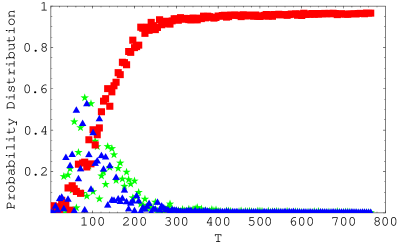
Figure 1. Corresponding equation $x-20=0$. See the main text for details.

4.2.2. Equation $xy+x+4y-11=0$

In this example, contrary to the one above, we fix the truncated size of our Fock space at all times to be $(m_{x},m_{y})=(9,9)$ so that the norm of the state vector is less than unity by an amount $\tilde{\epsilon}=10^{-2}$.

In Fig. 2, below $T\sim 1500$, the maximum probability components of $|\psi(T)\rangle$ are dominated by some states, denoted by (blue) star and (green) triangle symbols, none of which are the actual ground state. In fact, they are, respectively, the first degenerate excited states $|n_{x},n_{y}\rangle=|4,1\rangle$ and $|3,1\rangle$ of $H_{P}$.

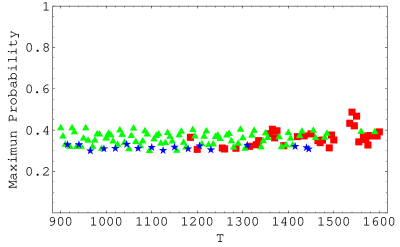
Figure 2. Corresponding equation $xy+x+4y-11=0$; with intermediate evolution time $T$. See the main text for details.

With $T$ increased in Fig. 3, one of the Fock states, namely $|1,2\rangle$ denoted by (red) boxes, has the measurement probability greater than ${1}/{2}$, which is our criterion for being identified as the ground state. From the ground state so identified we can infer that our Diophantine equation has a solution, which can be duly verified.

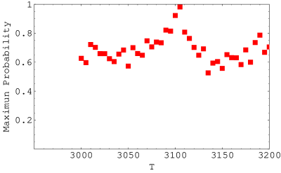
Figure 3. Corresponding equation $xy+x+4y-11=0$ as in Fig. 2 but with $T$ entering the quantum adiabatic regime.

4.2.3. Equation $x+20=0$

We consider this simple equation as an example which has no solution in the positive integers. The simulation parameters are as in the previous, except that the initial truncated size of our Fock space is up to $|n\rangle=8$ and is allowed to expand in time.

Below $T\sim 50$ in Fig. 4 none of the two components is greater than one-half, and in fact the first excited state, $|1\rangle$ denoted by (blue) triangles, clearly dominates in this regime. Eventually we enter the quantum adiabatic regime upon when the (red) boxes rise over the one-half mark; indeed it corresponds to the Fock state $|0\rangle$, which is the true ground state and which implies that our original Diophantine equation has no integer solution at all.

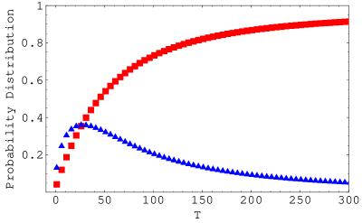
Figure 4. Corresponding equation $x+20=0$. See the main text for details.

5. On physical implementations

5.1. Misunderstandings and/or prejudices

Since the first announcement of an earlier version of the quantum adiabatic algorithm in 2001, there have been numerous discussions in private but only few postings have yet appeared in the public domain which are directly related to and/or built on the algorithm [52, 49, 47, 48, 50, 54], see also the Notes added at the end of this paper.

In this Subsection we will point out some of the misunderstandings, expressed either privately or publicly, that we know of which are directed towards the algorithm.

1. Our proposal is in contrast to the claim in [4] that quantum Turing machines compute exactly, albeit perhaps more efficiently, the same class of functions which can be computed by classical Turing machines. The quantum Turing machine approach is a direct generalisation of that of the classical Turing machines but with qubits and some universal set of one-qubit and two-qubit unitary gates to build up, step by step, dimensionally larger, but still dimensionally finite unitary operations. This universal set is chosen on its ability to evaluate any desirable classical logic function. Our approach, on the other hand, is already from the start based on infinite-dimension Hamiltonians acting on some Fock space and also based on the special properties and unique status of their ground states. These are the reasons behind the ability to compute, in a finite number of steps, what the dimensionally finite unitary operators of the standard quantum Turing computation cannot do in a finite number of steps.

   Indeed, several authors (including Nielsen [35] and Calude and Pavlov [6]) have also found no logical contradiction in applying the most general quantum mechanical principles (over and above those employed in the standard quantum computation) to the computation of the classical noncomputable, unless certain Hermitean operators cannot somehow be realised as observables or certain unitary processes cannot somehow be admitted as quantum dynamics. And up to now we have neither any evidence nor any principles that prohibit these kinds of observables and dynamics.

2. Recently there is a proof that QAC is equivalent to the more standard quantum computation [1]. That this equivalence generates no contradiction between the hypercomputability of QAC and the Turing computability of standard quantum computation can be seen from the facts that (i) such a proof of equivalence is only valid for finite Hilbert spaces; and (ii) the hypercomputability of QAC is also based on its probabilistically correct nature which escapes the jurisdiction of Cantor’s diagonal arguments as discussed in Subsection 3.7

3. In the early days there was a claim by Tsirelson that our proposed algorithm would not work [52]. We have immediately replied [22] and pointed out the fallacy of the criticism (but somehow the criticism is still propagating in some circle, where our reply is not acknowledged). It suffices to point out here that were Tsirelson correct then the quantum adiabatic theorem itself would have been wrong, not just our algorithm. But, of course, there is no basis to suspect the mathematically and physically proven QAT.

4. Our algorithm requires the ability to generate/simulate polynomials in the destruction and creation operators $a$ and $a\dagger$ (3.1) to arbitrarily finite orders. These can be simulated in quantum optics [31] with just mirrors, beam splitters, phase shifts, squeezing and Kerr non-linearity – despite the appearance of higher powers of the linear momentum operators  which has led some people to wrongly think that such polynomials could not be generated physically.

5. Others cling to the fact that Grover’s quantum search [21] of an unstructured database of size $M$ would need a number of computation steps of order $O(\sqrt{M})$ to claim that our algorithm would then need an infinite time to search the infinite underlying space. It suffices to note that our search is based on different principles than those of Grover’s. In fact, there do exist in the literature some other quantum search algorithms, for example [14], that are different to ours and Grover’s and yet whose complexity are not bounded by the size of the search database as O($\sqrt{M}$).

6. Yet others have erroneously based on a flawed application and interpretation of the energy-time uncertainty principle to claim that we could not measure the precise energy of the ground state of our algorithm in a finite time.

   • This is a flawed application of the uncertainty principle because our algorithm does not require measurement of arbitrarily small energy differences. As a matter of facts, the final energy spectrum of $H_{P}$ is integer-valued, and as such one only needs to distinguish energies that are separated by at least one integer unit, not by an arbitrarily small amount. Such measurement is allowed by the uncertainty principle and can be completed in a finite time when the energy uncertainties are sufficiently smaller than the energy unit by which the energy eigenstates are at least separated.

   • That this is a flawed interpretation of the uncertainty principle can be seen from the results [2, 3] that the energy can be measured in an arbitrarily short time for our algorithm through the instantaneous measurements of the (Fock) occupation numbers, one for each variables in the original Diophantine equation, of the final ground state. These measurements are compatible with the energy measurement because the final Hamiltonian $H_{P}$ commutes, by construction, with the Fock occupation number operators. And once obtained, these integer-valued occupation numbers can be simply substituted into the original Diophantine to reveal the lack or existence of integer solution for the equation, and also to evaluate the energy of the ground state. Thus the ground state energy need not be measured directly, even though it can be done with some care taken to calibrate the energy zero point.

7. This last point leads us to the question whether such integer-valued occupation numbers can be obtained for very large values if the universe is finite. The short answer to this question is obviously NO if the universe is in fact finite, see [28] in replying to [49]. But this could be a misleading question to be asked.

   Is the universe finite? We do not know for sure, but this is an important physics question and will surely be investigated and debated thoroughly in the years to come. But if it is then all computation, including Turing computation, must be limited, let alone any hypercomputation. Full stop. With finite physical resources, any Turing machine can physically compute only some finite number of the binary digits of any real number. For any number larger than this physical limit, only abstract mathematical representations can exist. In this way, we would have to conclude that $\pi$, for example, were Turing noncomputable too! Also, ‘most’ rational numbers would have been classified noncomputable! Clearly, this is too restrictive and not very useful a discussion of computable numbers. In fact, with such restriction, one would not need the concepts of effective computation and of recursive functions in general. Nor would one need the thesis of Church Turing at all – let alone hoping that the physical finiteness of the universe would support the thesis itself.

   In short, the physical finiteness of the universe should not impose any limitations on hypercomputation more than those which it would already impose on Turing computation since, in the end, all computation is physical. Because of this indiscrimination, it is logically inconsistent and simply wrong to use the finiteness arguments to rule out hypercomputation while still maintaining and defending the validity of Turing computation and the Church-Turing thesis. On the other hand, the physical finiteness should not and cannot stop us from investigating hypercomputation as it has not deterred us from studying Turing computation (or mathematics in general).

8. The physical finiteness of the universe would of course impose some upper limit on the number of dimensions one can physically realise. But as we know when in a Turing computation the end of a Turing tape has been reached and cannot be lengthened further due to lack of resources, we should also know when the upper dimensions of the computation Hilbert space have been physically arrived at. At that point, the computation would have to be abandoned before we could obtain the final result. At no time, however, the physical finiteness of the universe should lead us to the wrong computation result; it simply would not allow us to complete the computation for some group of Diophantine equations.

   All this depends on whether we could find a probability measure to quantify, for our final results, the uncertainty associated with a finite number of dimensions of the underlying Hilbert space. We hope to pursue this issue elsewhere.

9. What if quantum mechanics is wrong? A successful theory like quantum mechanics should not be considered wrong, it could only have a limited domain of validity, outside which another physical theory should take over. The question then is whether that validity domain is good enough for our proposed algorithm. The answer to this question is unknown at present and as long as quantum mechanics still proven to be consistently applicable to all phenomena, without any exception, that can be observed – as is the situation presently. The alternative to an exploration of a theory, including quantum mechanics, for fear that the theory might not be applicable is to do nothing meaningful.

5.2. Possible difficulties faced in a physical implementation

We could perhaps implement the algorithm, among other methods, with quantum optical apparatuses in which a beam of quantum light is the physical system on which final measurements are performed and the number of photons is the quantity measured. The Hamiltonians could then be physically simulated by various components of mirrors, beam splitters, Kerr-nonlinear media (with appropriate efficiency), squeezing [31, 27, 24]. We should differentiate the relative concepts of energy involved in this case; a final beam state having one single photon, say, could correspond to a higher energy eigenstate of $H_{P}$ than that of a state having more photons! Only in the final act of measuring photon numbers, the more-photon state would transfer more energy in the measuring device than the less-photon state.

The road leading to such a realisation, even if it is not explicitly prohibited by some known or to-be-found physical principles, is of course not without problems.

1. A possible problem is that the Hamiltonians which we need to be simulated in the optical apparatuses are only effective Hamiltonians in that their descriptions are only valid for certain range of number of photons. When there are too many photons, a mirror, for example, may respond in a different way from when only a few photons impinge on it, or the mirror may simply melt down. That is, other more fundamental processes/Hamiltonians different than the desirable effective Hamiltonians would take over beyond certain limit in the photon numbers.

   This situation is not unlike that of the required unboundedness of the Turing tape. In practice, we can only have a finite Turing tape/memory/register; and when the register is overflowed we would need to extend it. Similar to this, we would have to be content with a finite range of applicability for our simulated Hamiltonians. But we should also know the limitation of this applicability range and be able to tell when in a quantum computation an overflow has occurred – that is, when the range of validity is breached. We could then use new materials with extended range of (photon number) applicability.

   On the other hand, however, one should note that infinite dimensions are common and essential in Quantum Mechanics. For example, it is well known that no finite-dimensional matrices can possibly satisfy the commutator 

   $$x\,p-p\,x=i\hbar\,{\bf 1}.$$

2. The ability to control or suppress environmental effects is also another crucial requirement for the implementation of our quantum algorithm. The coupling with the environment causes some fluctuations in the energy levels. Ideally, the size of these fluctuations should be controlled and reduced to a degree that is smaller than the size of the smallest energy gap such as not to cause transitions out of the adiabatic process. This may present a difficulty for our algorithm, but maybe one of technical nature rather than of principle. Even though these fluctuations in the energy levels are ever present and cannot be reduced to zero, there is no physical principle, and hence no physical reason, why their sizes cannot be reduced to a size smaller than some required scale.

   More specifically are fluctuations in the values of the (integer) coefficients of the Diophantine equations being implemented in the Hamiltonian $H_{P}$ . Those fluctuations will result in a wrong representation of the Diophantine equation and thus in erroneous outcomes. If the fluctuations are systematic then the Diophantine equation cannot be represented correctly at all, and we then cannot do anything much. The case we wish to investigate elsewhere is the stochastic but non-biased fluctuations, so that the time averages of the coefficients in $H_{P}$ have the correct values. Of particular interest is how the ground state and its measurement probability would be affected by and would scale with the sizes of such fluctuations in the coefficients, which could be reduced arbitrarily even though non-vanishing.

3. Recently we have found an interesting and intimate connection between our algorithm and the so called Mott insulator - superfluid quantum phase transitions, which have recently been experimentally confirmed [20]. Quantum phase transitions [45] are purely due to quantum fluctuations, unlike other types of phase transitions, such as liquid-vapour transitions, which are due entirely to the thermal fluctuations. In principle, quantum fluctuations can thus take place even at zero absolute temperature. This connection thus irrefutably demonstrates the possibility of physical implementations for our algorithm, at least for certain classes of Diophantine equations. The details of the connection will be published elsewhere. It suffices to mention here that such a connection is possible because the underlying process for quantum phase transitions is also the quantum adiabatic process that governs the dynamics of the quantum adiabatic algorithm.

6. Concluding remarks

In this paper we have given an overview of the working of an adiabatic quantum algorithm for Hilbert’s tenth problem. Numerical simulations for some simple Diophantine equations have also been reported together with an explanation how we should cope with the required dimensionally-unbounded Hilbert space.

Our algorithm is not just another quantum algorithm in the sense that it can substantially speed up what can be computed on classical computers, but it presents a new paradigm of computation. It is arguably in the area of hypercomputation, the kind of computability beyond that delimited by the Church-Turing thesis. This is due to the facts that: (i) it belongs to the class of probabilistically correct algorithms which are not subject to Cantor’s diagonal arguments as we have pointed out above in Subsection 3.7; and (ii) it is based on the most general principles of quantum mechanics which are definitely and irrefutably non-recursive as can be seen through the class of Schrödinger equations (4.1) and through their ability to generate truly random numbers.

The fact that our algorithm is “only” probabilistically correct can be understood as a necessity and a consistency condition when the outcomes of such an algorithm cannot, in principle, be verified by any other means. The algorithm gives the $k$-tuple at which the square of a Diophantine polynomial assumes it smallest value. While the existence of a solution can be verified by a simple substitution, the indication of no solution cannot be verified by any other finite recursive means at all – thus the need of some probability measure to quantify the accuracy of the derived conclusion. However, it is important and useful that this probability is not only known but can also be predetermined with an arbitrary value in advance.

The algorithm is based on the quantum adiabatic theorem, which asserts that a particular eigenstate of a final-time Hamiltonian, even in dimensionally infinite spaces, could be found mathematically and/or physically in a finite time. This is a remarkable property, which is enabled by quantum interference and quantum tunnelling with complex-valued probability amplitudes, and allows us to find a needle in an infinite haystack, in principle! Such a property is clearly not available for recursive search in an unstructured infinite space, which, in general, cannot possibly be completed in a finite time, in contrast to the quantum scenario.

This is what we mean by “an infinite search in a finite time”: Of course, the spread of a quantum wavefunction in an adiabatic process for a finite time can only cover essentially a finite domain of the underlying infinite space, but the finite domain so covered is the relevant domain, as guaranteed by the quantum adiabatic theorem, for a successful location of the global minimum (which is the search objective) in a finite time – whence the locating result is necessarily subject to some probability of error which can nevertheless be arbitrarily reduced.

That is the point. Just like water in a porous landscape always accumulates at the lowest point after some finite time even when the size of the landscape is infinite (since the water need not explore the whole space), a quantum state (starting from appropriate initial conditions) could also accumulate (adiabatically and probabilistically) at the global minimum (of some bounded-from-below Hamiltonian) – even in an infinite Hilbert space – given sufficient but finite time for it to perform its quantum tunneling instinct.

The failure of Cantor’s diagonal arguments to rule out the use of probabilistic procedure for hypercomputation leaves open the possibility that we could employ a single and universal, albeit probabilistically correct, algorithm to compute some recursively non-computable, provided we are prepared to be wrong – with an error probability that can be made arbitrarily small. This fact was recognised in one form or another by Gödel and Turing themselves a long time ago (see [30] for some discussions and quotations). And we would like to think that that probabilistic hypercomputation possibility is the quantum adiabatic algorithm we have proposed for Hilbert’s tenth problem and its associated class of problems. Perhaps this hypercomputability of quantum adiabatic processes could be generalised further to a wider class of finitely refutable problems?

Elsewhere, in the earlier stage of development of the algorithm, I thought and accordingly stated that the ability to implement dimensionally infinite Hamiltonians was absolutely necessary [23]. While that ability is sufficient and certainly of great help for our hypercomputational algorithm and others [54], I am now of the opinion that it would not be quite absolutely necessary if we could quantify the uncertainties associated with truncated Hilbert spaces by some error probabilities for the outcomes. We will pursue this issue elsewhere.

Intimately linked with this computability study are the physical phenomena of quantum phase transitions (QPT). The fact that certain QPT is the physical realisation of instances of our algorithms for Hilbert’s tenth problem is surprising, extraordinary and of great consequence. It does not only illustrate that certain instances of the algorithm are physically implementeble but also raises the prospect of a much deeper connection between QAC, quantum computability and QPT.

These studies into the limit of mathematics and generalised noncomputability and undecidability set the bounds for computation carried out by mechanical (including quantum mechanical) processes, and in so doing help us to understand much better what can be so computed. It should enable us to algorithmically resolve many important and interesting mathematical problems. It would further contribute to other fields of philosophy and artificial intelligence – in the debate, for example, whether human minds can be simulated (or even be replaced) by machines and computers.

Notes added

During the course of writing this paper I have learned about Martin Davis’ comments [17] about my not responding to Andrew Hodges’ critique of the algorithm as posted on FOM (a forum on Foundation of Mathematics moderated by Davis). In fact, we have had not only with Hodges but also with other people quite a few discussions, for which I am very grateful. However, after some initial exchanges, I have explicitly stated on FOM to the effect that I thought that the forum, while useful for clearing up some misunderstandings, was neither the appropriate medium nor a primary publication place for settling deep disagreements. I have also proposed to these people that their opposing arguments should be published for the record. (And this should also apply to “the leading experts in quantum computation” who have advised Davis against my proposed algorithm, as I have never seen their arguments in print – except those in [52], [49], respectively to which I have already replied in [22], [28].) I myself have, for the record, addressed above in this paper and also elsewhere [30] some of the points (that I know of) raised by Hodges and others about the algorithm.

References

- [1] D. Aharonov, W. van Dam, J. Kempe, Z. Landau, S. Lloyd, and O. Regev. Adiabatic computation is equivalent to standard quantum computation. ArXiv:quant-ph/0405098, 2004.
- [2] Y. Aharonov and D. Bohm. Time in the quantum theory and the uncertainty relation for time and energy. Phys. Rev., 122:1649–1658, 1961.
- [3] Y. Aharonov, S. Massar, and S. Popescu. Measuring energies, estimating Hamiltonians, and the time-energy uncertainty relation. Phys. Rev. A, 66:052107, 2002.
- [4] E. Bernstein and U. Vazirani. Quantum complexity theory. SIAM J. Comp., 26:1411, 1997.
- [5] C.S. Calude. Information and Randomness: An Algorithmic Perspective. Springer-Verlag, Berlin Heidelberg, 2nd edition, 2002.
- [6] C.S. Calude and B. Pavlov. Coins, quantum measurements, and turing’s barrier. Quantum Information Processing, 1:107–127, 2002.
- [7] J.L. Casti. Mathematical Mountaintops: The Five Most Famous Problems of All Time. Oxford University Press, New York, 2001.
- [8] J.L. Casti and W. DePauli. Gödel: A Life of Logic. Perseus Publishing, Cambridge, Massachusetts, 2000.
- [9] G.J. Chaitin. Algorithmic Information Theory. Cambridge University Press, Cambridge, 1987.
- [10] G.J. Chaitin. Meta Math! The Quest for . Pantheon Books, New York, 2005.
- [11] A.M. Childs, E. Farhi, and J. Preskill. Robustness of adiabatic quantum computation. Phys. Rev. A, 65:012322, 2002.
- [12] J. Copeland. Hypercomputation. Minds and Machines, 12:461–502, 2002.
- [13] P. Cotogno. Hypercomputation and the physical Church-Turing thesis. Brit. J. Phil. Sci., 54:181–223, 2003.
- [14] S. Das, R. Kobes, and G. Kunstatter. Energy and efficiency of adiabatic quantum search algorithms. J. Phys. A, 36:2839–46, 2003.
- [15] M. Davis. Engines of Logic: Mathematicians and the Origin of the Computer. W.W. Norton, New York, 2001.
- [16] M. Davis. The myth of hypercomputation. In C. Teuscher, editor, Alan Turing: Life and Legacy of a Great Thinker, pages 195–212. Springer, Berlin, 2004.
- [17] M. Davis. Why there is no such discipline as hypercomputation. This issue, 2005.
- [18] K. de Leeuw, E.F. Moore, C.E. Shannon, and N. Shapiro. Number 34 in Automata Studies Annals of Mathematics Studies. Princeton University Press, Princeton, 1956.
- [19] E. Farhi, J. Goldstone, S. Gutmann, and M. Sipser. Quantum computation by adiabatic evolution. ArXiv:quant-ph/0001106, 2000.
- [20] M. Greiner, O. Mandel, T.W. Hänsch, and I. Bloch. Collapse and revival of the matter wave field of a Bose-Einstein condensate. Nature, 419:51–54, 2002.
- [21] L.K. Grover. Quantum mechanics helps in searching for a needle in a haystack. Phys. Rev. Lett., 79:325–328, 1997.
- [22] T.D. Kieu. Reply to ‘The quantum algorithm of Kieu does not solve the Hilbert’s tenth problem’. ArXiv:quant-ph/0111020, 2001.
- [23] T.D. Kieu. Quantum hypercomputation. Minds and Machines, 12:541–561, 2002.
- [24] T.D. Kieu. Computing the non-computable. Contemporary Physics, 44:51–77, 2003.
- [25] T.D. Kieu. Numerical simulations of a quantum algorithm for Hilbert’s tenth problem. In Eric Donkor, Andrew R. Pirich, and Howard E. Brandt, editors, Proceedings of SPIE Vol. 5105 Quantum Information and Computation, pages 89–95. SPIE, Bellingham, WA, 2003.
- [26] T.D. Kieu. Quantum adiabatic algorithm for Hilbert’s tenth problem: I. The algorithm. ArXiv:quant-ph/0310052, 2003.
- [27] T.D. Kieu. Quantum algorithms for Hilbert’s tenth problem. Int. J. Theor. Phys., 42:1451–1468, 2003.
- [28] T.D. Kieu. Finiteness of the universe and computation beyond Turing computability. ArXiv:quant-ph/0403045, 2004.
- [29] T.D. Kieu. A reformulation of Hilbert’s tenth problem through quantum mechanics. Proc. Roy. Soc., A 460:1535–1545, 2004.
- [30] T.D. Kieu. An anatomy of a quantum adiabatic algorithm that transcends the Turing computability. Int. J. Quantum Info., 3:177–182, 2005.
- [31] S. Lloyd and S. Braunstein. Quantum computation over continuous variables. Phys. Rev. Lett., 82:1784, 1999.
- [32] Y.V. Matiyasevich. Hilbert’s Tenth Problem. MIT Press, Cambridge, Massachussetts, 1993.
- [33] Y.V. Matiyasevich. Diophantine flavour of Kolmogorov complexity. http://at.yorku.ca/cgi-bin/amca/cani-11, 2004.
- [34] A. Messiah. Quantum Mechanics. Dover, New York, 1999.
- [35] M.A. Nielsen. Computable functions, quantum measurements, and quantum dynamics. Phys. Rev. Lett., 79:2915–8, 1997.
- [36] M.A. Nielsen and I.L. Chuang. Quantum Computation and Quantum Information. Cambridge University Press, Cambridge, 2000.
- [37] T. Ord. Hypercomputation: Computing more than the Turing machine. Honours Thesis, University of Melbourne, Melbourne, Australia, September 2002. Also available at ArXiv:math.LO/0209332, 2002.
- [38] T. Ord. Hypercomputation: computing more than the Turing Machine. This issue, 2005.
- [39] T. Ord and T.D. Kieu. On the existence of a new family of Diophantine equations for . Fundmenta Informaticae, 56:273–84, 2003.
- [40] T. Ord and T.D. Kieu. Using biased coins as oracles. Arxiv:cs.OH/0401019, 2004.
- [41] T. Ord and T.D. Kieu. The diagonal method and hypercomputation. Brit. J. Phil. Sci., 56:147–156, 2005.
- [42] M.B. Pour-El and J.I. Richards. Computability in Analysis and Physics. Sringer-Verlag, Berlin-Heidelberg, 1989.
- [43] M. Reed and B. Simon. Methods of Modern Mathematical Physics: IV Analysis of Operators. Academic Press, San Diego, 1978.
- [44] Y.A. Rozanov. Probability Theory: A Concise Course. Dover, New York, 1977.
- [45] S. Sachdev. Quantum Phase Transitions. Cambridge University Press, Cambridge, 1999.
- [46] E.S. Santos. Computability by probabilistic Turing machines. Trans. Am. Math. Soc., 159:165–184, 1971.
- [47] A. Sicard, J. Ospina, and M. Vélez. Numerical simulations of a possible hypercomputational quantum algorithm. In B. Ribeiro et al., editors, Proceedings of the International Conference on Adaptive and Natural Computing Algorithms. Springer Wien NewYork, 2005.
- [48] A. Sicard, M. Vélez, and J. Ospina. Hypercomputation based on quantum computing. ArXiv:quant-ph/0406137, 2004.
- [49] R. Srikanth. Computable functions, the Church-Turing Thesis and the quantum measurement problem. ArXiv:quant-ph/0402128, 2004.
- [50] R. Srinivasan and H.P. Raghunandan. On the existence of truly autonomic computing systems and the link with quantum computing. ArXiv:cs.LO/0411094, 2004.
- [51] M. Stannett. Hypercomputation is experimentally irrefutable. Sheffield University Department of Computer Science Report TR CS-01-04, 2001.
- [52] B. Tsirelson. The quantum algorithm of Kieu does not solve the Hilbert’s tenth problem. ArXiv:quant-ph/0111009, 2001.
- [53] P.D. Welch. On the possibility, or otherwise, of hypercomputation. Brit. J. Phil. Sci., 55:739–746, 2004.
- [54] M. Ziegler. Does quantum mechanics allow for infinite parallelism? ArXiv:quant-ph/0410141, 2004.