Theory of slow-light solitons

Abstract

In the framework of the nonlinear $\Lambda$-model we investigate propagation of solitons in atomic vapors and Bose-Einstein condensates. We show how the complicated nonlinear interplay between fast solitons and slow-light solitons in the $\Lambda$-type media points to the possibility to create optical gates and, thus, to control the optical transparency of the $\Lambda$-type media. We provide an exact analytic description of decelerating, stopping and re-accelerating of slow-light solitons in atomic media in the nonadiabatic regime. Dynamical control over slow-light solitons is realized via a controlling field generated by an auxiliary laser. For a rather general time dependence of the field; we find the dynamics of the slow-light soliton inside the medium. We provide an analytical description for the nonlinear dependence of the velocity of the signal on the controlling field. If the background field is turned off at some moment of time, the signal stops. We find the location and shape of the spatially localized memory bit imprinted into the medium. We discuss physically interesting features of our solution, which are in a good agreement with recent experiments.

I Introduction.

Recent progress in experimental techniques for the coherent control of light-matter interaction opens many opportunities for interesting practical applications. The experiments are carried out on various types of materials such as cold sodium atoms Hau et al. (1999); Liu et al. (2001), rubidium atom vapors Phillips et al. (2001); Bajcsy et al. (2003); Braje et al. (2003); Mikhailov et al. (2004), solids Turukhin et al. (2002); Bigelow et al. (2003), photonic crystals Soljacic and Joannopoulos (2004). These experiments are based on the control over the absorption properties of the medium and study slow light and superluminal light effects. The control can be realized in the regime of electromagnetically induced transparency (EIT), by the coherent population oscillations or other induced transparency techniques. The use of each different materials brings specific advantages important for the practical realization of the effects. For instance, the cold atoms have negligible Doppler broadening and small collision rates, which increases ground-state coherence time. The experiments on rubidium vapors are carried at room temperatures and this does not require application of complicated cooling methods. The solids are obviously one of the strongest candidates for realization of long-living optical memory. Photonic crystals provide a broad range of paths to guide and manipulate the slow light. The interest in the physics of light propagation in atomic vapors and Bose-Einstein condensates (BEC) is strongly motivated by the success of research on storage and retrieval of optical information in these media Hau et al. (1999); Liu et al. (2001); Phillips et al. (2001); Kocharovskaya et al. (2001); Bajcsy et al. (2003); Dutton and Hau (2004).

Even though the linear approach to describing these effects based on the theory of electromagnetically induced transparency (EIT) Harris (1997) is developed in detail Lukin (2003), modern experiments require more complete nonlinear descriptions Dutton and Hau (2004). The linear theory of EIT assumes the probe field to be much weaker than the controlling field. To allow significant changes in the initial atomic state due to interaction with the optical pulse, here we go beyond the limits of linear theory. In the adiabatic regime, when the fields change in time very slowly, approximate analytical solutions Grobe et al. (1994); Eberly (1995) and self-consistent solutions Andreev (1998) were found and later applied in the study of processes of storage and retrieval Dey and Agarwal (2003). Different EIT and self-induced transparency solitons of nonlinear regime were classified and numerically studied for their stability Kozlov and Eberly (2000). As it was demonstrated by Dutton and coauthors Dutton et al. (2001) strong nonlinearity can result in interesting new phenomena. Recent experiments and numerical studies Matsko et al. (2001); Dutton and Hau (2004) have shown that the adiabatic condition can be relaxed allowing for much more efficient control over the storage and retrieval of optical information.

In this paper we study the interaction of light with a gaseous active medium whose working energy levels are well approximated by the $\Lambda$-scheme. Our theoretical model is a very close prototype for a gas of sodium atoms, whose interaction with the light is approximated by the structure of levels of the $\Lambda$-type. The structure of levels is given in Fig. 1, where two hyperfine sub-levels of sodium state $3^{2}S_{1/2}$ with $F=1,F=2$ are associated with $|2\rangle$ and $|1\rangle$ states, correspondingly Hau et al. (1999). The excited state $|3\rangle$ corresponds to the hyperfine sub-level of the term $3^{2}P_{3/2}$ with $F=2$. We consider the case when the atoms are cooled down to microkelvin temperatures in order to suppress the Doppler shift and increase the coherence life-time for the ground levels. The atomic coherence life-time in sodium atoms at a temperature of $0.9{\mu}$K is of the order 0.9 ms Liu et al. (2001). Typically, in the experiments the pulses have length of microseconds, which is much shorter than the coherence life-time and longer than the optical relaxation time of $16.3ns$.

The gas cell is illuminated by two circularly polarized optical beams co-propagating in the z-direction. One beam, denoted as channel $a$, is a $\sigma^{-}$-polarized field, and the other, denoted as $b$, is a $\sigma^{+}$-polarized field. The corresponding fields are presented within the slow-light varying amplitude and phase approximation (SVEPA) as

$$\vec{E}=\vec{e}_{a}\,\mathcal{E}_{a}e^{i(k_{a}z-\omega_{a}t)}+\vec{e}_{b}\,\mathcal{E}_{b}e^{i(k_{b}z-\omega_{b}t)}+c.c.$$ (1)

Here, $k_{a,b}$ are the wave numbers, while the vectors $\vec{e}_{a},\vec{e}_{b}$ describe polarizations of the fields. It is convenient to introduce two corresponding Rabi frequencies:

$$\Omega_{a}=\frac{2\mu_{a}\mathcal{E}_{a}}{\hbar},\Omega_{b}=\frac{2\mu_{b}\mathcal{E}_{b}}{\hbar},$$ (2)

where $\mu_{a,b}$ are dipole moments of quantum transitions in the channels $a$ and $b$.

In the interaction picture and within the SVEPA, the Hamiltonian $H_{\Lambda}=H_{0}+H_{I}$ describing the interaction of a three-level atom with the fields is defined as follows:

$$H_{0}=-\frac{\Delta}{2}D,\;H_{I}=-\frac{1}{2}\left({\Omega_{a}|3\rangle\langle 1|+\Omega_{b}|3\rangle\langle 2|}\right)+h.c.,$$ (3)

where

$$D=\left(\begin{array}[]{ccc}1&0&0\\ 0&1&0\\ 0&0&-1\\ \end{array}\right).$$

Here $\Delta$ is the variable detuning from the resonance and we set $\hbar=1$.

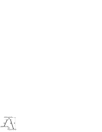
Figure 1: The $\Lambda$-scheme for working energy levels of sodium atoms. The parameters of the scheme are the following: $\omega_{12}/(2\pi)=1772\mathrm{MHz}$, $\omega/(2\pi)=5.1\cdot 10^{14}\mathrm{Hz}$ ($\lambda=589\mathrm{nm}$), and $\Delta$ is the variable detuning from the resonance.

The dynamics of the fields is described by the Maxwell equations

$$(\partial_{t}^{2}-c^{2}\partial_{z}^{2})\Omega_{a}e^{i(k_{a}z-\omega_{a}t)}=-\frac{2\nu_{a}}{\omega_{a}}\partial_{t}^{2}\left({\rho_{31}e^{i(k_{a}z-\omega_{a}t)}}\right),$$

$$(\partial_{t}^{2}-c^{2}\partial_{z}^{2})\Omega_{b}e^{i(k_{b}z-\omega_{b}t)}=-\frac{2\nu_{b}}{\omega_{b}}\partial_{t}^{2}\left({\rho_{32}e^{i(k_{b}z-\omega_{b}t)}}\right),$$

where $\nu_{a}=(n_{A}|\mu_{a}|^{2}\omega_{a})/\epsilon_{0}$, $\nu_{b}=(n_{A}|\mu_{b}|^{2}\omega_{b})/\epsilon_{0}$, $n_{A}$ is the density of atoms, and $\epsilon_{0}$ is the vacuum susceptibility. Here $\rho$ is the density matrix in the interaction representation. For typical experimental situations the coupling constants $\nu_{a,b}$ are almost the same. Therefore we assume that $\nu_{a}=\nu_{b}=\nu_{0}$. Hence, within the SVEPA the wave equations are reduced to the first order PDEs:

$$\partial_{\zeta}\Omega_{a}=i\nu_{0}\,\rho_{31},\;\partial_{\zeta}\Omega_{b}=i\nu_{0}\,\rho_{32}.$$ (4)

Equations Eqs.(4) can be rewritten in a matrix form as

$$\partial_{\zeta}H_{I}=i\frac{\nu_{0}}{4}\left[{D,\rho}\right],$$ (5)

In the new variables the Liouville equation takes the form

$$\partial_{\tau}\rho=i\left[{\frac{\Delta}{2}D-H_{I},\rho}\right].$$ (6)

Here $\zeta=z/c$, $\tau=t-z/c$. To make parameters dimensionless, we measure the time in units of optical pulse length $t_{p}=1\mu s$ typical for the experiments on the slow-light phenomena Bajcsy et al. (2003). We also normalize the spatial coordinate to the spatial length of the pulse slowed down in the medium, i.e. $l_{p}=v_{g}t_{p}\approx c\frac{\Omega_{0}^{2}}{2\nu_{0}}\;t_{p}$. Here $\Omega_{0}$ is a typical magnitude of the controlling field required in EIT experiments. We assume this field to be of order a few megahertz. We choose $\Omega_{0}=3$ as a representative value. This corresponds to a group velocity of several meters per second, depending on the density of the atoms. We take the group velocity to be $10^{-7}c$, so the pulse spatial length is $30\mu m$, and $\zeta$ is normalized to $10^{-13}s$. Then, in the dimensionless units, the coupling constant $\nu_{0}=\frac{\Omega_{0}^{2}}{2}=4.5$. The retarded time $\tau$ is measured in microseconds and the Rabi frequencies are normalized to $\mathrm{MH}z$.

The system of equations Eqs.(5),(6) is exactly solvable in the framework of the inverse scattering (IS) method Faddeev and Takhtadjan (1987); Park and Shin (1998); Byrne et al. (2003); Rybin and Vadeiko (2004). This means that the system of equations Eqs.(5),(6) constitutes a compatibility condition for a certain linear system, namely

$$\partial_{\tau}\Phi=U(\lambda)\,\Phi=\frac{i}{2}\lambda D\,\Phi\,-iH_{I}\,\Phi,$$ (7)

$$\partial_{\zeta}\Phi=V(\lambda)\,\Phi=\frac{i}{2}\frac{\nu_{0}\rho}{\lambda-\Delta}\,\Phi\,.$$ (8)

Here, $\lambda\in{\mathbb{C}}$ is the spectral parameter. The comparison $\Phi_{\tau\zeta}$ against $\Phi_{\zeta\tau}$ leads to the zero-curvature condition Faddeev and Takhtadjan (1987) $U_{\zeta}(\lambda)-V_{\tau}(\lambda)+\left[U(\lambda),V(\lambda)\right]=0$, which holds identically with respect to the linearly independent terms in $\lambda$. It is straightforward to check that the resulting conditions coincide with the nonlinear equations Eqs.(5),(6). At this point it is worth discussing the initial and boundary conditions underlying the physical problem in question. We consider a semi-infinite $\zeta\geq 0$ active medium with a pulse of light incident at the point $\zeta=0$ (initial condition). This means that the evolution is considered with respect to the space variable $\zeta$, while the boundary conditions should be specified with respect to the variable $\tau$. In our case we use as the asymptotic boundary conditions the asymptotic values of the density matrix at $\tau\to\pm\infty$. To solve the nonlinear dynamics as described by equations Eqs.(5),(6), the IS method considers the scattering problem for the linear system Eq.(7), while the auxiliary linear system Eq.(8) describes the evolution of the scattering data. The purpose of this work is, in particular, to study an essentially nonlinear interplay of the fields in both the channels. This goal leads to considering for equation Eq.(7) the scattering problem of finite density type (cf. Faddeev and Takhtadjan (1987) and references therein), i.e. $\Omega_{a,b}\to\Omega_{a,b}^{\pm}$ as $\tau\to\pm\infty$. For an account of other results for the $\Lambda$-system accessible through the IS method see, for example, references Hioe and Grobe (1994); Grobe et al. (1994); Park and Shin (1998); Byrne et al. (2003). In this work we choose to use an algebraic version of the IS method, i.e. the Darboux-Bäcklund (DB) transformations. The DB method does not require a full investigation of the initial value problem and merely allows mounting of a soliton on a chosen background. The resulting solution is, of course, consistent with the underlying initial value problem. We use Darboux-Bäcklund transformations, in the spirit of Rybin et al. (1988); Rybin (1991); Rybin and Timonen (1993); Matveev and Salle (1991), up to certain modifications.

In the physical case considered in this report, the system is assumed to be initially in a stationary state described by the following background solution:

$$\Omega_{a}=0,\;\Omega_{b}=\Omega(\tau),\;\rho=|\psi_{at}\rangle\langle\psi_{at}|=|1\rangle\langle 1|.$$ (9)

Notice that the state $|1\rangle$ is a dark-state for the controlling field $\Omega(\tau)$. This means that the atoms do not interact with the field $\Omega(\tau)$ created by the auxiliary laser. The configuration Eq.(9) above corresponds to a typical experimental setup (see e.g. Hau et al. (1999); Liu et al. (2001); Bajcsy et al. (2003)). The function $\Omega(\tau)$ models the controlling field, which governs the dynamics of the system. The time dependence of this function can result from modulation of the intensity of the auxiliary laser. In general, $\Omega(\tau)$ can also depend on the spatial variable $\zeta$. However, we do not specify such dependence explicitly in the formalism below except for a simple case of linear phase shift, which is discussed in section III.

The paper is organized as follows. In the next section we describe the Darboux-Bäcklund transformation for the $\Lambda$-system. In section III we describe the mechanism of a transparency gate for the slow-light soliton. In section IV we discuss an exactly solvable example of manipulation of slow-light solitons, while section V considers a similar problem for the case of a fairly arbitrary controlling field. Section VI is devoted to conclusions and discussion.

II Darboux-Bäcklund transformation for the $\Lambda$-system

In this section we describe the Darboux-Bäcklund (DB) transformation for the $\Lambda$-system. First we reformulate the linear system Eqs.(7),(8) in the matrix form, viz.

$$\partial_{\tau}\Psi = \frac{i}{2}D\,\Psi\,{\cal L}-iH_{I}\,\Psi,$$ (10)

$$\partial_{\zeta}\Psi = \frac{i\nu_{0}}{2}{\rho}\,\Psi\,{\cal P}.$$ (11)

Here $\Psi$ is a matrix consisting of three linearly independent solutions of the linear system Eqs.(7),(8) corresponding to three (not necessarily different) values of the spectral parameter $\lambda$, i.e. $\lambda^{\prime},\lambda^{\prime\prime},\lambda^{\prime\prime\prime}$. The matrix spectral parameters ${\cal L}$ is defined as

$${\cal L}=\left(\begin{array}[]{ccc}\lambda^{\prime}&0&0\\ 0&\lambda^{\prime\prime}&0\\ 0&0&\lambda^{\prime\prime\prime}\\ \end{array}\right),$$

while ${\cal P}^{-1}={\cal L}-\Delta\cdot I$.

The $N$-fold ($N\geq 1$) Darboux-Bäcklund transformation can be formulated as

$$\Psi[N]=\sum\limits_{n=0}^{N}(-1)^{n+1}\,\Xi_{N-n}(\Delta)\Psi\,{\cal P}^{-n},\quad\Xi_{0}=I.$$ (12)

It is clear that the linear system Eqs.(10),(11) is covariant with respect to this transformation provided that for $0\leq n\leq N$ the following Darboux-Bäcklund dressing transformations are satisfied

$$H_{I}[N]\,\Xi_{N-n}(\Delta)=\Xi_{N-n}(\Delta)H_{I}+i\partial_{\tau}\Xi_{N-n}(\Delta)$$

$$-\frac{1}{2}\left[{D,\left({\Xi_{N-n+1}(\Delta)-\Delta\,\Xi_{N-n}(\Delta)}\right)}\right],$$ (13)

$$\rho[N]\,\Xi_{N-n}(\Delta)=\Xi_{N-n}(\Delta)\,\rho+\frac{2i}{\nu_{0}}\partial_{\zeta}\Xi_{N-n+1}(\Delta),\quad$$ (14)

together with the convention $\Xi_{N+1}(\Delta)\equiv\Xi_{0}(\Delta)=I$. The meaning of Eqs.(13),(14) is that they connect the ”seed” solutions $H_{I},\rho$ of the nonlinear system with the dressed ($N$-soliton) solutions $H_{I}[N],\rho[N]$. To derive the matrices $\left\{\Xi_{k}\right\}_{k=1}^{N}$, we specify a set of solutions $\left\{\Psi_{k}\right\}_{k=1}^{N}$ corresponding to certain fixed values of the matrix spectral parameter ${\cal L}$, i.e. $\left\{{\cal L}_{k}\right\}_{k=1}^{N}$, where

$${\cal L}_{k}=\left(\begin{array}[]{ccc}\lambda_{k-1}^{*}&0&0\\ 0&\lambda_{k-1}^{*}&0\\ 0&0&\lambda_{k-1}\\ \end{array}\right),\;{\cal P}_{k}^{-1}={\cal L}_{k}-\Delta\cdot I\,.$$

We then demand

$$\sum\limits_{n=0}^{N}(-1)^{n+1}\Xi_{N-n}(\Delta)\Psi_{k}\,{\cal P}_{k}^{-n}=0,\quad k=1,\ldots,N.$$ (15)

This linear system allows the dressing matrices $\left\{\Xi_{k}(\Delta)\right\}_{k=1}^{N}$ to be obtained through Cramer’s rule. It can be shown that solutions of Eq.(15) satisfy the relations Eqs.(13),(14).

Since in what follows we only discuss the case $N=1$ for convenience, we changed notations as follows $H_{I}[1]\to\tilde{H}_{I}$, $\rho[1]\to\tilde{\rho}$, $\Xi_{1}(\Delta)\to\Xi(\Delta)$. Then the dressing formulae Eqs.(12),(13),(14) reduce to

$$\tilde{H}_{I}=H_{I}-\frac{1}{2}\left[{D,\Xi(0)}\right],\;\tilde{\rho}=\Xi(\Delta)\,\rho\,\Xi^{-1}(\Delta)$$ (16)

$$\tilde{\Psi}=\Psi\,{\cal P}^{-1}-\Xi(\Delta)\Psi,$$ (17)

while from the linear system Eq.(15) we obtain

$$\Xi(\Delta)=\Psi_{1}({\cal L}_{1}-\Delta\cdot I)\Psi_{1}^{-1},$$ (18)

As was explained above, the matrix $\Psi_{1}$ is a specification of $\Psi$ corresponding to a particular value of the matrix spectral parameter:

$${\cal L}_{1}=\left(\begin{array}[]{ccc}\lambda_{0}^{*}&0&0\\ 0&\lambda_{0}^{*}&0\\ 0&0&\lambda_{0}\\ \end{array}\right).$$

We denote as $\Phi_{0}$ the fundamental matrix of solutions for the linear system Eqs.(7),(8) for $\lambda=\lambda_{0}$. It can be shown that for the value of the spectral parameter $\lambda=\lambda_{0}^{*}$ the fundamental matrix is $\bar{\Phi}_{0}\equiv(\Phi_{0}^{-1})^{\dagger}$. Since the subspace of solutions corresponding to $\lambda_{0}^{*}$ is two dimensional, the matrix $\Psi_{1}$ is constructed as follows. The vector $\Psi_{1}^{(3)}=c_{1}\Phi_{0}^{(1)}+c_{2}\Phi_{0}^{(2)}+c_{3}\Phi_{0}^{(3)}$ is a general solution of the linear problem with $\lambda=\lambda_{0}$. Here upper index in the brackets $i=1,2,3$ denotes a vector-column. To satisfy the structure of the operator $\Xi$ Eq.(17) we require that $(\Psi_{1}^{(3)},\Psi_{1}^{(1,2)})=0$, where $(\cdot,\cdot)$ denotes a scalar product of two vectors in 3D complex vector space, and the vectors $\Psi_{1}^{(1,2)}$ correspond to $\lambda=\lambda_{0}^{*}$. Due to the definition $(\bar{\Phi}_{0}^{(i)},\Phi_{0}^{(j)})=\delta_{i,j}$.

We can easily find two appropriate orthogonal vectors $\Psi_{1}^{(1,2)}$:

$$\Psi_{1}^{(1)}=(c_{2}^{*}+c_{3}^{*})\bar{\Phi}_{0}^{(1)}-c_{1}^{*}(\bar{\Phi}_{0}^{(2)}+\bar{\Phi}_{0}^{(3)});$$

$$\Psi_{1}^{(2)}=c_{3}^{*}\bar{\Phi}_{0}^{(2)}-c_{2}^{*}\bar{\Phi}_{0}^{(3)}.$$

The algorithm for finding new solutions of the nonlinear system Eqs.(5),(6) can be formulated as follows: Find a solution $\Phi_{0}$ of the associated linear system Eqs.(7),(8), corresponding to a certain ”seed” solution of the nonlinear system Eqs.(5),(6); Build $\Psi_{1}$, and build $\Xi(\Delta)$, then use the dressing transformation Eq.(16). It is straightforward to show that for the state Eq.(9) of the atom-field system a general solution of linear system Eqs.(7),(8) can be represented in the following form

$$\Phi_{0}=\left(\begin{array}[]{cc}e^{\frac{i}{2}\left({\lambda\tau+\frac{\nu_{0}\zeta}{\lambda-\Delta}}\right)}&0\\ 0&\mathrm{T}(\tau,\lambda)\\ \end{array}\right),$$ (19)

where a $2\times 2$ matrix $\mathrm{T}(\tau,\lambda)$ is defined through two complex functions $w(\tau,\lambda)$ and $z(\tau,\lambda)$ as follows

$$\mathrm{T}(\tau,\lambda)=\left({\mathrm{I}+\mathrm{W}(\tau,\lambda)}\right)e^{\mathrm{Z}(\tau,\lambda)},$$ (20)

$$\mathrm{W}(\tau,\lambda)=\left(\begin{array}[]{cc}0&-w^{*}(\tau,\lambda)\\ w(\tau,\lambda)&0\\ \end{array}\right),$$ (23)

$$\mathrm{Z}(\tau,\lambda)=\left(\begin{array}[]{cc}i\frac{\lambda}{2}\tau+z(\tau,\lambda)&0\\ 0&-i\frac{\lambda}{2}\tau+z^{*}(\tau,\lambda)\\ \end{array}\right).$$ (26)

Here $\mathrm{I}$ is a $2\times 2$ identity matrix. The function $w(\tau,\lambda)$ satisfies the Riccati equation

$$-i\partial_{\tau}w(\tau,\lambda)=-\lambda w(\tau,\lambda)+\frac{1}{2}\Omega(\tau)-\frac{1}{2}\Omega^{*}(\tau)\,w^{2}(\tau,\lambda),$$ (27)

and the function $z(\tau,\lambda)$ is defined through $w(\tau,\lambda)$:

$$-i\partial_{\tau}z(\tau,\lambda)=\frac{1}{2}\Omega^{*}(\tau)\,w(\tau,\lambda).$$ (28)

It is easy to check that $\bar{\Phi}_{0}$ has the same form as $\Phi_{0}$ with $\lambda$ replaced by $\lambda^{*}$, and $T$ replaced by

$${\bar{T}}(\tau,\lambda)=\frac{\left({\mathrm{I}+\mathrm{W}(\tau,\lambda^{*})}\right)e^{-\mathrm{Z}^{*}(\tau,\lambda^{*})}}{1+w(\tau,\lambda^{*})\,w^{*}(\tau,\lambda^{*})}.$$ (29)

Applying the procedure described above, we find for the fields

$$\tilde{\Omega}_{a}=-2\,\Xi(0)_{3,1}=$$ (30)

$$-2(\lambda_{0}-\lambda_{0}^{*})e^{-i\,\varphi_{1}}\frac{(w(\tau,\lambda)e^{\varphi_{2}}+e^{\varphi_{3}})}{\cal{N}},$$

$$\tilde{\Omega}_{b}=\Omega(\tau)-2\,\Xi(0)_{3,2}=$$ (31)

$$\Omega(\tau)-2(\lambda_{0}-\lambda_{0}^{*})\frac{(e^{\varphi_{2}^{*}}-w(\tau,\lambda^{*})e^{\varphi_{3}^{*}})(w(\tau,\lambda)e^{\varphi_{2}}+e^{\varphi_{3}})}{\cal{N}}\,.$$

The corresponding density matrix $\tilde{\rho}=|\tilde{\psi}_{at}\rangle\langle\tilde{\psi}_{at}|$ reads

$$|\tilde{\psi}_{at}\rangle=\frac{\Xi(\Delta)_{1,1}|1\rangle+\Xi(\Delta)_{2,1}|2\rangle+\Xi(\Delta)_{3,1}|3\rangle}{|\lambda_{0}-\Delta|}=$$ (32)

$$\left({\frac{\lambda_{0}^{*}-\Delta}{|\lambda_{0}-\Delta|}+\frac{(\lambda_{0}-\lambda_{0}^{*})}{|\lambda_{0}-\Delta|\cal{N}}}\right)|1\rangle+$$

$$\frac{e^{-i\,\varphi_{1}}(\lambda_{0}-\lambda_{0}^{*})}{|\lambda_{0}-\Delta|}\left({\frac{(e^{\varphi_{2}}-w^{*}(\tau,\lambda)e^{\varphi_{3}})}{\cal{N}}|2\rangle+\frac{(w(\tau,\lambda)e^{\varphi_{2}}+e^{\varphi_{3}})}{\cal{N}}|3\rangle}\right).$$

Here, $\varphi_{1}$ is the phase of the coefficient $c_{1}$. The module of this coefficient can be set to unity without loss of generality. For shorter notations we have also defined two phases (cf. Eqs.(19), (20)):

$$\varphi_{2}=\mathrm{Z}(\tau,\lambda)_{1,1}+\log(c_{2})-\frac{i}{2}\left({\lambda\tau+\frac{\nu_{0}\zeta}{\lambda-\Delta}}\right)$$

$$=z(\tau,\lambda)+\log(c_{2})-\frac{i\,\nu_{0}\zeta}{2(\lambda-\Delta)},$$ (33)

$$\varphi_{3}=\mathrm{Z}(\tau,\lambda)_{2,2}+\log(c_{3})-\frac{i}{2}\left({\lambda\tau+\frac{\nu_{0}\zeta}{\lambda-\Delta}}\right)$$

$$=-i\lambda\tau+z^{*}(\tau,\lambda)+\log(c_{3})-\frac{i\,\nu_{0}\zeta}{2(\lambda-\Delta)},$$ (34)

and the normalization function

$${\cal{N}}=1+\mathrm{Re}\left[{(w(\tau,\lambda)-w(\tau,\lambda^{*}))e^{\varphi_{2}+\varphi_{3}^{*}}}\right]$$

$$+(1+|w(\tau,\lambda)|^{2})(e^{\varphi_{2}+\varphi_{2}^{*}}+e^{\varphi_{3}+\varphi_{3}^{*}}).\;$$ (35)

In conclusion of this section, we note an important difference between $\varphi_{2}$ and $\varphi_{3}$. It will be shown below that for a constant or slowly varying background field the function $z(\tau,\lambda)$ is of the same order of magnitude as the control field intensity $|\Omega(\tau)|^{2}$. Therefore, for small intensities the phase $\varphi_{2}$ is slowly varying in time and describes the slow-light soliton, while the phase $\varphi_{3}$ is varying with a speed close to the speed of light in the vacuum due to the term $\lambda\,\tau$.

III The transparency gate

In this section we introduce a concept of fast and slow-light solitons in the $\Lambda$-medium and explain how the nonlinear interplay between the solitons leads to a possibility to control transparency of the medium. We discuss first the mechanism of transparency control for the slow-light soliton. We explain how the fast soliton propagating in the a channel hops to the b channel where the slow-light soliton is propagating. The fast soliton then destroys the slow-light soliton, thus stopping the propagation of the latter, and then disappears itself due to the strong relaxation in the system.

As was indicated above, in this work we consider exact solutions of the Maxwell-Bloch system Eqs.(5),(6) existing on some finite background. The background field plays the same role as the controlling field in the conventional linear theory of EIT, but it enters the exact solutions as a parameter in a substantially nonlinear fashion. We start with the case of a time independent field specified as follows

$$\Omega_{a}=0,\;\Omega_{b}=\Omega_{0}e^{ik\zeta}.$$ (36)

Here $k\ll k_{a,b}$ is introduced in order to take into account small spatial variations of the phase. The intensity of the background field $\Omega_{0}$ is an experimentally adjustable parameter, which provides control over the transparency of optical gates and determines the speed of the slow-light soliton. The Maxwell-Bloch system Eqs.(5),(6) is satisfied with the following initial state of atoms

$$\rho_{0}=\left(\begin{array}[]{ccc}1-\frac{k}{\nu_{0}}x&0&0\\ 0&\frac{k}{\nu_{0}}(\frac{x}{2}+\Delta)&\frac{k}{\nu_{0}}\Omega_{0}e^{-ik\zeta}\\ 0&\frac{k}{\nu_{0}}\Omega_{0}e^{ik\zeta}&\frac{k}{\nu_{0}}(\frac{x}{2}-\Delta)\\ \end{array}\right).$$ (37)

The parameter $x$ determines the population of the excited state and has to be larger than $2\Delta$. It is important to notice that for a time-independent background field atoms can be prepared in a mixture of dark state and polarized states only for nonvanishing parameter $k$, which allows to access a wider range of physically interesting situations.

For a time-independent background field we immediately find solutions of Eqs.(27),(28), viz.

$$w(\tau,\lambda)=w_{0}\equiv\frac{\Omega_{0}e^{ik\zeta}}{\lambda+\sqrt{\lambda^{2}+{\Omega_{0}}\!^{2}}},$$ (38)

$$z(\tau,\lambda)=z_{0}\,\tau\equiv\frac{i}{2}\Omega_{0}e^{-ik\zeta}w_{0}\tau=\frac{i\,\Omega_{0}^{2}\,\tau}{2(\lambda+\sqrt{\lambda^{2}+{\Omega_{0}}\!^{2}})}.$$ (39)

As we noted in the previous section, when $\Omega_{b}$ depends on $\zeta$

$$(\Phi_{0})_{1,1}=e^{\frac{i}{2}\left({\lambda\tau+\frac{(\nu_{0}-kx)\zeta}{\lambda-\Delta}}\right)},$$

and the structure of the solution $\mathrm{T}(\tau,\lambda)$ in Eq.(20) is slightly modified, i.e. we have to replace $Z(\tau,\lambda)$ with

$$\mathrm{Z}_{1}(\tau,\lambda)=Z(\tau+\frac{k\zeta}{\lambda-\Delta},\lambda)+\frac{ikx\zeta}{4(\lambda-\Delta)}I-\frac{ik\zeta}{2}\sigma_{3},$$ (40)

where $\sigma_{3}$ is the Pauli matrix. Hence, the phases Eqs.(II), (II) read

$$\varphi_{2}=\log(c_{2})+\frac{i\,\Omega_{0}^{2}\,\tau}{2(\lambda+\sqrt{\lambda^{2}+{\Omega_{0}}^{2}})}-\frac{i\,k\,\zeta}{2}$$

$$+\frac{i(3kx+2k\sqrt{\lambda^{2}+{\Omega_{0}}^{2}}-2\nu_{0})\zeta}{4(\lambda-\Delta)},$$ (41)

$$\varphi_{3}=\log(c_{3})-\frac{i\,\lambda\,\tau}{2}-\frac{i\sqrt{\lambda^{2}+{\Omega_{0}}^{2}}\tau}{2}+\frac{i\,k\,\zeta}{2}$$

$$+\frac{i(3kx-2k\sqrt{\lambda^{2}+{\Omega_{0}}^{2}}-2\nu_{0})\zeta}{4(\lambda-\Delta)}.$$ (42)

Using the general solution Eqs.(30),(31) we can find the dynamics describing the formation of the transparency gate for initial conditions specified in Eqs.(36),(37). For simplicity, in this section we take the spectral parameter to be purely imaginary, $\lambda_{0}=i\,\epsilon_{0}$, and for a solitonic type of solution $\epsilon_{0}>\Omega_{0}$. The solution corresponding to the phases Eqs.(III), (III) describes the nonlinear interaction of fast and slow-light solitons. This solution is parameterized by the constants $c_{2,3}$ defining the position and phase of the two solitons. As we have already indicated above, the phase $\varphi_{2}$ determines the position of the slow-light soliton whereas $\varphi_{3}$ determines the position of the fast signal. In practice these constants $c_{2,3}$ are defined by the initial condition, which specifies the actual pulse of light entering the medium at the point $z=0$. To understand the structure of the slow-light soliton one can set $c_{3}=0$. This choice corresponds to taking the fast soliton to $-\infty$ in the variable $\tau$. Indeed, this specification removes the fast pulse component corresponding to $\varphi_{3}$ and thus singles out the slow-light soliton part. The slow-light soliton solution assumes then the following form:

$$\tilde{\Omega}_{a}=\frac{(\lambda_{0}^{*}-\lambda)\,w_{0}\,e^{i(\mathrm{Im}\varphi_{2}-\varphi_{1})}}{\sqrt{1+|w_{0}|^{2}}}\mathrm{sech}(\phi_{s}),$$ (43)

$$\tilde{\Omega}_{b}=-\Omega_{0}\,e^{ik\,\zeta}\,\tanh(\phi_{s}),$$ (44)

where

$$\phi_{s}=\mathrm{Re}\varphi_{2}+\frac{1}{2}\log(1+|w_{0}|^{2})$$ (45)

is the phase of the slow-light soliton. For simplicity, in the following we let $k=0$. From the expression above and in the simplifying approximation $\frac{\Omega_{0}^{2}}{\varepsilon_{0}^{2}}<\!\!<1$, $\Delta=0$ the group velocity of the slow-light soliton can be easily derived:

$$v_{g}\approx c\frac{\Omega_{0}^{2}}{\nu_{0}}.$$ (46)

The pure state of the atomic subsystem corresponding to the slow-light soliton solution reads

$$|\tilde{\psi}_{at}\rangle= \frac{\mathrm{Re}\lambda-\Delta-i\mathrm{Im}\lambda\tanh\phi_{s}}{|\lambda-\Delta|}|1\rangle-\frac{\tilde{\Omega}_{a}}{2|\lambda-\Delta|w_{0}}|2\rangle$$ (47)

$$-\frac{\tilde{\Omega}_{a}}{2|\lambda-\Delta|}|3\rangle.$$

Notice that the population of the upper level $|3\rangle$ is proportional to the intensity of the background field. The speed of the slow-light soliton is also proportional to $\Omega_{0}^{2}$. This means that the slower the soliton, the smaller the population of the level $|3\rangle$ and, therefore, the dynamics of the nonlinear system as a whole is less affected by the relaxation process.

To understand the structure of the fast soliton one can choose $c_{2}=0$. We then arrive at an expression describing a signal moving on the constant background with the speed of light (fast soliton):

$$\tilde{\Omega}_{a}=\frac{(\lambda_{0}^{*}-\lambda)\,e^{i(\mathrm{Im}\varphi_{3}-\varphi_{1})}}{\sqrt{1+|w_{0}|^{2}}}\mathrm{sech}(\phi_{f}),$$

$$\tilde{\Omega}_{b}=-\Omega_{0}\,e^{ik\,\zeta}\,\tanh(\phi_{f}),$$ (48)

where the phase of the fast soliton is

$$\phi_{f}=\mathrm{Re}\varphi_{3}+\frac{1}{2}\log(1+|w_{0}|^{2}).$$

The atomic state is described by the function

$$|\tilde{\psi}_{at}\rangle= \frac{\mathrm{Re}\lambda-\Delta-i\mathrm{Im}\lambda\tanh\phi_{f}}{|\lambda-\Delta|}|1\rangle+\frac{w_{0}^{*}\tilde{\Omega}_{a}}{2|\lambda-\Delta|}|2\rangle$$ (49)

$$-\frac{\tilde{\Omega}_{a}}{2|\lambda-\Delta|}|3\rangle.$$

We emphasize the principal difference between fast and slow-light solitons. The slow-light soliton vanishes when the controlling field is zero due to the factor $w_{0}$ in Eq.(43). Another important feature is that for the slow-light soliton the population of the upper level $|3\rangle$ is proportional to $\Omega_{0}$ and is small for small background fields and therefore stable to optical relaxation. In contrast, the amplitude of the fast signal is not limited by $\Omega_{0}$ and is determined by the spectral parameter $\varepsilon_{0}$. The population of the level $|3\rangle$ is also defined by $\varepsilon_{0}$, which means that for large spectral parameters the fast signal will be attenuated by the relaxation. As we discuss below, in the absence of the background field the fast signal behaves as a conventional SIT soliton in a two level system $|1\rangle\longleftrightarrow|3\rangle$.

Figure 2 illustrates the propagation and collision of the fast and slow-light solitons according to equation Eqs.(30), (31). The figure for $I_{a}$ shows the intensities of the signals in channel $a$. We see that before the collision only the slow-light soliton exists in channel $a$, while after the collision the slow-light soliton disappears and a fast intensive signal appears, whose velocity is slightly below the speed of light. The figure for $I_{a}$ is complemented by the figure for the intensity $I_{b}$ of the field in channel $b$. The slow-light soliton corresponds to a groove in the background field $\Omega_{0}$. It is clearly seen that after the collision the slow-light soliton ceases propagating in channel $b$, while some trace of the fast soliton still can be noticed in that channel. The process described above can be summarized as if the fast soliton destroys the slow-light soliton. The notion of a transparency gate requires the existence of two distinctly different regimes, which are transparent (open gate), and opaque (closed gate). In the absence of the fast soliton the gate is open for the slow-light soliton. When the fast soliton is present the slow-light soliton is destroyed, while the fast intensive signal created after the collision in channel $a$ is attenuated due to strong relaxation in the atomic subsystem. The gate thus closes in the course of the dynamics due to the relaxation process. To further explain this process we provide the Fig. 2 plots for populations of the levels $|2\rangle$ and $|3\rangle$.

Notice that before the collision the population of the upper atom level $|3\rangle$ is negligible and is approximately given by the formula for the slow-light soliton solution Eq.(47) (see the lower right plot of P3). The populations of the lower levels $|1,2\rangle$ are determined by the slow-light soliton (see the lower left plot of P1). Indeed, the fast signal existing in channel $b$ does not interact with the atoms because at the onset of the dynamics their state coincides with the dark state $|1\rangle$. Figure 2 shows that after the collision the atoms of the active medium are highly excited and therefore the level $|3\rangle$ is strongly populated. This leads to the fast attenuation of the rapid intensive signal in channel $a$ due to the relaxation. The optical gate closes.

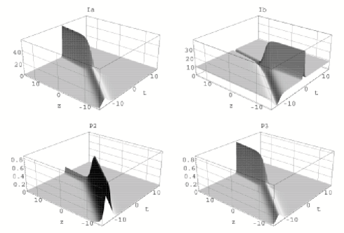
Figure 2: Knocking down the slow-light soliton. The two upper plots correspond to the dynamics of the intensities of the fields $\Omega_{a}$ and $\Omega_{b}$. The two lower plots show the populations of the levels $|2\rangle$ and $|3\rangle$. The parameters of plotted solutions are $c_{2}=c_{3}=1,\lambda_{0}=4.1i,\Delta=0$.

To this point we have described a mechanism of controlling the transparency of the medium for a particular type of slowly moving signals. We now discuss a possibility to read information stored in the atomic subsystem. Let us assume that the background field vanishes, i.e. $\Omega_{0}=0$. As was explained above, the speed of the slow-light soliton then vanishes as well. However, the information about polarization of the slow-light signal is stored in the atomic subsystem. This effect can be interpreted in terms of the concept of a polariton, which is a collective excitation of the overall atom-field system. The notion of a polariton for the $\Lambda$-system has been used before. In the linear case the dark-state polariton was discussed in Fleischhauer and Lukin (2000). In the strongly nonlinear regime, which is the case for the present work, a similar interpretation is possible. Indeed, the field component of a slow-light soliton solution can be interpreted as the light contribution into the slow-light polariton. When the controlling field $\Omega_{0}$ vanishes this contribution also vanishes, along with the speed of the polariton. The latter then contains only excitations in the atomic subsystem. The general solution Eqs.(30), (31) is then reduced to the form:

$$\tilde{\Omega}_{a}=\frac{2i\varepsilon_{0}\exp\left[{i\frac{\Delta\nu_{0}\zeta}{2(\varepsilon_{0}^{2}+\Delta^{2})}+i\log(\frac{c_{3}}{|c_{2}|})-i\varphi_{1}}\right]}{\cosh(\phi_{s0})+\frac{1}{2}\exp\left[{2\phi_{f0}-\phi_{s0}}\right]},$$

$$\tilde{\Omega}_{b}=e^{i\varphi_{1}+\log(c_{2})-\frac{i\nu_{0}\zeta}{2(\Delta+i\varepsilon_{0})}}\;\tilde{\Omega}_{a},$$ (50)

where $\phi_{s0}=\frac{\varepsilon_{0}\nu_{0}\zeta}{2(\Delta^{2}+\varepsilon_{0}^{2})}+\log(|c_{2}|)$ is the phase of the slow-light soliton, and $\phi_{f0}=\varepsilon_{0}\tau+\frac{\varepsilon_{0}\nu_{0}\zeta}{2(\varepsilon_{0}^{2}+\Delta^{2})}+\log(|c_{3}|)$ is the phase of the fast soliton for the vanishing background $\Omega_{0}$. The form of the fields resembles a superposition of fast and slow-light solitons in Eqs.(30), (31) with the vanishing velocity of the slow-light soliton. This last exponential term in the denominator represents the fast signal contribution. The component containing hyperbolic cosine describes the information about the slow-light soliton stored in the medium after the soliton was stopped. The overall picture of dynamics corresponds to the scattering of the fast soliton on this localized atomic polarization pattern. The atomic state describing this scattering reads

$$|\psi\rangle=-\left({\frac{i\varepsilon_{0}}{\sqrt{\Delta^{2}+\varepsilon_{0}^{2}}}\frac{e^{2\phi_{s0}}-1+e^{2\phi_{f0}}}{e^{2\phi_{s0}}+1+e^{2\phi_{f0}}}+\frac{\Delta}{\sqrt{\Delta^{2}+\varepsilon_{0}^{2}}}}\right)|1\rangle$$ (51)

$$+\frac{2i\,\varepsilon_{0}\exp\left[{i\left({\frac{\Delta\nu_{0}\zeta}{2(\varepsilon_{0}^{2}+\Delta^{2})}+\arg(c_{2})-\varphi_{1}}\right)+\phi_{s0}}\right]}{\sqrt{\Delta^{2}+\varepsilon_{0}^{2}}\;\left({e^{2\phi_{s0}}+1+e^{2\phi_{f0}}}\right)}\;|2\rangle-\frac{\tilde{\Omega}_{a}}{2\sqrt{\Delta^{2}+\varepsilon_{0}^{2}}}|3\rangle.$$

For $c_{3}=0$ the fields vanish, while the atomic state reduces to a form corresponding to a stopped polariton described by Eq.(47) with $\Omega_{0}=0$. In other words, when the slow-light soliton is completely stopped, the information borne by the soliton is stored in the spin polarization of the atoms. As long as the upper state $|3\rangle$ is not populated, the state of the atomic subsystem is not sensitive to the destructive influence of the optical relaxation processes.

The conventional way Liu et al. (2001) to read the information stored in the atoms is to increase the intensity of the background field. Our method of reading the information is different. We propose to send the fast soliton into the space domain in the active medium, where the information is stored. The polarization in the domain is then flipped by the fast signal. This is how the reading of information is realized. This way of reading optical information is advantageous because it involves fast easily detectable processes. Figure 3 illustrates the mechanism of the reading. Notice that the act of reading, based on the polarization flipping induced by the fast signal, can be realized on a very short time scale compared to typical relaxation times.

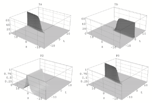
Figure 3: Reading the optical information by the fast soliton. The two upper plots illustrate the dynamics of the fields $\Omega_{a}$ and $\Omega_{b}$. The two lower plots show the populations of the levels $|2\rangle$ and $|3\rangle$. The standing peak on the plot for $P_{2}$ corresponds to the stored information in the form of the localized polarization. The rapidly moving localized excitation of the atoms given on the plot for $P_{3}$ represents the act of reading. The background field $\Omega_{0}=0$, and the coupling constant is the same as before, i.e. $\nu_{0}=4.5$.

IV Nonadiabatic manipulation of slow-light solitons

In this section we discuss an exactly solvable, though physical, case describing controlled preparation, manipulation and readout of slow-light solitons in atomic vapors and Bose-Einstein condensates. The group velocity of the slow-light soliton depends explicitly on the field $\Omega_{0}$, i.e. $v_{g}\approx c\frac{\Omega_{0}^{2}}{2\nu_{0}}$ (cf. Eq.(46)). This expression immediately suggests a plausible conjecture that when the controlling field is switched off the soliton stops propagating while the information borne by the soliton remains in the medium in the form of a spatially localized polarization pattern, i.e. optical memory, which can be recovered later. For brevity we refer to this pattern as to ”memory bit”.

Figure 4: The intensity of the field $\Omega_{b}$ as the function of time $t$. The thick solid curve shows the time-dependence of the controlling background field at entrance into the medium, i.e. at $z=0$. We also plot $|\tilde{\Omega}_{b}|^{2}$ at $z=6$ (dashed curve) and at $z=12$ (dotted curve). We choose $\alpha=4$, and the delay interval is $T-T_{1}=3$. The dimensionless units are defined in the text.

We consider the following scenario for the dynamics (see Fig.4). Before $\tau=0$ we create in the medium a slow-light soliton, and assume it is propagating on the constant background $\Omega_{0}$. We then slow-down the soliton by switching off the laser source of the background field. We assume an exponential decay of the background field with a decay constant $\alpha$, i.e. $\Omega_{0}e^{-\alpha\tau}$. At a certain moment of time, say, $T_{1}=4/\alpha$ the field becomes negligible. Therefore, we cut off the exponential tail and approximate it by zero. At this step the soliton is completely stopped. The position where the soliton stops, depends on the decay constant $\alpha$ and on the moment when we switch the laser off. The information borne by the soliton is stored in the form of spatially localized polarization. This formation can live a relatively long time in atomic vapors or BEC Dutton and Hau (2004). At the moment $T$ we restore the slow-light soliton by abruptly switching on the laser. The whole dynamics is divided into four time intervals $\bigcup_{i=0}^{3}{\cal D}_{i}=(-\infty,0]{\cup}[0,T_{1}]{\cup}(T_{1},T]{\cup}(T,\infty)$. The time-dependence of the intensity of the background field at entrance into the medium is given in Fig.4.

Before the soliton enters the medium, the physical system is assumed to be prepared in the state described by Eq.(9). The function $\Omega(\tau)$ now models switching the controlling field off and on again. This function reads (cf. Fig.4):

$$\Omega(\tau)=\Omega_{0}\left[\Theta(-\tau)+e^{-\alpha\tau}(\Theta(\tau)-\Theta(\tau-T_{1}))\right.$$ (52)

$$\left.+\Theta(\tau-T)\right].$$

Here $\Theta(\cdot)$ is the Heaviside step function with $\Theta(0)=\frac{1}{2}$. For the state Eq.(9) with Eq.(52) we exactly solve the nonlinear system Eqs.(5),(6) as well as the auxiliary scattering problem Eqs.(7), (8) underlying its complete integrability. The latter result is the cornerstone of analytical progress achieved in this section. This result allows to mounting a soliton on the background Eqs.(9),(52) using the Darboux-Bäcklund transformation described in section II (cf. Rybin and Vadeiko (2004)). According to the results of section II the one-soliton solution corresponding to the time dependent background Eq.(9) reads

$$\tilde{\Omega}_{a} = \frac{(\lambda^{*}-\lambda)w(\tau,\lambda)}{\sqrt{1+|w(\tau,\lambda)|^{2}}}\;e^{i\tilde{\theta}_{s}}\,\mathrm{sech}\tilde{\phi}_{s},$$ (53)

$$\tilde{\Omega}_{b} = \frac{(\lambda-\lambda^{*})w(\tau,\lambda)}{1+|w(\tau,\lambda)|^{2}}\,e^{\tilde{\phi}_{s}}\,\mathrm{sech}\tilde{\phi}_{s}-\Omega(\tau),$$

with the atomic state $\tilde{\rho}=|\tilde{\psi}_{at}\rangle\langle\tilde{\psi}_{at}|$, where

$$|\tilde{\psi}_{at}\rangle= \frac{\mathrm{Re}\lambda-\Delta-i\mathrm{Im}\lambda\tanh\tilde{\phi}_{s}}{|\lambda-\Delta|}|1\rangle$$ (54)

$$+\frac{\tilde{\Omega}_{a}}{2|\lambda-\Delta|w(\tau,\lambda)}|2\rangle-\frac{\tilde{\Omega}_{a}}{2|\lambda-\Delta|}|3\rangle.\quad$$

Here,

$$\tilde{\phi}_{s} = \tilde{\phi}_{0}+\frac{\nu_{0}\zeta}{2}\mathrm{Im}\frac{1}{\lambda-\Delta}+\mathrm{Re}(z(\tau,\lambda))$$

$$+ \ln\sqrt{1+|w(\tau,\lambda)|^{2}},$$

$$\tilde{\theta}_{s} = \tilde{\theta}_{0}-\frac{\nu_{0}\zeta}{2}\mathrm{Re}\frac{1}{\lambda-\Delta}+\mathrm{Im}(z(\tau,\lambda)),$$

where $\lambda$ is an arbitrary complex parameter. The functions $w(\tau,\lambda)$, $z(\tau,\lambda)$ are of piecewise form, specific to each time region ${\cal D}_{i}$.

Table 1: Exact analytical solution

${\cal D}$	$\Omega(\tau)$	$w(\tau,\lambda)$	$z(\tau,\lambda)$	${\cal C}$
${\cal D}_{0}$	$\Omega_{0}$	$w_{0}$	$\frac{i}{2}\Omega_{0}w_{0}\tau$	0
${\cal D}_{1}$	$\Omega_{0}e^{-\alpha\tau}$	$i\frac{{{\cal C}}J_{1-\gamma}\left(-\frac{\Omega(\tau)}{2\alpha}\right)-J_{\gamma-1}\left(-\frac{\Omega(\tau)}{2\alpha}\right)}{{\cal C}J_{-\gamma}\left(-\frac{\Omega(\tau)}{2\alpha}\right)+J_{\gamma}\left(-\frac{\Omega(\tau)}{2\alpha}\right)}$	$-\alpha\gamma\tau+\ln\frac{{{\cal C}}J_{-\gamma}\left(-\frac{\Omega(\tau)}{2\alpha}\right)+J_{\gamma}\left(-\frac{\Omega(\tau)}{2\alpha}\right)}{{\cal C}J_{-\gamma}(-\frac{\Omega_{0}}{2\alpha})+J_{\gamma}\left(-\frac{\Omega_{0}}{2\alpha}\right)}$	$\frac{-iw_{0}J_{\gamma}(-\frac{\Omega_{0}}{2\alpha})+J_{\gamma-1}(-\frac{\Omega_{0}}{2\alpha})}{J_{1-\gamma}(-\frac{\Omega_{0}}{2\alpha})+iw_{0}J_{-\gamma}(-\frac{\Omega_{0}}{2\alpha})}$
${\cal D}_{2}$	$0$	0	$\ln\frac{{\cal C}\left(-\frac{\Omega_{0}}{4\alpha}\right)^{-\gamma}/\mathrm{\Gamma}(1-\gamma)}{{\cal C}J_{-\gamma}(-\frac{\Omega_{0}}{2\alpha})+J_{\gamma}\left(-\frac{\Omega_{0}}{2\alpha}\right)}$	${\cal C}_{2}={\cal C}_{1}$
${\cal D}_{3}$	$\Omega_{0}$	$\frac{\Omega_{0}\tan\left({\frac{1}{2}\sqrt{\lambda^{2}+\Omega_{0}^{2}}(\tau-T)}\right)}{\lambda\tan\left({\frac{1}{2}\sqrt{\lambda^{2}+\Omega_{0}^{2}}(\tau-T)}\right)-i\sqrt{\lambda^{2}+\Omega_{0}^{2}}}$	$\begin{array}[]{c}\ln\frac{{\cal C}\,e^{\frac{-i\left({\lambda+\sqrt{\lambda^{2}+\Omega_{0}^{2}}}\right)(\tau-T)}{2}}+e^{\frac{-i\left({\lambda-\sqrt{\lambda^{2}+\Omega_{0}^{2}}}\right)(\tau-T)}{2}}}{{\cal C}+1}\\ +z_{2}\end{array}$	$\frac{\Omega_{0}^{2}+2\lambda\left({\lambda-\sqrt{\lambda^{2}+\Omega_{0}^{2}}}\right)}{\Omega_{0}^{2}}$

For clarity we organize elements of the solution corresponding to different time regions in Table 1. The function $w_{0}$ is defined as in Eq.(38) with $k=0$, the index of Bessel functions is defined as $\gamma=({\alpha+i\lambda})/({2\alpha})$. The values ${\cal C}_{i}$ of the constant ${\cal C}$ for each time region ${\cal D}_{i}$ are specified in the rightmost column of the table, the moment of time $T$ is chosen as in Fig.4, i.e. $T=4/\alpha+3$. Notice that in the table $w_{2}=w_{1}(\infty,\lambda)$ and $z_{2}=z_{1}(\infty,\lambda)$. Therefore the solution in the region ${\cal D}_{2}$ is parameterized by the asymptotic values of the data for the region ${\cal D}_{1}$ corresponding to the absence of cut-off of the exponentially vanishing tail. The region ${\cal D}_{2}$ describes the phase when the slow-light soliton is stopped: the fields vanish, while the information borne by the soliton is stored in the medium in the form of spatially localized polarization. At the time $T$ the laser is instantly turned on again. The stored localized polarization then generates a moving slow-light soliton. This process is described by the solution in the region ${\cal D}_{3}$. Except for the moment $T_{1}$, the functions $w,z$ are continuous in $\tau$. This ensures that the physical variables such as the wave-function and field amplitudes evolve continuously.

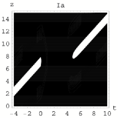
Figure 5: Contour plot of the intensity of $\tilde{\Omega}_{a}$. We choose $\lambda=-4.1i$ and zero detuning, $\Delta=0$. The break-up area in between the two solitonic trails manifests the creation of a standing memory bit in the medium.

We demonstrate typical dynamics of the intensity of the fields in Figs.4 and 5. In Fig.4 the decaying shock wave, whose front has an exponential profile, propagates with the speed of light, reaches the slow-light soliton and stops it. An intense and narrow peak is developing in the background field when the shock wave hits the soliton (dotted curve). This peak signifies a transfer of energy from the soliton to the background field. After the auxiliary laser has been switched on again, another step-like shock wave reaches the localized polarization formed in the medium by the incoming soliton, and retrieves stored information in the form of a new slow-light soliton. A narrow and deep depression in the intensity plot means now the energy transfers in the opposite direction, i.e. from the background field to the restored soliton. The dynamics of the field $\tilde{\Omega}_{a}$ is plotted in Fig.5. The contour plot shows that in the process of rapid deceleration the solitonic trail profiles end sharply. Notice that the characteristics of the restored pulse, i.e. the width and group velocity, are very close to those of the input signal existing in the medium before the stopping.

We now calculate the half-width of the polarization flip written into the medium after the soliton is completely stopped. It reads

$${\cal W}_{s}=4c\ln(2+\sqrt{3})\frac{|\Delta-\lambda|^{2}}{\nu_{0}\left|\mathrm{Im}(\lambda)\right|}.$$ (55)

It is important to notice that the width Eq.(55) of the optical memory formation does not depend on the rate $\alpha$. In other words, the width of the memory bit is not sensitive to how rapidly, i.e. nonadiabatically, the controlling field is switched off. This leads to an important conclusion. Indeed, through the variation of the experimentally adjustable parameter $\alpha$, it is possible to control the location of the memory bit, while its characteristic size remains intact. Dutton and Hau have already reported Dutton and Hau (2004) that when the switching is made quickly compared to the natural lifetime of the upper level, the adiabatic assumptions are no longer valid, but, remarkably, the quality of the storage is not reduced in the nonadiabatic regime. Our analytical result is in excellent agreement with this observation.

The group velocity of the slow-light soliton reads

$$\frac{v_{g}}{c}=\frac{|w(\tau,\lambda)|^{2}}{\frac{\nu_{0}(1+|w(\tau,\lambda)|^{2})}{2|\Delta-\lambda|^{2}}+|w(\tau,\lambda)|^{2}}.$$ (56)

Notice that in the case of the constant background field, i.e. in the case $\alpha=0$, the conventional expressions for the slow-light soliton Eqs.(43),(44) along with the expression for the group velocity Eq.(46) - the main motivational quantity for this report - can be readily recovered from Eqs.(53),(56).

The distance ${\cal L}_{s}(\alpha)$ that the slow-light soliton will propagate from the moment when the laser is switched off until the full stop, is

$${\cal L}_{s}(\alpha)=\frac{2c|\Delta-\lambda|^{2}}{\nu_{0}\mathrm{Im}(\lambda)}\,\tilde{\phi}_{s}|_{\tau=0}^{\tau=\infty}$$

$$= \frac{2c|\Delta-\lambda|^{2}}{\nu_{0}|\mathrm{Im}(\lambda)|}\left[\ln\sqrt{1+|w_{0}|^{2}}-\mathrm{Re}(z(\infty,\lambda))\right].\quad$$ (57)

It is evident from our solution Eq.(IV) that the soliton possesses some inertia or, in other words, a momentum of motion. Indeed, even if the controlling field is switched off instantly (notice that $\lim\limits_{\alpha\to\infty}\mathrm{Re}\,z(\infty,\lambda)=0$), the soliton will still propagate over some finite distance after the shock wave of the vanishing field, propagating with the speed of light, has reached the soliton.

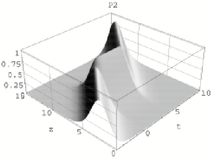
Figure 6: Population of level $|2\rangle$. Here, $\lambda=-4.1i$ and $\Delta=0$. The time interval $1\leq t\leq 4$ corresponds to a standing localized polarization flip. Compare with experimental results in Fig.1 of ref. Bajcsy et al. (2003).

In Fig.6 we show the dynamics of localized polarization corresponding to soliton dynamics shown in Fig.5. The plot is remarkably similar to the corresponding figure in reference  Bajcsy et al. (2003) describing recent experiments. The central part of the plot in Fig.6 shows the standing memory bit imprinted by the slow-light soliton. Notice that in the presence of the soliton the population flip from level $|1\rangle$ to $|2\rangle$ in the center of the peak is almost complete. This property of the solution manifests the major distinction between the strongly nonlinear regime considered in our paper and the linear EIT theory. As was already pointed out earlier Matsko et al. (2001); Dey and Agarwal (2003); Dutton and Hau (2004), the regime of two fields being comparable in magnitude opens up new avenues for an effective control over superposition of two lower states of the atoms. Changing the parameters of the slow-light soliton we can coherently drive the system to access any point on the Bloch sphere, which describes the lower levels. For zero detuning, the solution discussed here shows that when the field vanishes the maximum population of the second level reaches unity. Using Eq.(54) it is also not difficult to estimate the maximum population of the level $|2\rangle$ for finite detuning after the soliton was completely stopped: ${|\lambda|^{2}}/{|\Delta-\lambda|^{2}}$. Notice that only a small fraction of the total population is located in the upper level $|3\rangle$ and provides for some atom-field interaction. This population is proportional to $|\Omega_{0}|^{2}$. Numerical studies of the Maxwell-Bloch equations with relaxation terms included Dey and Agarwal (2003); Dutton and Hau (2004) show that for experimentally feasible group velocities of the slow-light pulses, i.e. when the maximum intensity of the controlling field is not very high, the pulses are stable against relaxation from level $|3\rangle$. Here we consider the same range of parameters. Therefore, the destructive influence of relaxation on our solution Eq.(53) is negligible.

V The case of arbitrary controlling field

In this section we build a single-soliton solution on the background of the state of the overall atom-field system described by Eq.(9) for a quit general (complex) controlling field $\Omega(\tau)$. The single-soliton solution corresponding to the background field $\Omega(\tau)$ is given by Eqs.(53),(54) with the functions $w(\tau,\lambda)$ and $z(\tau,\lambda)$ defined below.

We envisage the dynamics scenario similar to that of the previous section. We assume that the slow-light soliton is propagating in nonlinear superposition with the background field, which is constant at $\tau\to-\infty$ and vanishes at $\tau\to+\infty$. The speed of the slow-light soliton is controlled by the intensity of the background field. Therefore, when the background field decreases, the slow-light soliton slows down and stops, eventually disappearing and leaving behind a standing localized polarization flip, i.e. optical memory bit. Should the background field increase, the soliton will emerge again and accelerate accordingly.

To be specific, we define the asymptotic behavior for the field $\Omega(\tau)$ in the form

$$\Omega(\tau\rightarrow-\infty)=\Omega_{0},\;\Omega(\tau\rightarrow+\infty)=0.$$ (58)

The asymptotic boundary conditions Eq.(58) dictate the following asymptotic behavior for the functions $w(\tau,\lambda)$ and $z(\tau,\lambda)$ defined by Eqs. (27),(28):

$$w(-\infty,\lambda) = w_{0}=\frac{\Omega_{0}}{2k(\lambda)},\;w(+\infty,\lambda)=0,$$ (59)

$$z(-\infty,\lambda) = z_{0}\tau=i\frac{|\Omega_{0}|^{2}}{4k(\lambda)}\tau,$$ (60)

where $k(\lambda)=(\lambda+\sqrt{\lambda^{2}+|\Omega_{0}|^{2}})/2$. The function $z(\tau,\lambda)$ satisfying the asymptotical conditions Eq.(60) reads

$$z(\tau,\lambda)=z_{0}\tau+\int\limits_{-\infty}^{\infty}\left({\frac{i}{2}\Omega^{*}(\tau^{\prime})w(\tau^{\prime},\lambda)-z_{0}}\right)\Theta(\tau-\tau^{\prime})d\tau^{\prime}.$$ (61)

The function $w(\tau,\lambda)$ is defined by the relations

$$w(\tau,\lambda) = i\int\limits_{-\infty}^{\infty}e^{-i\,k(\tau-s)}\Theta(\tau-s)\tilde{w}(s,\lambda)\,ds,$$ (62)

$$\tilde{w}(\tau,\lambda) = \frac{\Omega(\tau)}{2}+\frac{1}{k^{2}}\left({\frac{|\Omega_{0}|^{2}}{4}k\,w-\frac{\Omega^{*}(\tau)}{2}(k\,w)^{2}}\right)\!.\quad$$ (63)

Here $\Theta(\tau)$ is the Heaviside step function. We rewrite the relations Eqs.(62),(63) in the form of nonlinear integral equation, viz.

$$\tilde{w}(\tau,\lambda)=\frac{\Omega(\tau)}{2}+\int\limits_{-\infty}^{\infty}e^{-i\,k(\tau-s)}\Theta(\tau-s)\tilde{w}(s,\lambda)\,ds$$

$$\cdot\int\limits_{-\infty}^{\infty}e^{-i\,k(\tau-s)}\Theta(\tau-s)\left({\frac{\Omega^{*}(\tau)}{2}\tilde{w}(s,\lambda)-\frac{|\Omega_{0}|^{2}}{4}}\right)\,ds.\quad$$ (64)

Hence, we can construct a solution $\tilde{w}(\tau,\lambda)$ iterating Eq.(V) and starting iterations from $\tilde{w}_{0}(\tau,\lambda)=\frac{1}{2}\Omega(\tau)$. Notice that the last term in Eq.(63) provides a correction of order $k^{-2}$, because the function $w(\tau,\lambda)$ asymptotically behaves as $1/k$. In the adiabatic regime when the background field varies slowly, i.e. all derivatives of $\Omega(\tau)$ are much smaller than $k$, we can integrate Eq.(62) by parts. Preserving only the lowest order term with respect to $k$ we obtain

$$w(\tau,\lambda)\approx\frac{\Omega(\tau)}{2k}.$$ (65)

Hence, at the lowest order in $k$ we find

$$z(\tau,\lambda)\approx z_{0}\tau+\int\limits_{-\infty}^{\infty}\left({\frac{i}{4k}|\Omega(\tau^{\prime})|^{2}-z_{0}}\right)\Theta(\tau-\tau^{\prime})d\tau^{\prime}.$$ (66)

As one can easily observe this expression is in agreement with the asymptotic condition Eq.(60).

For an arbitrary dependence of the background field on the retarded time $\tau$, the speed of the slow-light soliton can be represented in the following form:

$$\frac{v_{g}}{c}=\frac{\partial_{\tau}\,\phi_{s}}{\partial_{\tau}\,\phi_{s}-\partial_{\zeta}\,\phi_{s}}.$$ (67)

It can be readily seen that

$$\frac{\partial\phi_{s}}{\partial\tau}=\frac{\mathrm{Im}(\lambda)|w(\tau,\lambda)|^{2}}{1+|w^{(}\tau,\lambda)|^{2}},\;\frac{\partial\phi_{s}}{\partial\zeta}=\frac{\nu_{0}}{2}\mathrm{Im}\frac{1}{\lambda-\Delta}.$$ (68)

We have thus found a general solution for the velocity $v_{g}$ of the slow-light soliton propagating on an arbitrary time-dependent background field in terms of the function $\tilde{w}(\tau,\lambda)$ given by Eq.(V). This result provides a new way to study dynamics of localized optical signals in the nonlinear EIT systems. It allows us to easily suggest different schemes to slow-light down, stop, and reaccelerate slow-light solitonic contribution in the probing pulse. With such techniques one can introduce a concept of probing different regions of the media by changing the time that the soliton dwells at a particular location. This time is important in situations where the interaction between light and some impurities inside the EIT medium is weak and requires slowing the signal down in the vicinity of these impurities in order to gain more information about the structure of the medium.

We also introduce a notion of the distance ${\cal L}[\Omega]$ that the slow-light soliton will propagate until it fully stops. This quantity is important because it describes the location of an imprinted memory bit. The brackets $[\cdot]$ indicate a functional dependence of the distance on the controlling field $\Omega(\tau)$. To begin with we consider the case when the field is instantly switched off at the moment $\tau=0$, i.e. $\Omega(\tau)=\Omega_{0}\Theta(-\tau)$. Then we easily find the solution for $w$ and $z$:

$$w(\tau,\lambda)=w_{0}\left({\Theta(-\tau)+\Theta(\tau)\;e^{-i\lambda\tau}}\right),\;z(\tau,\lambda)=z_{0}\Theta(-\tau)\tau.$$

Hence, we can obtain the distance ${\cal L}_{0}$ that the soliton will propagate from the moment $\tau=0$ until its complete stop at $\tau\rightarrow\infty$:

$${\cal L}_{0}=\frac{c|\Delta-\lambda|^{2}}{\nu_{0}|\mathrm{Im}(\lambda)|}\ln\left(1+|w_{0}|^{2}\right).$$

Here we make use of the assumption that $\mathrm{Im}(\lambda)<0$.

Now, we can give the definition of the distance ${\cal L}[\Omega]$ for a generic field $\Omega(\tau)$ satisfying the conditions Eq.(58). It is convenient to define it as a relative distance, namely the difference between the absolute coordinate of the stopped signal at the maximum of the signal and the distance ${\cal L}_{0}$. The relative distance reads:

$${\cal L}[\Omega]=\frac{2c|\Delta-\lambda|^{2}}{\nu_{0}\mathrm{Im}(\lambda)}\!\!\int\limits_{-\infty}^{\infty}\mathrm{Re}\left({\frac{i}{2}\Omega^{*}(\tau)w(\tau,\lambda)-z_{0}\Theta(-\tau)}\right)d\tau.$$

Using the representation Eq.(63) we find

$${\cal L}[\Omega]=\frac{2c|\Delta-\lambda|^{2}}{\nu_{0}\mathrm{Im}(\lambda)}\mathrm{Re}\left({\int\limits_{-\infty}^{+\infty}\int\limits_{-\infty}^{+\infty}e^{-i\,k(\tau-s)}\Theta(\tau-s)\left({\frac{|\Omega_{0}|^{2}}{4}\Theta(-\tau)-\frac{\Omega^{*}(\tau)}{2}\tilde{w}(s,\lambda)}\right)ds\,d\tau}\right)_{.}$$ (69)

If we assume that $\Omega(\tau)$ is a smooth function and substitute the solution for $\tilde{w}(\tau,\lambda)$, we find the result in the form of a series

$${\cal L}[\Omega]=\frac{2c|\Delta-\lambda|^{2}}{2\nu_{0}\mathrm{Im}(\lambda)}\mathrm{Im}\left({\sum_{n=1}^{\infty}\frac{I_{n}}{k^{n}}}\right),$$

where $I_{n}[\Omega]$ are regularized Zakharov-Shabat functionals Faddeev and Takhtadjan (1987). The first two functionals read $I_{1}[\Omega]=-\int_{-\infty}^{\infty}\left({|\Omega(\tau)|^{2}-|\Omega_{0}|^{2}\Theta(-\tau)}\right)d\tau$, $I_{2}[\Omega]=\frac{1}{2i}\int_{-\infty}^{\infty}(\Omega^{*}(s)\partial_{s}\Omega(s)-\Omega(s)\partial_{s}\Omega^{*}(s))ds$. The other functionals can be obtained through the iteration procedure described above. As it is usual for the boundary conditions of finite density type, $I_{1}$ is not a proper functional on the complex manifold of physical observables, in the sense described in Faddeev and Takhtadjan (1987). In that sense all other functionals in the expansion with respect to $k$ are proper. It is a plausible conjecture that the minimum of the functional of length, Eq.(69), i.e. $\delta{\cal L}[\Omega]/\delta\Omega=0$ with $\delta^{2}{\cal L}[\Omega]/\delta\Omega^{2}>0$, is achieved when the controlling field is switched off instantly. Therefore it seems intuitively correct that the minimum is delivered by the the function $\Omega_{0}\Theta(-\tau)$ discussed above. This conjecture is also supported by the case discussed in section IV, when the controlling field vanishes exponentially, i.e. $\Omega(\tau)=\Omega_{0}(\Theta(-\tau)+\Theta(\tau)e^{-\alpha\tau})$. In this case the minimum of length is delivered by a singular limit $\alpha\to\infty$, i.e. in the regime of instant switching off of the controlling field.

Another important characteristics of the system is the shape of the imprinted signal. It is easy to show that the width ${\cal W}_{0}$ of the imprinted memory bit is not sensitive to the functional form of $\Omega(\tau)$ and is the same as given by Eq.(55). In other words, this exact result is valid regardless of how rapidly we switch the background field off. This means that specification of $\Omega(\tau)$ only influences the location of the stored signal and not its shape. This result is strongly supported by recent experiments Dutton and Hau (2004). This reference emphasizes the phenomenological fact that the quality of the storage is not sensitive to the regime of switching off of the control laser. Our exact result Eq.(55) provides a rigorous basis for this experimental observation.

To conclude this section we discuss the applicability of the concept of effective time to the regime of nonadiabatic variations of the controlling field. This concept was used before in Grobe et al. (1994); Bajcsy et al. (2003); Matsko et al. (2001) for approximative descriptions of pulse propagation on the background of a time-dependent controlling field. To account for this dependence, these references introduce an effective time variable (a ”scaled time” of ref.Bajcsy et al. (2003) and see the function $Z(\tau)$ of ref. Grobe et al. (1994) ). The reference Grobe et al. (1994)) shows the concept of effective (scaled) time to be very useful in the regime of linear EIT, while ref. Bajcsy et al. (2003) demonstrates applicability of this concept in the strongly nonlinear, though adiabatic, regime. The effective time approximation, in our formulation, is given by expressions Eqs.(65),(66) employed in the slow-light soliton solution Eqs.(53),(54). In Fig. 7 we compare the resulting approximate solution against an exactly solvable case discussed in section IV. We point out that the method of effective time has a rather limited applicability in the strongly nonlinear noadiabatic regime, which is most interesting for modern experiments Dutton and Hau (2004). Indeed, Fig. 7 demonstrates that this method as applied to the slow-light soliton gives rise to large errors in the regime of nonadiabatic dynamics. Therefore heuristic attempts Leonhardt (2004) to substitute an effective time into the slow-light soliton solution Eqs.(43),(44) is largely not accurate.

Figure 7: Here $\varepsilon_{0}=4.1$, $\Delta=0$, and $\Omega(\tau)=0.5e^{-4\tau}$. It is clear that when the background field changes relatively fast the exact solution given by solid and dotted lines are different from approximative one (dashed and dot-and-dash lines, correspondingly) by up to $40\%$.

VI Conclusions and discussion

In this paper we have discussed a physically realistic, exactly solvable model of manipulation, i.e. preparation, control and readout, of optical memory bits in the strongly nonlinear, and more importantly, nonadiabatic regime. We discussed a concept of the transparency gate for the slow-light solitons in a $\Lambda$-type medium. We explained how the fast soliton can destroy the slow-light soliton and close the gate for the latter. We also described the process of reading optical information, written into the active medium by the slow-light solitons. We have investigated a mechanism of dynamical control of the slow-light soliton whose group velocity explicitly depends on the background field. For a quite general background field, we found the location and shape of the memory bit written into the medium upon stopping the signal. Remarkably, the width of this spatially localized standing polarization flip is not sensitive at all to the functional form of the controlling field and is defined by the parameters of the slow-light soliton only.

It is worth discussing here a possibility to actually create in the $\Lambda$-type atomic medium the slow-light solitons. The general physical feature underlying the mathematical property of complete integrability is a delicate balance between the effects of dispersion and nonlinearity inherent in the medium. Provided that this balance is observed and the system is completely integrable, it is a general fact that virtually any sufficiently intensive localized initial condition creates solitons. The overall picture of nonlinear dynamics can be roughly described as follows. The evolving signal created by the incident pulse in the course of the dynamics separates into a number of solitons and a decaying tail. The latter vanishes in due course. The soliton-like signals survive (ideally, i.e. in the absence of dissipation) for infinitely long time. When the physical conditions underlying the complete integrability of the optical system are met, the general picture of the nonlinear dynamics is similar to that described above. Namely, a fairly arbitrary localized and intensive initial signal creates in the course of nonlinear dynamics a number of slow-light solitons. The number of slow-light solitons can be derived from the analysis of the corresponding zero-curvature representation. The signal Eqs.(43),(44) is a generic soliton-like solution of the nonlinear system Eqs.(5), (6) and therefore it is very plausible that such signal can be created. To conclude, we want to emphasize that in our considerations the distinguished role is assigned to the background field $\Omega(\tau)$ that turns out to be a nonlinear analog of the conventional controlling field appearing in the linear EIT formulation. The difference between the linear and nonlinear cases lies in the fact that in the nonlinear case the control field and the slow-light soliton solution are present in the same channel in an inseparable nonlinear superposition.

VII Acknowledgements

IV acknowledges the support of the Engineering and Physical Sciences Research Council, United Kingdom. Work at Los Alamos National Laboratory is supported by the USDoE.

References

- Hau et al. (1999) L. N. Hau, S. E. Harris, Z. Dutton, and C. H. Behroozi, Lett. to Nature 397, 594 (1999).
- Liu et al. (2001) C. Liu, Z. Dutton, C. H. Behroozi, and L. V. Hau, Lett. to Nature 409, 490 (2001).
- Phillips et al. (2001) D. F. Phillips, A. Fleischhauer, A. Mair, R. L. Walsworth, and M. D. Lukin, Phys. Rev. Lett. 86, 783 (2001).
- Bajcsy et al. (2003) M. Bajcsy, A. S. Zibrov, and M. D. Lukin, Lett. to Nature 426, 638 (2003).
- Braje et al. (2003) D. A. Braje, V. Balic, G. Y. Yin, and S. E. Harris, Phys. Rev. A 68, 041801(R) (2003).
- Mikhailov et al. (2004) E. E. Mikhailov, V. A. Sautenkov, Y. V. Rostovtsev, and G. R. Welch, J. Opt. Soc. Am. B 21, 425 (2004).
- Turukhin et al. (2002) A. V. Turukhin, V. S. Sudarshanam, M. S. Shahriar, and et al., Phys. Rev. Lett. 88, 023602 (2002).
- Bigelow et al. (2003) M. S. Bigelow, N. N. Lepeshkin, and R. W. Boyd, Science 301, 200 (2003).
- Soljacic and Joannopoulos (2004) M. Soljacic and J. D. Joannopoulos, Nature Materials 3, 213 (2004).
- Kocharovskaya et al. (2001) O. Kocharovskaya, Y. Rostovtsev, and M. O. Scully, Phys. Rev. Lett. 86, 628 (2001).
- Dutton and Hau (2004) Z. Dutton and L. V. Hau, Phys. Rev. A 70, 053831 (2004).
- Harris (1997) S. E. Harris, Phys. Today 50(7), 36 (1997).
- Lukin (2003) M. D. Lukin, Rev. Mod. Phys. 75, 457 (2003).
- Grobe et al. (1994) R. Grobe, F. T. Hioe, and J. H. Eberly, Phys. Rev. Lett. 73, 3183 (1994).
- Eberly (1995) J. H. Eberly, Quant. Semiclass. Opt. 7, 373 (1995).
- Andreev (1998) A. V. Andreev, JETP 86, 412 (1998).
- Dey and Agarwal (2003) T. N. Dey and G. S. Agarwal, Phys. Rev. A 67, 033813 (2003).
- Kozlov and Eberly (2000) V. V. Kozlov and J. H. Eberly, Opt. Commun. 179, 85 (2000).
- Dutton et al. (2001) Z. Dutton, M. Budde, C. Slowe, and L. V. Hau, Science 293, 663 (2001).
- Matsko et al. (2001) A. B. Matsko, Y. V. Rostovstsev, O. Kocharovskaya, A. S. Zibrov, and M. O. Scully, Phys. Rev. A 64, 043809 (2001).
- Faddeev and Takhtadjan (1987) L. D. Faddeev and L. A. Takhtadjan, Hamiltonian Methods in the Theory of Solitons (Springer, Berlin, 1987).
- Park and Shin (1998) Q.-H. Park and H. J. Shin, Phys. Rev. A 57, 4643 (1998).
- Byrne et al. (2003) J. A. Byrne, I. R. Gabitov, and G. Kovačič, Physica D 186, 69 (2003).
- Rybin and Vadeiko (2004) A. V. Rybin and I. P. Vadeiko, Journal of Optics B: Quantum and Semiclassical Optics 6, 416 (2004).
- Hioe and Grobe (1994) F. T. Hioe and R. Grobe, Phys. Rev. Lett. 73, 2559 (1994).
- Rybin et al. (1988) A. V. Rybin, V. B. Matveev, and M. A. Salle, Inverse Problems. 4, 173 (1988).
- Rybin (1991) A. V. Rybin, J. Phys. A: Math. and Gen. 24, 5235 (1991).
- Rybin and Timonen (1993) A. V. Rybin and J. Timonen, J. Phys. A: Math. And Gen. 26, 3869 (1993).
- Matveev and Salle (1991) V. B. Matveev and M. A. Salle, Darboux Transformations and Solitons in Springer Series in Nonlinear Dynamics (Springer Verlag, 1991).
- Fleischhauer and Lukin (2000) M. Fleischhauer and M. D. Lukin, Phys. Rev. Lett. 84, 5094 (2000).
- Leonhardt (2004) U. Leonhardt, Preprint ArXiv: quant-ph/0408046 (2004).