Preserving Quantum States Using Inverting Pulses : A Super-Zeno Effect

Abstract

We construct an algorithm for suppressing the transitions of a quantum mechanical system, initially prepared in a subspace ${\mathcal{P}}$ of the full Hilbert space of the system, to outside this subspace by subjecting it to a sequence of unequally spaced short-duration pulses. Each pulse multiplies the amplitude of the vectors in the subspace by $-1$. The number of pulses required by the algorithm to limit the leakage probability to $\epsilon$ in time $T$ increases as $T\exp[\sqrt{\log(T^{2}/\epsilon)}]$, compared to $T^{2}\epsilon^{-1}$ in the standard quantum Zeno effect.

Quantum computation is known to be more powerful than classical computation. Two well-known examples where quantum computation gives a clear advantage over the classical are searching and factorization. A key difference is that, only in the quantum case, one can use the possibility of destructive interference of quantum amplitudes to suitably design algorithms where one can cancel out the amplitudes of undesired states. We want to apply this general strategy to the problem of state preservation, i.e. how to limit the system’s evolution to a desired subspace ref1 .

Several different approaches to this question have been studied. Error-avoiding codes ref2 depend on existence of subspaces free of decoherence due to special symmetry properties, and error-correcting codes ref3 depend on monitoring the system and conditional feedback to achieve this. Another important strategy for state preservation is to use the well known quantum Zeno effect, studied by von Neumann, and others ref6 , viz. preserving a given quantum state by very frequent measurements. In fact, the reduction of wavefuction is not essential for the physics of the quantum Zeno effect, and one can achieve a similar suppression of transitions by suitably coupling the system strongly to an external system for short intervals in the bang-bang control ref4 and dynamical decoupling strategies ref5 , where the time evolution is always unitary, without any reduction of the wave-packet ref7 .

In this paper, we develop a bang-bang control type algorithm to preserve quantum states that involves unitary kicks interspersed with evolution according to the system-environment Hamiltonian for unequal time-intervals between between kicks. The unitary kicks we employ are inverting pulses similar to those used in Grover’s quantum search algorithm grover . The proposed algorithm does not require any symmetry properties and is much more efficient than the quantum Zeno effect. We will show that in our algorithm, the number of pulses required to keep the the quantum system in the same subspace up to time $T$ with probability greater than $1-\epsilon$ increases only as $T\exp[\sqrt{\log(T^{2}/\epsilon)}]$, for large $T$, and small $\epsilon$, whereas it varies as $T^{2}\epsilon^{-1}$ and $T^{2}\epsilon^{-1/2}$ for the quantum zeno effect with and without measurement. We shall call the preservation of state using such non-periodic pulse sequences the super-Zeno effect.

We consider a quantum mechanical system described by a finite dimensional Hilbert space ${\mathcal{H}}$, which is a direct sum of two orthogonal subspaces ${\mathcal{P}}$ and ${\mathcal{Q}}$. We assume that the system Hamiltonian $\mathbf{H}$ is bounded. The unitary operator corresponding to evolution for a time interval $t$ is given by $\mathbf{U}_{0}(t)=\exp[-i\mathbf{H}t]$. When the system is subjected to a very short duration external fields pulse, we assume that the effect of the pulse can be represented by a unitary operator ${\mathbf{J}}$. If the system is initially in the state $|\psi\rangle$, after being subjected to the pulse, its state is $\mathbf{J}|\psi\rangle$.

A sequence of $N$ pulses is specified by $(N+1)$ real numbers $\{x_{j}\},j=1{\rm~{}to~{}}N+1$, where $x_{j}t$ is the time-interval between the $j$th and $(j+1)$th pulse for $j=1$ to $N-1$, and $x_{N+1}t$ is the interval between the last pulse, and the measurement of the state of the system. Here $t$ is time interval between the initial preparation, and final measurement, and $\sum_{j=1}^{N+1}x_{j}=1$. In this case, the evolution operator is

$$\mathbf{W}_{N}(t)={\bf U}_{0}(x_{N+1}t){\mathbf{J}}\ldots{\mathbf{J}}{\bf U}_{0}(x_{2}t){\mathbf{J}}{\bf U}_{0}(x_{1}t).$$ (1)

Our aim is to choose a sequence of the time-intervals between pulses given by $\{x_{j}\}$, such that if the system is initially in a state $|\psi\rangle\in{\mathcal{P}}$, then the probability that the system is found in a state in ${\mathcal{Q}}$ after the pulse sequence is minimized.

In this paper, we shall discuss only the case where ${\mathbf{J}}$ is an inverting pulse: $\mathbf{J}=\mathbf{Q}-\mathbf{P}$, where $\mathbf{P}$ and $\mathbf{Q}$ are the projection operators for the subspaces ${\mathcal{P}}$ and ${\mathcal{Q}}$ respectively. Clearly, ${\mathbf{J}}|\psi\rangle=-|\psi\rangle$, if $|\psi\rangle\in{\mathcal{P}}$, and ${\mathbf{J}}|\psi\rangle=+|\psi\rangle$, if $|\psi\rangle\in{\mathcal{Q}}$. We first give an explicit construction of a recursively defined sequence ${\mathbf{U}}_{m}(t)$ (see Eq. (4) below), such that the transition amplitude $\langle q|{\mathbf{U}}_{m}(t)|p\rangle$ is ${\mathcal{O}}(t^{m+1})$. We then obtain quantitative bounds on the leakage probability, and compare the performance of our algorithm with the standard quantum Zeno effect.

The basic idea of using inverting pulses to produce destructive interference of quantum mechanical amplitudes and reduce the transition rate from a particular subspace to others is quite straight-forward. Let $|p\rangle$ be a general state in ${\mathcal{P}}$, and $|q\rangle$ a general state in ${\mathcal{Q}}$. Let ${\mathbf{U}}(t)$ be a unitary operator satisfying $\mathbf{U}(t)=\mathbf{I}+O(t)$ for $t\rightarrow 0$, where I is the identity operator and the matrix elements $U_{qp}$, and $U_{pq}$ are of $O(t^{r})$, with $r$ is a positive integer. Then in the transition amplitude $\langle q|\mathbf{U}(t)\mathbf{J}\mathbf{U}(t)|p\rangle$ a precise cancellation of the amplitude of ${\mathcal{O}}(t^{r})$ term occurs, and one gets

$$\langle q|\mathbf{U}(t)\mathbf{J}\mathbf{U}(t)|p\rangle=O(t^{r+1}).$$ (2)

Similarly, it is easy to see that if ${\mathbf{V}}(t)$ is an operator with $\mathbf{V}(t)=\mathbf{J}+O(t)$, then again a destructive interference of amplitudes to leading order occurs in $\langle q|\mathbf{V}(t)^{2}|p\rangle$, and if $V(t)_{qp}=O(t^{r})$, then,

$$\langle q|\mathbf{V}(t)^{2}|p\rangle=O(t^{r+1}).$$ (3)

Using this result, it is straight forward to construct a pulse sequence where the transition amplitude is ${\mathcal{O}}(t^{r})$ for any positive integer $r$ by recursion. We define operators $\mathbf{U}_{m}$ by the recursion relations

$${\bf U}_{m+1}(t) = {\bf U}_{m}(t/2)~{}{\mathbf{J}}~{}{\bf U}_{m}(t/2),{\rm~{}for~{}}m{\rm~{}even},$$ (4)

$$= {\bf U}_{m}(t/2)~{}{\bf U}_{m}(t/2),{\rm~{}for}~{}m{\rm~{}odd.}$$

with ${\bf U}_{0}={\bf U}_{0}(t)$. Then, by induction, it follows that the transition amplitude $\langle q|{\bf U}_{m}|p\rangle$ is of order ${\mathcal{O}}(t^{m+1})$.

We can write down $\mathbf{U}_{m}(t)$ explicitly as a product of $\mathbf{U}_{0}(t/2^{m})$’s and $\mathbf{J}$’s. For example

$$\mathbf{U}_{1}(t)=\mathbf{U}_{0}(t/2){\mathbf{J}}\mathbf{U}_{0}(t/2),$$

$$\mathbf{U}_{2}(t)=[\mathbf{U}_{0}(t/4){\mathbf{J}}\mathbf{U}_{0}(t/4)]^{2},$$

$$\mathbf{U}_{3}(t)=[\mathbf{U}_{0}(t/8){\mathbf{J}}\mathbf{U}_{0}(t/8)]^{2}{\mathbf{J}}[\mathbf{U}_{0}(t/8){\mathbf{J}}\mathbf{U}_{0}(t/8)]^{2}.$$ (5)

Let $N_{m}$ be the number of pulses used the sequence ${\mathbf{U}}_{m}$, then it is easily verified that

$$N_{m}=(2^{m+1}-2)/3,{\rm~{}for}~{}m{\rm~{}even},$$

$$=(2^{m+1}-1)/3,{\rm~{}for}~{}m{\rm~{}odd}.$$ (6)

We can derive quantitative bounds to estimate the probability of leakage out of the subspace ${\mathcal{P}}$ for this sequence $\mathbf{U}_{m}$. We will show that the leakage probability $L_{m}$ from subspace $\mathcal{P}$ to subspace $\mathcal{Q}$ for operator $\mathbf{U}_{m}$ applied for a total time $T$ is

$$L_{m}=\sum_{q\in Q}|\langle q|\mathbf{U}_{m}|p\rangle|^{2}\leq 2^{-m(m+1)}[ET]^{2m+2}.$$ (7)

Here $E=|\mathbf{H}|$, and we have used the definition of the norm of an operator $\mathbf{A}$, given by

$$|\mathbf{A}|={\genfrac{}{}{0.0pt}{}{\mathrm{Sup}}{\psi}}\ ||\mathbf{A}|\psi\rangle||~{}/~{}||~{}|\psi\rangle||$$ (8)

By making $m$ large, $L_{m}$ can be made as small as we please. This becomes a state preservation algorithm when the subspace ${\mathcal{P}}$ consists of just the initial state. Note that the minimum time interval between pulses decreases as $2^{-m}T$, and this may limit the maximum value of $m$ that can be realized in an experimental setup.

For the $m$-th sequence, , the leakage probability varies as $2^{-m^{2}}$, while the number of pulses increases as $2^{m}$. Thus, the leakage probability varies as $\exp[-(\log N)^{2}]$. In Fig. 1, we have plotted the upper bound on leakage probability $L_{m}$ as a function of the number of pulses $N_{m}$. For comparison, we have also shown the corresponding bound on the leakage probability for same number of pulses for the quantum Zeno effect, both with repeated measurements, and with unitary evolution with periodic inversion pulses. For the last two, these bounds are $(ET)^{2}/N$ and $(ET)^{4}/N^{2}$ rspectively ( see discussion below). The improvement in the super-Zeno over the others is quite large, even for fairly small values of $m$; e.g. for $ET=1$ and $m=4$, which corresponds to only $10$ pulses, the leakage probability is already of order $10^{-4}$.

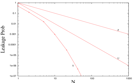
Figure 1: The plot of the upper bounds to the leakage probability versus the number of pulses. The curves are marked Z for the Zeno with periodic measurement, U for unitary evolution with periodic pulses, and S for the Super-Zeno cases, for $ET=1$. Here $T$ is the total time for evolution, and $E$ is the norm of the hamiltonian.

To prove the inequality (7), define

$$B_{m}(t)=\genfrac{}{}{0.0pt}{}{{Max}}{|p\rangle|q\rangle}~{}~{}|\langle q|\mathbf{U}_{m}(t)|p\rangle|=|\mathbf{Q}\mathbf{U}_{m}\mathbf{P}|$$ (9)

We have already seen that $B_{m}$ is ${\mathcal{O}}(t^{m+1})$. Since the only available timescale is $1/|{\mathbf{H}}|$, and $B_{m}$ is bounded by $1$ for large $t$, we can choose constant $K_{m}$ such that

$$B_{m}(t)\leq K_{m}(Et)^{m+1},{\rm~{}for~{}~{}all}~{}t.$$ (10)

The proof of Eq.(7) is complete if we can show that

$$K_{m}\leq 2^{-m(m+1)/2}.$$ (11)

This can be proved using the following simple mathematical inequalities valid for all mutually orthogonal projection operators $\mathbf{P}$ and $\mathbf{Q}$, and all unitary operators $\mathbf{U}$ and $\mathbf{V}$, with ${\mathbf{J}}={\bf Q}-{\bf P}$ (proof omitted):

$$|\mathbf{Q}\mathbf{U}\mathbf{J}\mathbf{U}\mathbf{P}|\leq~{}2~{}|\mathbf{Q}\mathbf{U}\mathbf{P}|~{}\mathrm{Min}[1,~{}|\mathbf{U-I}|~{}],$$ (12)

and

$$|\mathbf{Q}\mathbf{VV}\mathbf{P}|\leq~{}2~{}|\mathbf{Q}\mathbf{V}\mathbf{P}|~{}\mathrm{Min}[1,~{}|\mathbf{V}-\mathbf{J}|~{}].$$ (13)

Putting $\mathbf{U=U}_{r-1}$, with $r$ odd, and ${\mathbf{V}}={\mathbf{U}}_{r-1}$ with $r$ even, then using $|{\mathbf{U}}-{\mathbf{I}}|\leq Et$ and $|{\mathbf{V}}-{\mathbf{J}}|\leq Et$ in the inequalities above, we get

$$K_{r}\leq 2^{-r}K_{r-1}.$$ (14)

This, together with $K_{0}=1$, implies Eq.(11), and completes the proof of Eq.(7).

We now compare the performance of our algorithm with that of state preservation using the standard Zeno effect. Let $C(T,\epsilon)$ be the minimum number of pulses required to keep a quatum system in a precribed state for time $T$, with the leakage probability less than $\epsilon$. It seems reasonable to take this as the measure of the cost of algorithm.

Recall that in the standard quantum Zeno effect, starting with an initial state $|p\rangle$, and measuring the projector $|p\rangle\langle p|$ repeatedly, at times $T/N$, $2T/N$, $\cdots$, $T$, the probability of finding the system in the state $|p\rangle$ in each of these measurements is $S(T)=|\langle p|e^{-i\mathbf{H}T/N}|p\rangle|^{2N}$. For small $T/N$, we can approximate this as $[1-A(T/N)^{2}]^{N}\leq(1-AT^{2}/N)$, where $A=\langle p|{\bf H}^{2}|p\rangle-\langle p|{\bf H}|p\rangle^{2}\leq E^{2}$. Thus the leakage probability is has an upper bound $(ET)^{2}/N$, and $C(T,\epsilon)$ varies as $T^{2}/\epsilon$.

If we use $N$ equispaced unitary kicks ${\mathbf{J}}$ in time $T$, the cost $C(T,\epsilon)$ varies as $T^{2}/\sqrt{\epsilon}$. This follows from the fact that the magnitude of the transition amplitude from subspace ${\mathcal{P}}$ to ${\mathcal{Q}}$ after two pulses is $\leq(ET)^{2}/N^{2})$, and , the magnitude of the transition amplitude after $N$ pulses, and not the transition probability, has an upper bound $(ET)^{2}/N$.

In our case, the number of pulses $N_{m}$ varies as $2^{m}$, and the leakage probability varies as $\exp(-m^{2})$, for large $m$. Hence, for fixed $T$ and large $m$, the leakage probability $L_{m}$ decreases as $2^{-(\log_{2}N)^{2}}$. Equivalently, for fixed $T$,as $\epsilon$ is decreased, $C(T,\epsilon)$ increases as $\exp(K\sqrt{\log(1/{\epsilon})})$, where $K$ is a constant. This is slower than any power law in $\epsilon$.

Now we discuss the behavior of $C(T,\epsilon)$ for large $T$. In this case, Eq.(7) implies that $C(T,\epsilon)$ increases at most as $T^{2}$ for large $T$. However, for large $T$, the bound Eq.(7) is too weak, and we can prove the stronger result

$$C(T,\epsilon)\leq KET~{}2^{\sqrt{\log_{2}(E^{2}T^{2}/\epsilon)}},$$ (15)

where $K$ is some constant.

We indicate the proof here. Consider $2^{r+1}>ET>2^{r}$, where $r$ is a non-negative integer. Assume $m\geq r$. From the first halves of inequalities (12) and (13), $B_{m}(T)\leq 2^{r}B_{m-r}(T/2^{r})$. Then using the bound (7) for $B_{m-r}$, we get

$$B_{m}(T)\leq 2^{r}(ET2^{-m})^{m-r+1}2^{\frac{(m-r)(m-r+1)}{2}}.$$ (16)

On taking logs, the inequality $B_{m}\leq\sqrt{\epsilon}$, becomes a quadratic inequality for $m$, which is easily solved to give

$$m\geq\log_{2}(ET)+\sqrt{\log_{2}(E^{2}T^{2}/\epsilon)}+{\mathcal{O}}(1),$$ (17)

for $ET\gg 1$. Since the number of pulses increases as $2^{m}$, we get Eq.(15).

Our result is similar to that found by Khodjasteh and Lidar khodjasteh , who also used a recursive construction of pulse sequences, and found it to be better than the periodic pulse sequence. They considered pulse sequences for preservation of quantum states which work for all initial states, and the pulse sequence is independent of the state to be preserved. However, they require more than one type of pulses to achieve this. In contrast, we allow only one type of pulses, and can only minimize the leakage probability out of a subspace, and the pulse depends on the subspace to be preserved.

We note that in our construction, the intervals between pulses take only two values, one of which is twice the other. This may be convenient in actual implementation, as one can start with a source that generates periodic field pulses of the desired type, and then selectively block some of the pulses. There is no problem in relaxing the assumption about pulse-width being infinitesimal. In fact, if the inverting pulse is error-free, then one can just use a periodic repetition of inverting pulses to get a perfect preservation of the state. Effect of noise in the inverting pulse would strongly affect the performance of the algorithm, and remains to be studied.

It is possible to decrease the required number of pulses significantly if we allow the intervals between pulses to be varied continuously independent of each other. In general, one can try to find non-negative $(N+1)$ real numbers $\{x_{j}\}$, such that for the matrix ${\mathbf{W}}_{N}(t)$ defined in Eq.(1), the transition amplitude $\langle q|\mathbf{W}_{N}(t)|p\rangle$ is of a specified order $\mathcal{O}(t^{m+1})$, as $t\rightarrow 0$. This is certainly possible, by our explicit construction, for $N=N_{m}$. Also, if this is possible to do for one value of $N=r$, it is also possible for $N=r+1$, as one can always add the $(r+1)$-th pulse at the end of time $T$, with $x_{r+2}=0$. Hence we have proved that for any $m\geq 0$, there is an integer $N_{min}(m)$, such that for all $N\geq N_{min}(m)$, one can find an $N$- pulse sequence $\mathbf{W}_{N}(t)$ such that the transition amplitude $\langle q|\mathbf{W}_{N}(t)|p\rangle$ is $\mathcal{O}(t^{m+1})$, for small $t$.

Clearly, $N_{min}(m)\leq N_{m}$. We can improve this bound using a variation of the recursive construction of reflection-symmetric sequences ( i.e. those for which $x_{j}=x_{N+2-j}$, for all $j$) due to Yoshidayoshida . For such sequences, we have $\mathbf{W}_{N}(t)\mathbf{W}_{N}(-t)={\mathbf{I}}$ for all $t$. This implies that if $\langle q|\mathbf{W}_{N}(t)|p\rangle={\mathcal{O}}(t^{r})$, then $r$ must be odd. Then construct

$$\mathbf{W}^{\prime}(t)=\mathbf{W}_{N}(\alpha t){\mathbf{J}}\mathbf{W}_{N}(\beta t){\mathbf{J}}\mathbf{W}_{N}(\alpha t),$$ (18)

with $\alpha=1/(2+2^{\frac{1}{r}}),\beta=1-2\alpha$. Then it is easily checked that the ${\mathcal{O}}(t^{r})$ term in $\langle q|\mathbf{W}^{\prime}|p\rangle$ vanishes by construction. Hence the leading term in $\langle q|\mathbf{W}^{\prime}|p\rangle$ must be the next odd term, i.e. ${\mathcal{O}}(t^{r+2})$. Starting with number of pulses $N_{r}=0$ for $r=1$, we can recursively construct a sequence where the transition amplitude is ${\mathcal{O}}(t^{2m+1})$ uses only $3^{m}-1$ pulses. Thus, we get $N_{min}(2m)\leq 3^{m}-1$, which is a significant improvement over $N_{min}(m)\leq N_{m}$.

Further improvements are posible. For a given $N$, one can express $\langle q|{\bf W}_{N}(t)|p\rangle$ as Taylor series in powers of $t$. The coefficients of different powers of $t$ are sums of matrix-elements of the type $\langle q|{\bf H}^{n_{1}}{\mathbf{J}}{\bf H}^{n_{2}}{\mathbf{J}}..|p\rangle$, with coefficients that are polynomials of $\{x_{j}\}$. We try to set all such coefficients for powers of $t$ up to $m$ equal to zero, and solve the resulting polynomial equations for $\{x_{j}\}$. This calculation is straight forward for small $m$. For $m=0,1$ and $2$, the sequences we get are $\bf U_{0},\bf U_{1}$ and $\bf U_{2}$. For larger $m$, $\bf U_{m}$ or the ${\bf W}^{\prime}$ are not optimal.

The number of polynomial equation for equating to zero all terms up to order $m$ are $(2^{m}-1)$. Interestingly, one can find a much small number of variables $\{x_{j}\}$ that do satisfy all of these. In particular, for $m=5$, we can find six positive real numbers $x_{1},\ldots x_{6}$ that satisfy all the $31$ equations generated. For still higher $m$, the equations become rather messy to analyse, even with Mathematica. However, in the cases that we could solve, the final solution is surprizing simple. We omit the details, only mention here that for $m=4$, the optimizing pulse sequence is $\{x_{j}\}=\{\beta,1/4,1/2-2\beta,1/4,\beta\}$ with $\beta=(3-\sqrt{5})/8$. For $m=5$, it is $\{\gamma,1/4-\gamma,1/4,1/4,1/4-\gamma,\gamma\}$, with $\gamma=(\sqrt{3}-1)/4$. We find that while $N_{min}(m)=m$ for $0\leq m\leq 5$, but $N_{min}(6)>6$.

We note that the optimal sequences $\{x_{j}\}$ have been defined in terms of ${\bf H}$ and ${\mathbf{J}}$, but the polynomial equations, and therefore the roots, actually do not depend on them at all! A more direct characterization of these has not been possible so far. Similar sequences have been studied earlier in the context of finding efficient numerical integration techniques in classical mechanics using symplectic integration donnelly . In quantum Monte Carlo studies, the hamiltonian $\mathbf{H}$ of the system can often be expressed as a sum of two mutually non-commuting terms : $\mathbf{H}=\mathbf{A+B}$, such that there are efficient procedures to apply the operators $e^{t{\bf A}}$ and $e^{t{\bf B}}$ to a given state. Then using a generalization of the well-known Trotter formula, the propagator of the full hamiltonian is approximated as

$$e^{t\mathbf{A}+t{\mathbf{B}}}=e^{x_{1}tA}e^{x_{2}tB}e^{x_{3}tA}\ldots e^{x_{N}tB}+\mathcal{O}(t^{m}).$$ (19)

To make the discretization error small, one wants to choose the parameters $x_{1},x_{2}\ldots$ to maximize $m$ suzuki . If we write $-i\mathbf{H=A}$ and $-i\mathbf{JHJ=B}$, then ${\mathbf{J}}e^{-itx_{j}{\mathbf{H}}}{\mathbf{J}}=e^{tx_{j}{\mathbf{B}}}$, and ${\mathbf{W}}_{N}(t)$ is of the form Eq(19). In the quantum Monte Carlo case, it has been proved that for $m\geq 4$, one cannot find a solution with all $\{x_{j}\}$ non-negative suzuki2 . In our problem, the inversion pulse provides some crucial changes of sign in the algebraic equations, making the construction of pulse sequences using non-negative $\{x_{j}\}$’s possible for arbitrary $m$.

To summarize, in this paper, we have presented an algorithm for preserving quantum states using inverting pulses, with unequal time interval betwen pulses, which does not assume any symmetry properties of the Hamiltonian. The significant improvement over the quantum Zeno effect leakage probability seems promising for applications to efficient preservation of quantum states against decoherence, in quantum computations and communications. On the theoretical side, the asymptotic behavior of $N_{min}(m)$ for large $m$ is an interesting problem for further study.

DD would like to thank Prof. V. Singh and Prof. D.-N. Verma for very enlightening discussions, and Sumedha for help with Mathematica. We thank the referees, and K. Damle, R. Godbole, T.R. Ramadas and M. Randeria for their suggestions for improvement of the presentation of the paper.

References

- (1) See e.g., D. P. DiVincenzo, Science 270 225 (1995); P. W. Shor et al; ibid, 270 1633 (1995); A. Ekert, and R. Josza, Rev. Mod. Phys. 68 733 (1996).
- (2) P. Zanardi and M. Rasetti, Phys. Rev. Lett. 79 3306 (1997).
- (3) P. W. Shor, Phys. Rev. A 52, R 2493 (1995); J. I. Cirac, A. K. Ekert and C. Macchiavello, Phys. Rev. Lett.,82 4344 (1999); A. R. Calderbank, E. M. Rains, P. W. Shor, and N. J. A. Sloane, Phys. Rev. Lett. 78, 405 (1997); C. H. Bennett, D. P. DiVincenzo, and J. A. Smolin, ibid., 78, 3217 (1997).
- (4) J. von Neumann, Mathematical Foundations of Quantum Mechanics, Princeton Univ. Press (1955), p. 364; L. Fonda, G. C. Ghirardi and A. Rimini, Rep. Progr. Phys. 41, 587 (1978); B. Misra and E.C.G. Sudarshan, J. Math. Phys. 18, 756 (1977); A. P. Balachandran and S.M. Roy, Phys. Rev. Lett. 84, 4019 (2000); A.G. Kofman and G. Kurizki, Nature 405, 546 (2000).
- (5) L. Viola and S. Lloyd, Phys. Rev A 58, 2733(1998).
- (6) L. Viola, E. Knill and S. Lloyd, Phys. Rev. Lett. 82, 2417 (1999); ibid 85, 3520 (2000); L. Viola, S. Lloyd and E. Knill, Phys. Rev. Lett., 83 4888 (1999).
- (7) P. Facchi, D. A. Lidar and S. Pascazio, Phys. Rev., A69,032314 (2004).
- (8) L. K. Grover, Phys. Rev. Lett. 79, 325 (1997).
- (9) K. Khodjasteh and D. A. Lidar, Phys. Rev. Lett. 95, 180501 (2005).
- (10) H. Yoshida, Phys. Lett. A 150, 262 (1990).
- (11) D. Donnelly, E. Rodgers, Amer. J. Phys., 73 938(2005).
- (12) M. Suzuki, Phys. Lett. A 165 (1972) 1183; N. Hatano and M. Suzuki, in Quantum Annealing and related Optimization Methods, Lecture Notes Phys. vol. 679, A. Das and B. K. Chakrabarti (Eds.)[Springer, Heidelberg, 2005][arXiv:math-ph/0506007]
- (13) M. Suzuki, Phys. Lett. A 201,400 (1991).