Quantum transducers: Integrating Transmission Lines and Nanomechanical Resonators via Charge Qubits

Abstract

We propose a mechanism to interface a transmission line resonator (TLR) with a nano-mechanical resonator (NAMR) by commonly coupling them to a charge qubit, a Cooper pair box with a controllable gate voltage. Integrated in this quantum transducer or simple quantum network, the charge qubit plays the role of a controllable quantum node coherently exchanging quantum information between the TLR and NAMR. With such an interface, a quasi-classical state of the NAMR can be created by controlling a single-mode classical current in the TLR. Alternatively, a “Cooper pair” coherent output through the transmission line can be driven by a single-mode classical oscillation of the NAMR.

I Introduction

Solid state systems are promising candidates for novel scalable quantum networks Div . However, intrinsic features of solid-state-based channels, such as finite correlation length and environment-induced decoherence, may limit this scalability. Thus, it is crucial to coherently connect two or more quantum channels by using suitable quantum nodes. Coherently interfacing two quantum systems requires a high fidelity transfer of quantum states between them.

Here we describe a physical mechanism for interfacing a nanomechanical resonator (NAMR) (see, e.g.,  nature1 ; nature2 ; sq ; schwab ; zoller ; pra1 ) and a superconducting transmission line resonator (TLR) pra1 , i.e., a quantum transducer between mechanical and electrical signals. With increasing quality factors (e.g., $Q\approx 10^{3}-10^{5}$) and large eigenfrequencies (e.g., $\omega_{b}\approx$ MHz - GHz), NAMRs have been fabricated in the nearly quantum regime and proposed as candidates for either entangling two JJ qubits  armour_PRL_2002 ; cleland , or demonstrating progressive quantum decoherence wang . A superconducting TLR has recently been demonstrated yale_nature_2004 as a quantized boson mode strongly coupled to a Josephson junction (JJ) charge qubit DML . Many new possibilities can be explored for studying the strong interaction between light and macroscopic quantum systems (see, e.g., you01 ). In principle, the quantized boson modes of NAMRs and TLRs can be regarded as quantum data buses (see, e.g., wei_EPL_2004 ). Also, theoretical proposals have been made for interfacing these with optical qubits tian1 ; tian2 ; lukin1 .

Here we investigate the quantum integration of solid-state qubits and their data buses. In particular, we study how to connect two very different quantum channels, a mechanical and an electrical, provided by the NAMR and TLR, through a quantum node implemented by a Cooper pair box (CPB) or charge qubit. Our system can be considered the quantum analog of the transducer found in classical telephones (mechanical vibrations converted into electrical signals and vice versa). Because these three quantum objects (NAMR, TLR, and CPB) have been respectively realized experimentally with fundamental frequencies of the same order, it is quite natural to expect that they can be effectively coupled with each other. The physical principle behind our approach is similar to a theoretical prediction from cavity QED Slesh : Interacting with a common two-level atom, two off-resonant boson fields can be effectively entangled and then the quantum state tomography of a mode can be done with a high fidelity from the output of another. We similarly use the charge qubit as an artificial atom to coherently link two kinds of boson modes, the TLR and the NAMR ones. This quantum-node-induced interaction is controllable and can be freely switched-on and -off. A direct TLR and NAMR coupling through the gate voltage is problematic because the on-chip coupling cannot be easily controlled.

The physical mechanism, describe below, to prepare the quasi-classical state of the NAMR has an atomic cavity QED analogue. Consider an atom located in an optical resonator, and a classical pump laser also going through the cavity Slesh . The atom interacts with the cavity field and the laser, and therefore couples the classical laser to the quantized cavity field. When the atom is off-resonance with respect to the cavity, the cavity mode can behave as a forced harmonic oscillator, where the external force is effectively supplied by the classical laser. Thus, the coherent state of the cavity mode can be generated and controlled by the driving laser. This analogy motivates us to consider an inverse of the above scheme generating the NAMR coherent state. We set the TLR in a classical oscillation with a single frequency. This oscillation plays the role of the classical pump laser in the case of cavity QED. The off-resonant charge qubit interacts with both the NAMR and TRL, and thus induces an external force on the NAMR. This force will drive the boson mode of the NAMR into a coherent state.

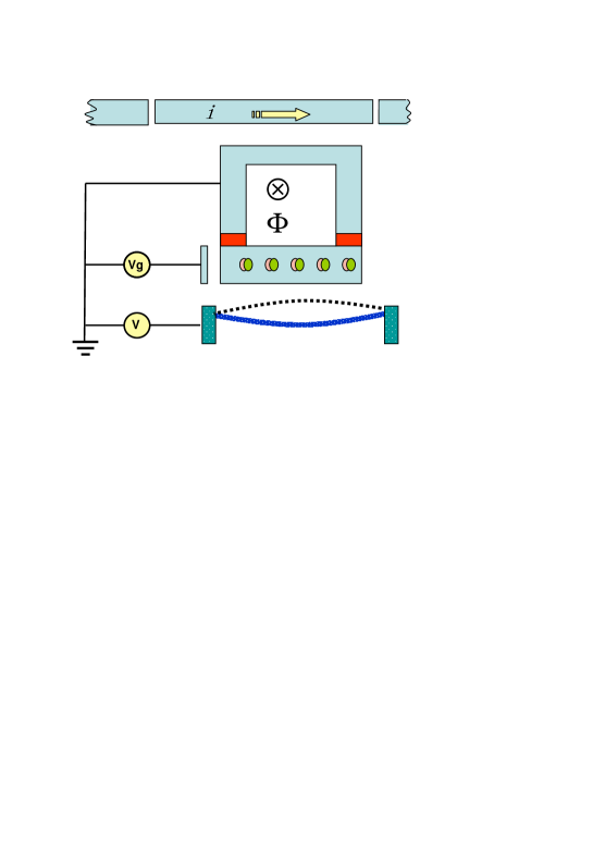
Figure 1: Schematic diagram of the coupled system of a Nanomechanical resonator (NAMR) and Transmission line resonator (TLR). The TLR is located right above the SQUID connected to the Cooper-pair box (CPB), so the TLR can produce a flux threading the loop in the SQUID. The Cooper-pairs are schematically represented by two small overlapping circles inside the Cooper-pair box. The NAMR is shown right below the CPB. The CPB acts as a transducer mediating the interaction between the NAMR and the TLR.

II Model

The proposed transducer is illustrated in Fig. 1. A horizontal TLR is fabricated coplanar with a CPB. The charge state of the CPB can be controlled by the gate voltage $V_{g}$ applied to the gate capacitor $C_{g}$. The CPB is also coupled to a large superconductor, the thermal bath, through two JJs with tunnelling energy $E_{J}$. The SQUID geometry also allows to apply external magnetic fluxes to control the charge state of the CPB. A NAMR (at the bottom of Fig. 1) with fundamental frequency $\omega_{b}$ and mass density $m$ is coupled to the CPB through the distributed capacitance $C(x)$, which depends on the displacement

$$x=\sqrt{\frac{1}{2m\omega_{b}}}(b^{{\dagger}}+b)$$

quantized by $[b,b^{{\dagger}}]=1$.

Let us assume that the distance fluctuations of the NAMR are much smaller than the distance $d$ between the NAMR and the CPB. Thus, the generic formula $C_{d}=\varepsilon A/d$ of the parallel plate capacitance, with effective area $A$, becomes $C\left(x\right)\simeq C_{0}(1-x/d)$, where $C_{0}$ is the distributed capacitance of the NAMR in equilibrium. It is the $x$-dependence of $C\left(x\right)$ that couples the CPB to the  NAMR, with free Hamiltonian $H_{n}=\omega_{b}\,b^{{\dagger}}b$. For small Josephson junctions, we assume that the equilibrium capacitance $C_{0}$ and the gate one $C_{g}$ are much less than $C_{J}$. In the neighborhood of $n_{g}=(C_{g}V_{g}+C_{0}V)/(2e)=1/2,$ the joint system (CPB and NAMR) can be approximately described by an effective spin-boson Hamiltonian

$$H_{1}=\frac{\omega}{2}\sigma_{z}^{\prime}+\omega_{b}\,b^{{\dagger}}b+\lambda(b^{{\dagger}}+b)\sigma_{z}^{\prime}-\frac{E_{J}}{2}\cos\left(\frac{\pi\Phi_{x}}{\Phi_{0}}\right)\,\sigma_{x}^{\prime}$$ (1)

where $\omega=4E_{C}(2n_{g}-1)$, $E_{C}=e^{2}/(2C_{T})$, and

$$\lambda=\frac{e\,C_{0}\,V}{C_{T}\,d\,\sqrt{2\,m\,\omega_{b}}}.$$

Above, we have neglected the high frequency term proportional to $x.$ $C_{T}=C_{J}+C_{g}+C_{0}$ is the total effective capacitance. The Pauli matrices ($\sigma_{x}^{\prime},\sigma_{y}^{\prime},\sigma_{z}^{\prime})$ of the quasi-spin are defined with respect to two isolated charge states, $\left|1\right\rangle$ and $\left|0\right\rangle$, of the CPB.

The coupling between the CPB and the TLR results from the total external magnetic flux $\Phi_{x}=\Phi_{C}+\Phi_{q}$ through the SQUID loop of effective area $S$ $(\approx 1\mu m^{2})$. Here, $\Phi_{c}$ is a classical flux used to control the Josephson energy and $\Phi_{q}=S\mu_{0}I_{\max}/(2\pi r)$ is the quantized flux arising from the quantization of the current $I$ in the TRL. We assume that the SQUID is placed near the point where the amplitude of the magnetic field is largest; $r$ $(\approx 10\,\mu m)$ is the distance between the line and the SQUID, and $\mu_{0}\,(=4\pi\times 10^{-7}{\rm H\,m}^{-1})$ is the vacuum permeability. The quantized current in the TLR can be directly obtained from the quantization of the voltage (see, e.g., Ref. pra1 ) through the continuous Kirchhoff’s equation $\partial_{z}I(z,t)=-c\,\partial_{t}V(z,t).$ At the anti-node $z=L/(2k)$, the quantized current $I(z,t)$ takes its maximum amplitude $I_{\max}$ to create a quantized flux

$$\Phi_{q}=i\sum_{k}\phi_{k}(a_{k}-a_{k}^{{\dagger}}),\,\,\phi_{k}=\sqrt{\frac{2c}{(k\pi)^{3}\,\nu}}\frac{S\mu_{0}L}{2\pi r}.$$ (2)

Here, $\nu=1/\sqrt{lc}$ , with $l$ and $c$ being the inductance and capacitance per unit length, respectively. At low temperatures, the qubit can be only designed to couple a single resonance mode of $\omega_{\mathrm{k}}=\omega_{a}$ of the TLR, and then the flux felt by the qubit becomes $\Phi_{q}=i\phi_{a}(a-a^{{\dagger}}).$

Usually, the quantized flux $\Phi_{q}$ produced by the TRL is not strong, so that we can expand the Josephson energy to first order in $\pi\Phi_{q}/\Phi_{0}$. This results in a linear interaction between the charge qubit and the single mode quantized field. Namely, the Josephson coupling $V=-E_{J}\cos(\pi\Phi_{x}/\Phi_{0})\sigma_{x}^{\prime}/2$ can be linearized as

$$V=i\lambda^{\prime}(a-a^{{\dagger}})\sigma_{x}^{\prime},\,\lambda^{\prime}=-\frac{E_{J}\pi\phi_{a}}{2\Phi_{0}}\sin\left(\pi\frac{\Phi_{c}}{2\Phi_{0}}\right).$$ (3)

The effective coupling $\lambda^{\prime}$ can be controlled by the classical external flux $\Phi_{c}$.

Now we choose a new dressed basis (spanned by $\left|e\right\rangle=\cos(\theta/2)\left|0\right\rangle-\sin(\theta/2)\left|1\right\rangle$ and $\left|g\right\rangle=\sin(\theta/2)\left|0\right\rangle+\cos(\theta/2)\left|1\right\rangle$) to simplify the above total Hamiltonian under the rotating-wave approximation. Here, the mixing angle

$$\theta=\tan^{-1}\left[\frac{E_{J}}{\omega}\cos\left(\pi\frac{\Phi_{x}}{\Phi_{0}}\right)\right]$$

is calculated with the effective qubit spacing $\epsilon=\sqrt{\omega^{2}+E_{J}^{2}\cos^{2}\left(\pi\Phi_{x}/\Phi_{0}\right)}.$ In terms of the the corresponding quasi-spin (e.g., $\sigma_{x}=|e\rangle\langle g|+|g\rangle\langle e|$), we obtain the effective Hamiltonian

$$H_{2} = \omega_{a}a^{{\dagger}}a+\omega_{b}b^{{\dagger}}b+\frac{\epsilon}{2}\sigma_{z}$$ (4)

$$+\lambda_{b}(b\sigma_{+}+\sigma_{-}b^{{\dagger}})+i\lambda_{a}(a\sigma_{+}-a^{{\dagger}}\sigma_{-}),$$

where two effective coupling constants $\lambda_{a}=\lambda^{\prime}\cos\theta$ and $\lambda_{b}=\lambda\sin\theta$ can also be well controlled by the classical flux.

The coherent interfacing between the TLR and a NAMR implies that quantum states can be perfectly transferred between them. Let $\aleph_{T}$ and $\aleph_{N}$ be the Hilbert spaces of the TLR and NAMR, respectively, and $\left|\psi(0)\right\rangle=\left|\psi_{T}(0)\right\rangle\otimes\left|\psi_{N}(0)\right\rangle\in\aleph_{T}$ $\otimes\aleph_{N}$  the initial state of the total system. A generic coherent interfacing is defined by the factorization of the time evolution $\left|\psi(T)\right\rangle=\left|\psi^{\prime}(T)\right\rangle\otimes\left|\psi_{T}(0)\right\rangle$ at a certain instance $T$ without any man-made intervention. That is, the local information carried by $\left|\psi_{T}(0)\right\rangle$ in $\aleph_{T}$ ($\aleph_{N}$) can be perfectly mapped into another localized in $\aleph_{N}$ ($\aleph_{T}$).

III Case I: Quantum information transfer for two degenerate modes

To explore the essence of the interface between the TLR and the NAMR, we first consider the degenerate case, i.e., $\omega_{a}=\omega_{b}$. The dynamics of the degenerate two-mode boson field coupled to a common two-level atom has been extensively investigated both analytically and numerically (see, e.g., 2+1a ; 2+1b ). It has been proved that, when one mode is in a coherent state at the initial time $t=0$ and another mode is the vacuum, an oscillatory net exchange, with a large number of photons, happens and thus there indeed exists a coherent transfer of quantum information between them. However, the exchange of photons between the two modes also displays an amplitude decay and hence this transfer is not perfect, even without dissipation and decoherence induced by the environment. In fact, the revivals and collapses in the boson populations take place over a time-scale much longer than that of the atomic Rabi oscillations decay 2+1a ; 2+1b .

The above “dynamic collapse” effect can be overcome by adiabatically eliminating the variables of the CPB in the large detuning limit:

$$|\Delta|=|\epsilon-\omega_{a}|\gg G=\sqrt{\lambda_{a}^{2}+\lambda_{b}^{2}}.$$ (5)

This limit can always be reached, as the effective qubit spacing $\epsilon$ is adjustable by controlling the gate voltage. Using the Fröhlich-Nakajima transformation Fro ; Nakajima ,

$$H_{S} = \exp(-S)H_{2}\exp(S)$$ (6)

$$= H_{2}+[H_{2},S]+\frac{1}{2}[[H_{2},S],S]+...,$$

with

$$S=G(A\sigma_{+}-A^{\dagger}\sigma_{-})/\Delta,\,\,A=b\cos\beta+ia\sin\beta,$$

we obtain an effective Hamiltonian

$$H_{3}\simeq\omega_{a}(A^{{\dagger}}A+B^{{\dagger}}B)+(\frac{\epsilon}{2}-\delta)\sigma_{z}-\delta A^{{\dagger}}A\sigma_{z},$$ (7)

approximated to first-order in the small quantity $G/\Delta$. Here, $\delta=G^{2}/\Delta$ is the Stark shift and $\beta=\arctan(\lambda_{a}/\lambda_{b})$. Besides $A$, we have introduced another normal-mode

$$B=b\sin\beta-ia\cos\beta.$$

The above effective Hamiltonian shows that, when the charge qubit can adiabatically remain in the ground state $\left|0\right\rangle$, the two boson modes $a$ and $b$ evolve according to two normal modes $A$ and $B$ with a frequency difference $\delta$. The non-zero frequency difference $\delta$ between the modes $A$ and $B$ results in the coherent exchange of these boson numbers. In fact, on account of the exact solution $A(t)$ and $B(t)$ of eigenmodes, the Heisenberg equation for the natural modes can be solved as

$$a(t) = a(0)F_{1}(t)+b(0)K(t),$$

$$b(t) = b(0)F_{2}(t)-a(0)K(t),$$ (8)

where the time-dependent coefficients are

$$F_{k}(t) = \left[\cos\left(\frac{\delta t}{2}\right)+i(-1)^{k}\cos(2\beta)\sin\left(\frac{\delta t}{2}\right)\right]\exp(-i\Theta t),$$

$$K(t) = \sin(2\beta)\sin\left(\frac{\delta t}{2}\right)\exp(-i\Theta t),$$ (9)

for $\Theta=\omega_{a}-\delta/2$, and $k=1,2.$

Having the explicit expressions for the Heisenberg operators $a$ and $b$, the algebraic technique developed in gao can be used to explicitly construct the wave function of the NAMR-TRL interfacing system. When the initial state of the joint system (NAMR and TRL) is $|\Psi(0)\rangle=|n\rangle\otimes|0\rangle,$ the wave function at time $t$ becomes $|\Psi(t)\rangle=[a^{\dagger}(-t)]^{n}|0\rangle/\sqrt{n!}$, or

$$|\Psi(t)\rangle=\frac{1}{\sqrt{n!}}[a^{\dagger}(0)F_{k}^{\ast}(-t)+b^{\dagger}(0)K^{\ast}(-t)]^{n}|0\rangle.$$ (10)

To realize a perfect interface between the NAMR and the TRL, we need to consider whether $a(0)$ can oscillate into $b(0)$ in a certain instance, and vice-versa. In Fig.2,

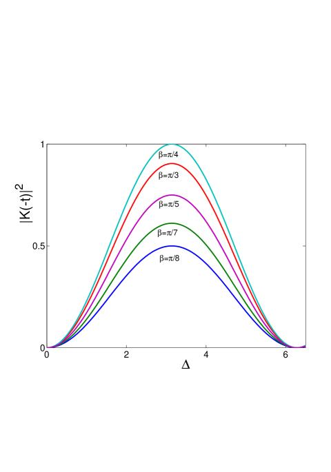
Figure 2: Parameter $|K(-t)|^{2}$ changes with time-dependent variable $\Delta=t\,\delta$ for different $\beta$ values.

we draw the curves of $|K(-t)|$ changing with time $t$ for different parameters $\beta$. For $\beta=\pi/4$, one can easily see that $|K(-t)|$ can reach unity while $|F_{k}(-t)|$ vanishes. This implies that a perfect exchange of quantum states can be implemented between the NAMR and the TRL. Mathematically, when $\beta=\pi/4,\,F_{k}(t)$ and $K(t)$ define two complementary oscillations with amplitudes ranging from $0$ to $1$. The simple amplitude complementary relation

$$|F_{k}(t)|^{2}+|K(t)|^{2}=1$$ (11)

and the same phase factor means a perfect transfer of quantum states. Physically, $\beta=\pi/4$ means that the effective couplings $\lambda_{a}$ and $\lambda_{b}$, of the NAMR and the TLR, are the same. Indeed, we can realize the perfect transfer of quantum information at the moments $t=(2m+1)/\delta$ for $a(-t)=b(0)\exp(i\omega_{a}t)$, i.e., the wave function can be factorized into

$$\sum c_{n}|n\rangle\otimes|0\rangle\rightarrow W\sum c_{n}|0\rangle\otimes|n\rangle$$

by a known unitary transformation

$$W={\rm diag}\,\{\exp(i\omega_{a}t),\exp(i2\omega_{a}t),...,\exp(in\omega_{a}t)\},$$

which is independent of the initial state.

IV Case II: Quantum information transfer for two non-degenerate modes

In the degenerate case we have demonstrated the perfect transmission of quantum states between the NAMR and TLR by connecting them via a charge qubit. In principle, it is also possible to perform quantum information transfer between two non-degenerate modes. In fact, the model of two non-degenerate modes coupled to a two-level system can be solved exactly, and the phenomenon of rapid-collapse and revival could be shown jmo01 . However, it is convenient to adiabatically eliminate the connecting qubit for directly transferring quantum states between the two non-degenerate modes.

Again, we assume that the large detuning condition is still satisfied. To directly connect the two non-degenerate modes by adiabatically eliminating the qubit, we introduce an anti-Hermitian operator

$$W=-i\frac{\lambda_{a}}{\Lambda}(a\sigma_{+}+a^{\dagger}\sigma_{-})-\frac{\lambda_{b}}{\Lambda}(b\sigma_{+}-b^{\dagger}\sigma_{-}),$$ (12)

to perform the Fröhlich-Nakajima transformation on $H_{2}$ and obtain the following effective Hamiltonian

$$H_{4} \simeq \omega_{a}a^{{\dagger}}a+\omega_{b}b^{{\dagger}}b+\frac{\Omega}{2}\sigma_{z}+\left(\frac{\lambda_{a}^{2}}{\Lambda}a^{\dagger}a+\frac{\lambda_{b}^{2}}{\Lambda}b^{\dagger}b\right)\sigma_{z}$$ (13)

$$+i\frac{\lambda_{a}\lambda_{b}}{\Lambda}(ab^{\dagger}-a^{\dagger}b)\sigma_{z}.$$

with $\Omega=\epsilon+(\lambda_{a}^{2}+\lambda_{b}^{2})/\Lambda$. The detuning

$$\Lambda=-\omega_{a}-\omega_{b}+\Omega$$

is set to satisfy the conditions:

$$\lambda_{a},\,\lambda_{b}\gg\Lambda.$$ (14)

The anti-Hermitian operator $W$ satisfies the condition

$$H_{2}-H_{0}+[H_{0},W]=0,\,\,\,H_{0}=\omega_{a}a^{\dagger}a+\omega_{b}b^{\dagger}b+\frac{\epsilon}{2}\sigma_{z},$$ (15)

which means that the first-order correction vanishes and the above approximation is second-order perturbation.

Without loss of generality, the charge qubit could be adiabatically fixed in the ground state $|0\rangle$. As a consequence, the dynamics of this two-boson system can be described by

$$H^{\prime}_{4}\,=\,\Gamma_{0}\,\hat{N}+\Gamma_{2}\,\hat{J}_{y}+\Gamma_{3}\,\hat{J}_{z}$$ (16)

with

$$\Gamma_{0} = \frac{\omega_{a}+\omega_{b}}{2}+\frac{\lambda_{a}^{2}+\lambda_{b}^{2}}{2\Lambda},$$

$$\Gamma_{2} = \frac{2\lambda_{a}\lambda_{b}}{\Lambda},$$

$$\Gamma_{3} = \omega_{a}-\omega_{b}+\frac{\lambda_{a}^{2}-\lambda_{b}^{2}}{\Lambda},$$

and $\hat{N}=b^{+}b+a^{+}a$. Angular momentum operators $\hat{J}_{l}\,(l=x,y,z)$, defined by the following Jordan-Schwinger realizations

$$\hat{J}_{x} = \frac{b^{+}a+a^{+}b}{2},$$

$$\hat{J}_{y} = \frac{i(b^{+}a-a^{+}b)}{2},$$ (17)

$$\hat{J}_{z} = \frac{a^{+}a-b^{+}b}{2},$$

form a dynamic $SO(3)$ algebra:

$$[\hat{J}_{z},\hat{J}_{x}]=i\hat{J}_{y},\,\,[\hat{J}_{y},\hat{J}_{z}]=i\hat{J}_{x},\,\,[\hat{J}_{x},\hat{J}_{y}]=i\hat{J}_{z}.$$ (18)

Obviously, $\hat{N}$ commutes with the operators $\hat{J}_{z}$ and $\hat{J}_{y}$. This implies that the Hamiltonian $H^{\prime}_{4}$ describes a high-spin precession in an external “magnetic field” $B=(0,\Gamma_{2},\Gamma_{3})$, and thus is exactly solvable sun-z . The corresponding time-evolution operator is

$$\hat{U}(t) = \exp(-\frac{i}{\hbar}\Gamma_{0}\,\hat{N}t)\,\exp(-\frac{i}{\hbar}\tilde{H}t),$$

$$\tilde{H} = \tilde{\Gamma}\exp(i\beta\,\hat{J}_{x})\,\hat{J}_{z}\,\exp(-i\beta\,\hat{J}_{x}),$$ (19)

with $\tilde{\Gamma}=\sqrt{\Gamma_{2}^{2}+\Gamma_{3}^{2}}$, and $\tan\beta=\Gamma_{2}/\Gamma_{3}$.

The above dynamics can be used to achieve the transfer of an arbitrary quantum state between the two non-degenerate modes. As a simple example, we discuss how to transfer a single-phonon state $|1_{b}\rangle$ from the NAMR to the TLR, whose initial state is the vacuum state $|0_{a}\rangle$. The initial state of this two-mode system is $|\psi(0)\rangle=|0_{a},1_{b}\rangle$. The wave function at time $t$ reads

$$|\psi(t)\rangle = \hat{U}(t)\,|\psi(0)\rangle$$ (20)

$$= \left[\cos\left(\frac{\tilde{\Gamma\,t}}{2\hbar}\right)+i\cos\beta\sin\left(\frac{\tilde{\Gamma\,t}}{2\hbar}\right)\right]|0_{a},1_{b}\rangle$$

$$- \sin\beta\sin\left(\frac{\tilde{\Gamma\,t}}{2\hbar}\right)|1_{a},0_{b}\rangle.$$

If $\Gamma_{3}=0$, a perfect transfer of quantum information is obtained by setting the duration as $\sin[\tilde{\Gamma t}/(2\hbar)]=\pm 1$. For the generic case, $\Gamma_{3}\neq 0$, a projective measurement $\hat{P}_{b}=|0_{b}\rangle\langle 0_{b}|$ acting on the NAMR is required for projecting the TLR collapse to the desirable state $|1_{a}\rangle$. The rate of this transfer is

$$P(t)=\sin^{2}\beta\sin^{2}\left(\frac{\tilde{\Gamma\,t}}{2\hbar}\right),$$ (21)

with the maximal value $\sin^{2}\beta$ corresponding to the duration $\sin[\tilde{\Gamma t}/(2\hbar)]=\pm 1$.

V Quasi–classical state of the Nano-mechanical resonator

Above, we have discussed how to transfer a quantum state from the NAMR to the TLR. Now, we investigate the preparation of a quasi-classical state of the NAMR, driven by a classical current input from the TLR. Adiabatically eliminating the connecting qubit results in an indirectly coupling between the TLR and the NAMR. Via such a virtual process, the current in TLR produces an effective linear force acting on the NAMR mode. This force causes a quasi-classical deformation of the NAMR. Therefore, a coherent state, which is described by a displaced Gaussian wave packet in the spatial position, can be generated in the NAMR mode.

For this goal, we treat the driving current classically by the Bogliubov approximation, that replaces the above annihilation and creation operators $a$ and $a^{{\dagger}}$ by the complex amplitudes $\xi=\mu\exp[-i\varphi]$ and $\xi^{*}=\mu\exp[i\varphi]$ respectively, where the real numbers $\mu$ and $\varphi$ are the amplitude and phase of the classical current, respectively. We assume, like in the previous section, that the large detuning condition is still satisfied. Thus, one can adiabatically eliminate the connected qubit and obtain a semi-classical Hamiltonian

$$H_{e}=\Omega_{b}b^{{\dagger}}b+i\frac{\Gamma_{2}}{2}\mu(e^{-i\varphi}b^{{\dagger}}-be^{i\varphi}),$$ (22)

with $\Omega_{b}=\omega_{b}+\lambda_{b}^{2}/\Lambda$. This Hamiltonian drives the NAMR to evolve from a vacuum state $|0\rangle$ to the coherent state

$$|z(t)\rangle=\exp[-|z(t)|^{2}]\,\sum_{n=0}\frac{[z(t)]^{n}}{\sqrt{n!}}|n\rangle,$$ (23)

with

$$z(t)=-i\frac{\Gamma_{2}\,\xi}{2\,\Omega_{b}}[1-\exp(-i\Omega_{b}\,t/\hbar)].$$

The above coherent state (23) corresponds to a coherent oscillation in a normal mode of the NAMR. The square of the coherent state amplitude represents the population rate of the boson excitation in the transmission line.

To this end, we require a classical TLR current in a single mode, which plays a similar role as the classical pump laser in optical masers. While switching on the coupling with the off-resonance charge qubit for a while, the charge qubit results in a virtual process as an effective linear force on a NAMR mode. It thus causes a quasi-classical deformation of the NAMR, described by a coherent state, which is a displaced Gaussian wave packet in the spatial position. This physical mechanism is very similar to that of the pulsed atomic laser BEC .

Even without adiabatic elimination for large detuning, we can still achieve the same qualitative conclusion for the state preparation. In the two cases: (a) $\omega_{b}=\epsilon$, and (b) $\omega_{a}=\omega_{b}$, the achieved semi-classical Hamiltonian

$$H_{c}=\frac{\epsilon}{2}\sigma_{z}+\omega_{b}b^{\dagger}b+[(\lambda_{b}b+i\lambda_{a}\xi)\sigma_{+}+h.c]$$ (24)

describes a driven Jaynes-Commings model. Now, we can uniquely deal with both cases as follows. If we define the displaced boson operator

$$B^{\prime}=b+i\lambda_{a}\xi,$$

$H_{c}$ becomes the standard Jaynes-Commings Hamiltonian with interaction $\lambda_{b}(B^{\prime}\sigma_{+}+h.c)$, but its ground state experiences a symmetry-breaking. Let $|n(z)\rangle=D(-z)|n\rangle$ be the displaced Fock state defined by the coherent state generator $D(z)=\exp(zb^{{\dagger}}-z^{\ast}b).$ The ground state of the NAMR-CPB composite system is just a product state $|\alpha=i\lambda_{a}\xi\rangle\otimes|g\rangle$, basically consisting of a coherent state of the NAMR. This simple observation reveals that the charge-qubit-based preparation of the quasi-classical state of the NAMR is robust.

VI Concluding remarks

In summary, we propose a mechanism to interface a transmission line resonator (TLR) with a nano-mechanical resonator (NAMR) by commonly coupling them to a charge qubit, a Cooper pair box with a controllable gate voltage. Integrated in this quantum transducer or simple quantum network, the charge qubit plays the role of a controllable quantum node coherently exchanging quantum information between the boson modes of the TLR and NAMR. We have shown that quantum information can be transferred between these two, both degenerate and non-degenerate, boson modes. Also, with such an interface, a quasi-classical state of the NAMR can be created by controlling a single-mode classical current in the TLR. Alternatively, a “Cooper pair” coherent output through the transmission line can be driven by a single-mode classical oscillation of the NAMR.

This work was supported in part by the National Security Agency (NSA) and Advanced Research and Development Activity (ARDA) under Air Force Office of Research (AFOSR) contract number F49620-02-1-0334, and by the National Science Foundation grant No. EIA-0130383. The work of C.P.S is also partially supported by the NSFC, and FRPC with No. 2001CB309310.

References

- (1) see, e.g., D.P. DiVincenzo, Fortsch. Phys. 48, 771 (2000).
- (2) X.M.H. Huang, C.A. Zorman, M. Mehregany, and M.L. Roukes, Nature (London) 421, 496 (2003).
- (3) R.G. Knobel and A.N. Cleland, Nature 424, 291 (2003).
- (4) M.D. LaHaye, O. Buu, B. Camarota, K.C. Schwab, Science 304, 74 (2004).
- (5) A. Hopkins, K. Jacobs, S. Habib and K. Schwab, Phys. Rev. B 68, 235328 (2003); E.K. Irish and K. Schwab, ibid. 68, 155311 (2003).
- (6) I. Martin, A. Shnirman, L. Tian, and P. Zoller, Phys. Rev. B 69, 125339 (2004); P. Rabl, A. Shnirman, and P. Zoller, ibid. 70, 205304 (2004); A. Gaidarzhy, G. Zolfagharkhani, R.L. Badzey, and P. Mohanty, Phys. Rev. Lett. 94, 030402 (2005).
- (7) A. Blais, R.-S. Huang, A. Wallraff, S.M. Girvin, and R.J. Schoelkopf, Phys. Rev. A 69, 062320 (2004).
- (8) A.D. Armour, M.P. Blencowe, and K.C. Schwab, Phys. Rev. Lett. 88, 148301 (2002).
- (9) A.N. Cleland and M.R. Geller, Phys. Rev. Lett. 93, 070501 (2004).
- (10) Y.D. Wang, Y.B. Gao, C.P. Sun, Euro. Phys. J. B 40, 321 (2004).
- (11) A. Wallraff, D.I. Schuster, A. Blais, L. Frunzio, R.S. Huang, J. Majer, S. Kumar, S.M. Girvin, R.J. Schoelkopf, Nature 431, 162 (2004).
- (12) J.Q. You, S.J. Tsai, and F. Nori, Phys. Rev. Lett. 89, 197902 (2002); Yu-xi Liu, L.F. Wei, and F. Nori, Phys. Rev. A 71, 063820 (2005); L.F. Wei, Yu-xi Liu, and F. Nori, arXiv: quant-ph/0408089; Phys. Rev. B (in press).
- (13) J.Q. You and F. Nori, Phys. Rev. B 68, 064509 (2003); J. Q. You, J. S. Tsai, and F. Nori, Phys. Rev. B 68, 024510 (2003); Yu-xi Liu, L.F. Wei, and F. Nori, Europhys. Lett. 67, 941 (2004); Phys. Rev. B 72, 014547 (2005).
- (14) A. Blais, A. M. van den Brink, and A. M. Zagoskin, Phys. Rev. Lett. 90, 127901 (2003); L.F. Wei, Yu-xi Liu, and F. Nori, Europhys. Lett. 67, 1004 (2004); Phys. Rev. B 71, 134506 (2005).
- (15) L. Tian, P. Rabl, R. Blatt, and P. Zoller, Phys. Rev. Lett. 92, 247902 (2004).
- (16) L. Tian and P. Zoller, Phys. Rev. Lett. 93, 266403 (2004).
- (17) A.S. Sorensen, C.H. van der Wal, L.I. Childress, and M.D. Lukin, Phys. Rev. Lett. 92, 063601 (2004).
- (18) S. Scheider, A.M. Herkommer, U. Leonhardt, and W.P. Schleich, J. Mod. Opt. 44, 2333 (1997).
- (19) G. Benivegna, and A. Messina, J. Mod. Opt. 41, 907 (1994).
- (20) Y.B. Xie, J. Mod. Opt. 42, 2239 (1994).
- (21) H. Fröhlich, Phys. Rev. 79, 845 (1950).
- (22) S. Nakajima, Adv. Phys. 4, 463 (1953).
- (23) C.P. Sun, Y.B. Gao, H.F. Dong, and S.R. Zhao, Phys. Rev. E 57, 3900 (1998).
- (24) See, e.g., A. Messina, S. Maniscalco, and A. Napoli, J. Mod. Opt. 50, 1 (2003).
- (25) C.P. Sun and L.Z. Zhang, Physica Scripta, 51, 16 (1995).
- (26) M.-O. Mewes, M.R. Andrews, D.M. Kurn, D.S. Durfee, C.G. Townsend, and W. Ketterle, Phys. Rev. Lett. 78, 582 (1997).