Strong-field approximation for intense-laser atom processes: the choice of gauge

Abstract

The strong-field approximation can be and has been applied in both length gauge and velocity gauge with quantitatively conflicting answers. For ionization of negative ions with a ground state of odd parity, the predictions of the two gauges differ qualitatively: in the envelope of the angular-resolved energy spectrum, dips in one gauge correspond to humps in the other. We show that the length-gauge SFA matches the exact numerical solution of the time-dependent Schrödinger equation.

Quantum mechanics is gauge invariant: it is easily proven that a given physical quantity can be evaluated in any gauge with the same result ct . In nonrelativistic quantum mechanics, when the dipole approximation is adopted, the interaction of an atom with a time-dependent field such as a laser field is usually described in either one of two gauges: the length gauge (L gauge) or the velocity gauge (V gauge). In numerical solutions of the time-dependent Schrödinger equation (TDSE), gauge invariance has been confirmed many times. In analytical work, however, some approximations almost always have to be adopted. There is no formal reason of why after such approximations the resulting theory should still be gauge invariant. Indeed, the lack of gauge invariance after what seems like very well justified approximations has driven many a researcher to despair jaynes .

In this paper, we will address one of the most glaring manifestations of this “gauge problem”: the lack of gauge invariance of the strong-field approximation (SFA) in intense-laser–atom physics KFR . The SFA underlies almost any analytical approach to total ionization rates, above-threshold ionization, high-order harmonic generation, and nonsequential double ionization, both of atoms and of molecules. Briefly, it assumes that the initial bound state of the atom or molecule is unaffected by the laser field while the final state, which is in the continuum, does not feel the presence of the binding potential. The lack of gauge invariance of the SFA has been noted many times; see, e.g., Ref. SBBS . Comparisons that have been carried out indeed have exhibited significant disagreements between the results obtained from L gauge and V gauge palermo . Different authors have preferred different gauges. The question of which gauge is superior for which problem has often been raised, but never led to any consensus about its answer. Below, we will give an answer for the case of a short-range binding potential, where the SFA is expected to be most accurate GK , by comparing the SFA in L gauge and V gauge with the numerical solution of the TDSE.

For a fixed nucleus and in the single-active-electron approximation, where the effects of all electrons but one are absorbed into an effective binding potential, the complete Hamiltonian in the presence of an external electromagnetic field can be decomposed as

$$H_{x}(t)=H_{0}+H_{\mathrm{I}x}(t),$$ (1)

where the subscript $x$ specifies the gauge ($x=\mathrm{L},\mathrm{V}$) and

$$H_{0}=\frac{\hat{\mathbf{p}}^{2}}{2m}+V(\mathbf{r})\ \ \mathrm{with}\ \ \hat{\mathbf{p}}=-i\mbox{\boldmath{$\nabla$}}.$$ (2)

This operator contains the binding potential $V(\mathbf{r})$ and is independent of the gauge. With the dipole approximation, which neglects the space dependence of the electric field and the vector potential, so that $\mathbf{E}(\mathbf{r},t)\rightarrow\mathbf{E}(t)$ and $\mathbf{A}(\mathbf{r},t)\rightarrow\mathbf{A}(t)$, respectively, the electron-field interaction operator has the following forms in length gauge and velocity gauge:

$$H_{\mathrm{I}x}(t)=\left\{\begin{array}[]{l}-e\mathbf{r}\cdot\mathbf{E}(t),\ (x=\mathrm{L})\\ -\frac{e}{m}\hat{\mathbf{p}}\cdot\mathbf{A}(t)+\frac{e^{2}}{2m}\mathbf{A}^{2}(t).\ (x=\mathrm{V})\end{array}\right.$$ (3)

A free electron (no binding potential) in the presence of the laser field is governed by the Hamiltonian

$$H_{\mathrm{F}x}(t)=\frac{\hat{\mathbf{p}}^{2}}{2m}+H_{\mathrm{I}x}(t).$$ (4)

The time-evolution operator of the total Hamiltonian (1) satisfies the Dyson equation

$$U_{x}(t,t^{\prime})=U_{0}(t,t^{\prime})-i\int\limits^{t}_{t^{\prime}}d\tau\,U_{x}(t,\tau)H_{\mathrm{I}x}(\tau)U_{0}(\tau,t^{\prime}),$$ (5)

where $U_{0}(t,t^{\prime})$ denotes the time-evolution operator of the Hamiltonian (2).

The exact ionization amplitude from an initial bound state $|\psi_{0}(t)\rangle=|0\rangle\exp(iI_{\mathrm{p}}t)$ with ionization potential $I_{\mathrm{p}}$ to a final continuum state $|\psi_{\mathbf{p}}(t)\rangle$, both defined by the Hamiltonian $H_{0}$, is

$$M_{\mathbf{p}}=\lim_{t\to\infty,t^{\prime}\to-\infty}\langle\psi_{\mathbf{p}}(t)|U_{x}(t,t^{\prime})|\psi_{0}(t^{\prime})\rangle.$$ (6)

We assume that the laser field be turned off in the limits of $t\rightarrow\infty$ and $t^{\prime}\rightarrow-\infty$ and that $\mathbf{A}(\infty)=\mathbf{A}(-\infty)=\mathbf{0}$. Gauge invariance then implies that $M_{\mathbf{p}}$ be gauge invariant, and indeed this can easily be verified explicitly. The SFA is obtained if we insert the Dyson equation (5) into the ionization amplitude (6). The first term, which comes from $U_{0}(t,t^{\prime})$, cancels since the initial and the final state are orthogonal, and we are left with advances

$$M_{\mathbf{p}}=-i\lim_{t\to\infty}\int^{t}_{-\infty}d\tau\langle\psi_{\mathbf{p}}(t)|U_{x}(t,\tau)H_{\mathrm{I}x}(\tau)|\psi_{0}(\tau)\rangle,$$ (7)

which is still exact.

In the argument that follows we restrict ourselves for the sake of transparence and simplicity to “direct” electrons, i.e., those that after the initial ionization never again feel the binding potential. In order to obtain the transition amplitude for the direct electrons, we replace in Eq. (7) the exact state at time $\tau$, which is $\langle\psi_{\mathbf{p}}(t)|U_{x}(t,\tau)$, by the Volkov state $\langle\psi^{(\mathrm{Vv})}_{\mathbf{p}x}(\tau)|$ [given below in Eq. (9)] where the interaction with the binding potential is neglected. This yields the well-known SFA amplitude KFR

$$M_{\mathbf{p}}=-i\int^{\infty}_{-\infty}d\tau\langle\psi^{(\mathrm{Vv})}_{\mathbf{p}x}(\tau)|H_{\mathrm{I}x}(\tau)|\psi_{0}(\tau)\rangle.$$ (8)

Here, for times $t<\tau$ the state of the electron is governed by the Hamiltonian $H_{0}$, while for $t>\tau$ its time evolution follows the Hamiltonian $H_{\mathrm{F}x}$.

The matrix element (8) conveys the following physical picture: for times $t<\tau$ the electron is sufficiently deeply bound that to a good approximation its interaction with the laser field can be ignored. At time $\tau$, it is ionized, and the laser intensity is high enough to move the electron so rapidly out of the range of the binding potential that now the latter can be neglected.

However, this physical picture is in agreement with the formal description only within L gauge. In L gauge, the interaction with the laser field is accomplished by the scalar potential $e\Phi(t)=H_{\mathrm{IL}}(t)$. There is no vector potential, so that the operator of the velocity is $\hat{\mathbf{v}}=\mathbf{p}/m$. Hence, $\hat{\mathbf{p}}^{2}/(2m)$ is the operator of the kinetic energy, and $H_{0}$ describes an atom that does not interact with the field, even if a field is present. In V gauge, the operator of the velocity is $\hat{\mathbf{v}}=[\hat{\mathbf{p}}-e\mathbf{A}(t)]/m$ where $\hat{\mathbf{p}}$ is the operator of the canonical momentum. This is a conserved quantity under the dipole approximation, but not a physical quantity ct , since $\hat{\mathbf{p}}=m\hat{\mathbf{v}}+e\mathbf{A}(t)$, and $\hat{\mathbf{v}}$ is a physical quantity while $\mathbf{A}(t)$ is not. In consequence, in the presence of a laser field, the operator $H_{0}$ is not the field-free Hamiltonian, and its eigenstate $|\psi_{0}(t_{0})\rangle$ does incorporate some interaction with the field footnote1 . Hence, in V gauge, the physical picture formulated above is not supported by the matrix element (8).

It is instructive to evaluate the matrix element (8) by the method of steepest descent, which is known to work very well for sufficiently high intensity. We first recall the explicit form of the Volkov wave function

$$\langle\mathbf{r}|\psi^{(\mathrm{Vv})}_{\mathbf{p}x}(t)\rangle=\frac{e^{-iS_{\mathbf{p}}(t)}}{(2\pi)^{\frac{3}{2}}}\left\{\begin{array}[]{l}e^{i\mathbf{p}\cdot\mathbf{r}},\ \ (x=\mathrm{V})\\ e^{i(\mathbf{p}-e\mathbf{A}(t))\cdot\mathbf{r}},\ (x=\mathrm{L})\end{array}\right.$$ (9)

with the action

$$S_{\mathbf{p}}(t)=\frac{1}{2m}\int^{t}d\tau(\mathbf{p}-e\mathbf{A}(\tau))^{2}.$$ (10)

which has the same form in either gauge footnote .

Via an integration by parts, the transition amplitude (8) can be recast in the form advances

$$M_{\mathbf{p}}=-i\int^{\infty}_{-\infty}d\tau\langle\psi^{(\mathrm{Vv})}_{\mathbf{p}x}(\tau)|V(\mathbf{r})|\psi_{0}(\tau)\rangle,$$ (11)

which depends on the gauge only via the Volkov wave function (9). Collecting the exponential time dependence of the integrand in Eq. (11) we find that the stationary points with respect to $\tau$ are determined as the solutions of the saddle-point equation

$$[\mathbf{p}-e\mathbf{A}(\tau)]^{2}=-2mI_{\mathrm{p}}.$$ (12)

The transition amplitude then can be represented as the superposition of the contributions of all those solutions $t_{s}$ of Eq. (12) for which $\mathrm{Im}t_{s}>0$, with the result

$$M_{\mathbf{p}}=\sum_{s}V_{\mathbf{p}xs}\sqrt{\frac{2\pi i}{\mathbf{E}(t_{s})\cdot[\mathbf{p}-e\mathbf{A}(t_{s})]}}e^{i[S_{\mathbf{p}}(t_{s})+I_{\mathrm{p}}t_{s}]}.$$ (13)

Only the form factor

$$V_{\mathbf{p}xs}=\left\{\begin{array}[]{l}\langle\mathbf{p}|V(\mathbf{r})|0\rangle,\ \ (x=\mathrm{V}),\\ \langle\mathbf{p}-e\mathbf{A}(t_{s})|V(\mathbf{r})|0\rangle,\ \ (x=\mathrm{L})\end{array}\right.$$ (14)

depends on the gauge. In V gauge, it is evaluated at the momentum $\mathbf{p}$ at the detector, which is the same for all saddle-point solutions. In L gauge, it is evaluated at the instantaneous velocity at the ionization time $t_{s}$, whose component parallel to the laser field according to Eq. (12) is purely imaginary and can have either sign. For a monochromatic linearly polarized laser field, there are two solutions $t_{s}$ per cycle of the saddle-point equation (12) with $\mathrm{Im}t_{s}>0$, one on either side of the pertinent extremum of the vector potential.

To find out the signs of $\mathbf{p}-e\mathbf{A}(t_{s})$ that correspond to the solutions with $\mathrm{Im}t_{s}>0$, let us consider the vector potential $\mathbf{A}(t)=\mathbf{e}A\cos\omega t$. We let $t=t_{\mathrm{R}}+it_{\mathrm{I}}$, where $t_{\mathrm{R}}$ and $t_{\mathrm{I}}$ denote the real and the imaginary part of $t$, respectively. The real and imaginary parts of the saddle-point equation (12) are

$$p_{\parallel}-eA\cos\omega t_{\mathrm{R}}\cosh\omega t_{\mathrm{I}}=0,$$ (15a)

$$eA\sin\omega t_{\mathrm{R}}\sinh\omega t_{\mathrm{I}}=\sqrt{2mI_{\mathrm{p}}+\mathbf{p}_{\perp}^{2}},$$ (15b)

where $p_{\parallel}$ and $\mathbf{p}_{\perp}$ are the components of $\mathbf{p}$ parallel and perpendicular to the laser field and the square root may have either sign. From Eq. (15a), the two solutions per cycle are such that $\cos\omega t_{\mathrm{R}}$ has the same sign. Then, from Eq. (15b) and the fact that $t_{\mathrm{I}}>0$ for the physical saddle-point solutions, we have that $\sin\omega t_{\mathrm{R}}$ has the opposite sign for the two solutions. Hence, the two instantaneous velocities that enter the L-gauge form factor (14) are $\mathbf{p}-e\mathbf{A}(t_{s})=(\pm i\sqrt{2mI_{\mathrm{p}}+\mathbf{p}_{\perp}^{2}},\mathbf{p}_{\perp})$. For $\mathbf{p}_{\perp}=\mathbf{0}$, they are purely imaginary and have opposite sign. This reflects the fact that the electric field $\mathbf{E}(t_{\mathrm{R}})$ points in opposite direction for the two solutions.

Now, for an even-parity ground state $|0\rangle$, $\langle-\mathbf{a}|V|0\rangle=\langle\mathbf{a}|V|0\rangle$, while for an odd-parity state $\langle-\mathbf{a}|V|0\rangle=-\langle\mathbf{a}|V|0\rangle$. Hence, for an odd-parity state, when in Eq. (13) the contributions of the two saddle points add in V gauge, they substract in L gauge, and vice versa. Consequently, for an odd-parity initial state, constructive interference in L gauge implies destructive interference in V gauge, and vice versa. In contrast, for an even-parity ground state, both gauges predict interference maxima and minima at the same positions. As soon as $\mathbf{p}_{\perp}\neq 0$, there is no complete destructive or constructive interference anymore.

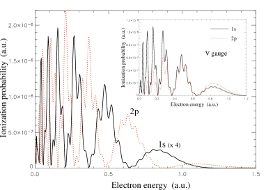
Figure 1: (color online) SFA electron energy spectrum for emission in the (positive) direction of the laser field (four-cycle $\sin^{2}$-pulse with $\phi=0$, $\omega=0.056$  a.u., $E_{0}=0.0834$ a.u.) in L gauge, starting from an initial 1s (solid) or 2p (dashed) state. The corresponding V gauge result is shown in the inset.

In Figs. 1, 2, and 3 we compare the results of the SFA in L gauge and V gauge with a numerical solution of the TDSE. All calculations have been carried out for a 4-cycle linearly polarized laser pulse having the intensity $2.4\times 10^{14}\;\mathrm{W/cm}^{2}$ (field strength $E_{0}=$ 0.0834 a.u.), and wavelength 800 nm (photon energy $\omega=$ 0.056 a.u.). The electric-field vector is $E(t)\cos(\omega t+\phi)\hat{\mathbf{e}}$, with the sine-square envelope $E(t)=E_{0}\sin^{2}\frac{\omega t}{2n_{\mathrm{p}}}$ for $0\leq t\leq T_{\mathrm{p}}=n_{\mathrm{p}}T$, $T=2\pi/\omega$, and $E(t)=0$ outside this interval. The carrier-envelope phase is $\phi=0$. Figure 1 exhibits the results of a numerical computation (not using the saddle-point approximation) of the SFA amplitude (8) in L gauge and V gauge, respectively, taking for $|\psi_{0}(t)\rangle$ the bound state of a zero-range potential GK ; MGB03 ; GMB04 ; footnote2 . They illustrate the above statements. In other words, in L gauge, everything else being equal, the positions of the interference dips for a $p$ ground state coincide with those of the interference humps for an $s$ ground state. In contrast, in V gauge dips and humps occur at the same positions regardless of the parity of the ground state. Figure 2 presents the corresponding TDSE spectrum calculated by methods introduced elsewhere DB05 . In order to mimic a short-range potential in the TDSE calculations, the Coulomb potential $-Z_{\mbox{\scriptsize eff}}/r$ has been cut at $r_{\mathrm{c}}=2$ a.u. The nuclear charge $Z_{\mbox{\scriptsize eff}}$ was adjusted in such a way as to keep the ionization potential $I_{\mathrm{p}}$ at $0.5$  a.u. for both the $1s$ and the $2p$ state. It has been shown recently DBJMO that the agreement between SFA and TDSE low-energy electron spectra improves with decreasing potential range $r_{\mathrm{c}}$. A direct comparison of the TDSE and SFA (L gauge) results is presented in Fig. 3. The agreement with respect to the energetic positions of the various peaks is excellent. Residual discrepancies are observed in the shape of the spectrum for low energies, especially for the $p$ ground state, and are likely due to the different large-distance behavior of the wave functions (zero range for the SFA vs. cut Coulomb for the TDSE).

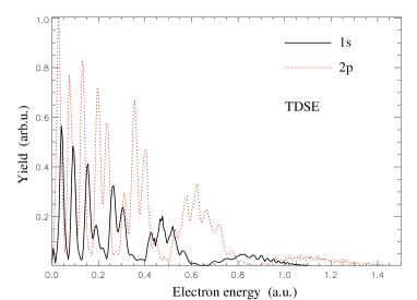
Figure 2: (color online) Same as Fig. 1, but computed from the numerical solution of the TDSE.

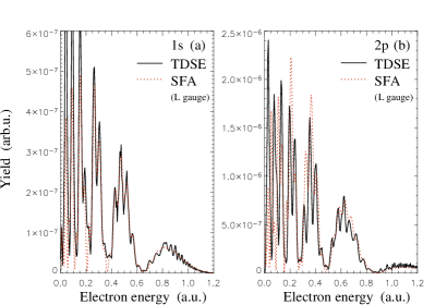
Figure 3: (color online) Direct comparison of TDSE and SFA (L gauge) photoelectron spectra. The initial states are (a) $1s$ and (b) $2p$, the other parameters as in Fig. 1. For convenience, the TDSE spectra are rescaled (but unshifted in energy).

The exact solution for ionization of negatively charged ions that is available in the context of effective-range theory exhibits the interference dips in complementary positions for $s$ and $p$ ground states manakov , in agreement with the L-gauge SFA and the exact TDSE solution. The L-gauge SFA also appears to be supported by the experimental data: the above-threshold-detachment energy spectrum for the negative F^- ion KH03 , which has a $p$ ground state, displays a pronounced change of its slope at the energy where the L-gauge SFA predicts an interference dip MGB03 ; GMB04 .

For elliptical polarization, for ellipticities higher than a certain critical value the saddle-point equation (12) only has one solution per cycle rather than two, so that the interference ceases to exist PZWLBK . This is so, in particular, for circular polarization. Recently, the latter case was considered in detail kiyan . Even in the absence of interference, the form factor (14) is still different in L gauge and in V gauge. For an $s$ ground state $|0\rangle$, the form factor $\langle\mathbf{p}|V|0\rangle$ has a maximum for $\mathbf{p}=\mathbf{0}$ and decreases with increasing $|\mathbf{p}|$, while for a $p$ state, it has a zero at $\mathbf{p}=\mathbf{0}$ and extrema away from $\mathbf{p}=\mathbf{0}$. In Ref. kiyan , for ionization of F^- by a circularly polarized laser field, the energy spectrum was calculated in either gauge. The V-gauge spectrum peaks at a higher energy than the L-gauge spectrum, which conforms with the considerations given above. Moreover, Wigner’s threshold law is only reproduced in L gauge kiyan .

Before concluding, we recall that in a numerical solution of the TDSE the choice of gauge is “merely” a question of convenience. Generally, convergence is faster in V gauge where fewer angular momenta contribute, much faster indeed for high intensity and low frequency CL . In contrast, in approximations such as the SFA, the choice of gauge is a contributing factor for the quality of the approximation. In fact, making formally the same approximation in two gauges may correspond to different approximations physically. A general argument in favor of the L gauge for use in the SFA has been put forward in Ref. GK : the L-gauge interaction Hamiltonian (3) puts the emphasis on large distances from the atom, where the Volkov wave function is a good approximation to the final state. In a similar vein, we add that it appears to make more sense to evaluate the form factor (14) at the instantaneous velocity at the time of ionization (as in L gauge) rather than at the drift velocity (as in V gauge), which for low frequencies the electron does not assume before it is far away from the ion.

On the basis of a comparison with the solution of the time-dependent Schrödinger equation, we conclude that the strong-field approximation applied to above-threshold detachment of negative ions affords a better description in length gauge than in velocity gauge. In view of the fundamental significance of the SFA for strong-field physics, it is of great importance to find out which gauge is better suited for above-threshold ionization of atoms and molecules as well as nonsequential double ionization. In all of these cases, the two gauges are known to yield different answers as well.

We enjoyed discussions with M. Yu. Ivanov, H. G. Muller, and H. R. Reiss. This work was supported by VolkswagenStiftung, Deutsche Forschungsgemeinschaft, and the NSERC Special Opportunity Program of Canada.

References

- (1) C. Cohen-Tannoudji, B. Diu, and C. Laloë, Quantum Mechanics, (Hermann/Wiley, Paris, 1977).
- (2) See, e.g., an often-quoted statement by E. T. Jaynes, communicated by D. H. Kobe and A. L. Smirl, Am. J. Phys. 46, 624 (1978).
- (3) L. V. Keldysh, Sov. Phys. JETP 20, 1307 (1964); F. H. M. Faisal, J. Phys. B 6, L89 (1973); H. R. Reiss, Phys. Rev. A 22, 1786 (1980).
- (4) R. R. Schlicher, W. Becker, J. Bergou, and M. O. Scully, in Quantum Electrodynamics and Quantum Optics, ed. by A. O. Barut, NATO ASI Series B: Physics, Vol. 10, (Plenum, New York, 1984), p. 405.
- (5) R. Burlon, C. Leone, F. Trombetta, and G. Ferrante, Nuovo Cimento 9D, 1033 (1987).
- (6) G. F. Gribakin and M. Yu. Kuchiev, Phys. Rev. A 55, 3760 (1997).
- (7) W. Becker, F. Grasbon, R. Kopold, D. B. Milošević, G. G. Paulus, and H. Walther, Adv. At., Mol., Opt. Phys. 48, 36 (2002).
- (8) This can be seen by calculating the expectation value of the kinetic energy of the state . In V gauge, it is . We assumed an eigenstate of parity so that the cross term vanishes. Clearly, the kinetic energy depends on the field, so that cannot be a field-free state. In order to obtain a truly field-free state in V gauge, we have to transform the field-free state in L gauge to V gauge. This yields the state , which has been called the “noninteracting state in V-gauge” SBBS . If this state were substituted in the transition amplitude (11) in place of , we would retrieve the same amplitude (11) in L gauge. However, this is not what the derivation presented above between Eqs. (6) and (8) yields.
- (9) It may be irritating to see in L gauge, where the vector potential is zero, the action (10) depend on . In this case, is used as short hand for any function such that the electric field can be derived as while outside the field.
- (10) D. B. Milošević, A. Gazibegović-Busuladžić, and W. Becker, Phys. Rev. A68, 050702(R) (2003).
- (11) A. Gazibegović-Busuladžić, D. B. Milošević, and W. Becker, Phys. Rev. A70, 053403 (2004).
- (12) The dependence of the SFA results on the ground-state wave function is rather weak, in particular for an ground state and L gauge. This has been checked by redoing the calculations for hydrogenic wave functions.
- (13) D. Bauer, Phys. Rev. Lett. 94, 113001 (2005).
- (14) D. Bauer, D. B. Milošević, and W. Becker, J. Mod. Opt. (submitted).
- (15) M. V. Frolov, N. L. Manakov, E. A. Pronin, and A. F. Starace, Phys. Rev. Lett. 91, 053003 (2003); J. Phys. B 36, L419 (2003).
- (16) I. Yu. Kiyan and H. Helm, Phys. Rev. Lett. 90, 183001 (2003).
- (17) G. G. Paulus, F. Zacher, H. Walther, A. Lohr, W. Becker, and M. Kleber, Phys. Rev. Lett. 80, 484 (1998).
- (18) S. Beiser, M. Klaiber, and I. Yu. Kiyan, Phys. Rev. A70, 011402(R) (2004).
- (19) E. Cormier and P. Lambropoulos, J. Phys. B 29, 1667 (1996).