’t Hooft’s quantum determinism — path integral viewpoint

Abstract

We present a path integral formulation of ’t Hooft’s derivation of quantum from classical physics. Our approach is based on two concepts: Faddeev-Jackiw’s treatment of constrained systems and Gozzi’s path integral formulation of classical mechanics. This treatment is compared with our earlier one [quant-ph/0409021] based on Dirac-Bergmann’s method.

I Introduction

In recent years, there has been a revival of interest in the conceptual foundations of quantum mechanics. In particular, a great deal of effort has gone into the construction of deterministic theories from which quantum mechanics would emerge. Proposals in this direction are now of considerable topical interest as evidenced by various recent monographs monographs and this series of workshops elzeII .

The usual caution toward the idea of deriving quantum from classical physics is mainly based on the Bell inequalities. The fact that quantum mechanics at laboratory scales obeys these inequalities is usually taken for granted to be true at all scales. This perception persists even if such fundamental concepts as rotational symmetry or isospin — on which the Bell inequalities are based — may simply cease to exist, for instance at Planck scale. In fact, at present, no viable experiment can rule out the possibility that quantum mechanics is only the low-energy limit of some more fundamental underlying (possibly even non–local) deterministic mechanism that operates at very small scales.

An interesting deterministic route to quantum physics was recently proposed by ’t Hooft tHooft ; tHooft3 ; tHooft22 , motivated by black-hole thermodynamics and the so-called holographic principle tHooft2 ; Bousso . The main concept of ’t Hooft’s approach resides in information loss, which, when inflicted upon a deterministic system, can reduce the physical degrees of freedom so that quantum mechanics emerges. The information loss together with certain accompanying non-trivial geometric phases may explain the observed non-locality in quantum mechanics. This idea has been further developed by several authors BJK ; tHooft22 ; BJV3 ; Elze ; Halliwell:2000mv ; tHooft3 ; BJV1 , and it forms the basis also of this paper.

Our aim is to study ’t Hooft’s quantization procedure by means of path integrals, as done in our previous work BJK . However, in contrast to Ref. BJK we treat the constrained dynamics — the key element in ’t Hooft’s method — by means of the Faddeev-Jackiw technique F-J . The constrained dynamics enters into ’t Hooft’s scheme twice: first, in the classical starting Hamiltonian which is of first order in the momenta and thus singular in the Dirac-Bergmann sense Dir2 . Second, in the information loss condition that we impose to achieve quantization BJK . It is thus clear that a better understanding of ’t Hooft’s quantization scheme is closely related to a proper treatment of the involved constrained dynamics. In our previous paper BJK this has been done by means of the customary Dirac-Bergmann technique, which is often cumbersome. Here we want to point out the simplifications arising from the alternative Faddeev-Jackiw method, which allows a clearer exposition of the basic concepts.

The paper is organized as follows: In Section II we briefly discuss the main features of ’t Hooft’s scheme. By utilizing the Faddeev-Jackiw procedure we present in Section III a Lagrangian formulation of ’t Hooft’s system, which allows us to quantize it via path integrals in configuration space. It is shown that the fluctuating system produces a classical partition function. In Section IV we make contact with Gozzi’s superspace path integral formulation of classical mechanics. In Section V we introduce ’t Hooft’s constraint which accounts for information loss. This is again handled by means of Faddeev-Jackiw analysis. Central to this analysis is the fact that ’t Hooft’s condition breaks the BRST symmetry and allows to recast the classical generating functional into a form representing a genuine quantum-mechanical partition function. A final discussion is given in Section VI.

II ’t Hooft’s quantization procedure

We begin with a brief review of the main aspects of ’t Hooft’s quantization procedure tHooft22 ; tHooft3 to be used in this work. The general idea is that a simple class of classical systems can be described by means of Hilbert space techniques, although they are fully deterministic. After imposing certain constraints expressing information loss (or dissipation), one obtains quantum systems. Several simple models were given by ’t Hooft to illustrate his idea, both with discrete and continuous time.

II.1 Discrete-time version

The simplest example tHooft3 is a three-state clock universe with a cyclic deterministic evolution pictured in Fig.1.

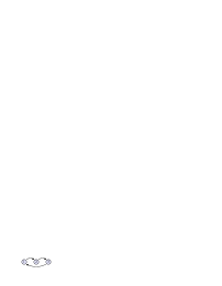
Figure 1: Three-state universe.

A Hilbert space is associated with this system consisting of the vectors tHooft3 :

$$|\psi\rangle\,=\,\alpha|1\rangle+\beta|2\rangle+\gamma|3\rangle\,.$$ (1)

At each discrete time point $t=1,2,3,4,\dots$, the system jumps cyclically. The time evolution may be represented by the unitary operator

$$|\psi\rangle_{t+1}\,=\,\left(\begin{array}[]{ccc}0&0&1\\ 1&0&0\\ 0&1&0\end{array}\right)|\psi\rangle_{t}=U(t+1,t)|\psi\rangle_{t}\,.$$ (5)

The probabilities for being in a given state are:

$$P(1)=|\alpha|^{2};\quad P(2)=|\beta|^{2};\quad P(3)=|\gamma|^{2}\,.$$ (6)

In a basis in which $U$ is diagonal, it has for a single time step $\Delta t=1$ the form:

$$U(t+1,t)=\exp(-iH\Delta t);H=\left(\begin{array}[]{ccc}0&&\\ &-2\pi/3&\\ &&2\pi/3\end{array}\right)\!.$$ (10)

A quantum theory can be said to be deterministic if, in the Heisenberg picture, a complete set of operators $O_{i}(t)$ ($i=1,..,N$) exist, such that:

$$[O_{i}(t),O_{j}(t^{\prime})]=0,\quad\forall t,t^{\prime};\quad i,j=1,..,N\,.$$ (11)

These operators are called “be-ables” tHooft3 . The above three-state system is obviously deterministic in this sense.

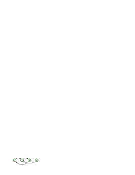
Figure 2: Four-state universe with non-unitary evolution.

It is also possible to have systems for which the evolution is not unitary, at least for a certain number of time steps tHooft3 . An example is given by the system in Fig.2 for which the time evolution generator is given by

$$U_{d}(t+1,t)\,=\,\left(\begin{array}[]{cccc}0&0&1&0\\ 1&0&0&1\\ 0&1&0&0\\ 0&0&0&0\end{array}\right)\,.$$ (16)

An important concept which arises here is that of equivalence classes tHooft3 . In our case, the states $|1)$ and $|4)$ are equivalent, in the sense that they end up in the same state after a finite time.

Quantum states are thus identified with equivalence classes:

$$|1\rangle\equiv\{|1),|4)\},\quad|2\rangle\equiv\{|2)\},\quad|3\rangle\equiv\{|3)\}\,,$$ (17)

in terms of which the time evolution becomes unitary again.

II.2 Continuous-time version

Classical systems of the form

$$H=p_{a}\,f^{a}({\mbox{\boldmath$q$\unboldmath}})\,,$$ (18)

with repeated indices summed, evolve deterministically even after quantization tHooft3 . This happens since in the Hamiltonian equations of motion

$$\dot{q}^{a} = \{q^{a},H\}=f^{a}({\mbox{\boldmath$q$\unboldmath}})\,,$$

$$\dot{p}_{a} = \{p_{a},H\}=-p_{a}\frac{\partial{f^{a}({\mbox{\boldmath$q$\unboldmath}})}}{\partial q^{a}}\,,$$ (19)

the equation for the $q^{a}$ does not contain $p^{a}$, making the $q^{a}$ be-ables. The basic physical problem with these systems is that the Hamiltonian is not bounded from below. This defect can be repaired in the following way tHooft3 : Let $\rho({\mbox{\boldmath$q$\unboldmath}})$ be some positive function of $q_{a}$ with $[\rho,H]=0$. Then we split

$$H=H_{+}-H_{-},$$

$$H_{+}=\frac{1}{4\rho}\left(\rho+H\right)^{2}\,,\quad H_{-}=\frac{1}{4\rho}\left(\rho-H\right)^{2}\,,$$ (20)

where $H_{+}$ and $H_{-}$ are positive definite operators satisfying

$$[H_{+},H_{-}]\,=\,[\rho,H]=0\,.$$ (21)

We may now enforce a lower bound upon the Hamiltonian by imposing the constraint

$$H_{-}|\psi\rangle=0\,.$$ (22)

Then the eigenvalues of $H$ in

$$H|\psi\rangle=H_{+}|\psi\rangle=\rho|\psi\rangle,$$ (23)

are trivially positive, and the equation of motion

$$\frac{d}{dt}|\psi\rangle=-iH|\psi\rangle\,,$$ (24)

has only positive frequencies. If there are stable orbits with period $T(\rho)$, then $|\psi\rangle$ satisfies

$$e^{-iHT}|\psi\rangle=|\psi\rangle\quad;\qquad\rho\,T(\rho)=2\pi n\,,\quad n\in\mathbb{Z}\,,$$ (25)

so that the associated eigenvalues are discrete. The constraint (22) was motivated by ’t Hooft by information loss tHooft3 . We shall therefore refer to it as information loss condition. Applications of the the above quantization procedure were given in Refs. BJV1 .

III Path integral quantization of ’t Hooft’s system

Consider the class of systems described by Hamiltonians of the type (18), and let us try to quantize them using path integrals PI . Because of the absence of a leading kinetic term quadratic in the momenta $p_{a}$, the system can be viewed as singular and the ensuing quantization can be achieved through some standard technique for quantization of constrained systems.

Particularly convenient technique is the one proposed by Faddeev and Jackiw F-J . There one starts by observing that a Lagrangian for ’t Hooft’s equations of motion (19) can be simply taken as

$$L({\mbox{\boldmath$q$\unboldmath}},\dot{{\mbox{\boldmath$q$\unboldmath}}},{\mbox{\boldmath$p$\unboldmath}},\dot{\mbox{\boldmath$p$\unboldmath}})~{}=\ {\mbox{\boldmath$p$\unboldmath}}\cdot\dot{\mbox{\boldmath$q$\unboldmath}}-H({\mbox{\boldmath$p$\unboldmath}},{\mbox{\boldmath$q$\unboldmath}})\,,$$ (26)

with $q$ and $p$ being Lagrangian variables (in contrast to phase space variables). Note that $L$ does not depend on $\dot{\mbox{\boldmath$p$\unboldmath}}$. It is easily verified that the Euler-Lagrange equations for the Lagrangian (26) indeed coincide with the Hamiltonian equations (19). Thus given ’t Hooft’s Hamiltonian (18) one can always construct a first-order Lagrangian (26) whose configuration space coincides with the Hamiltonian phase space. By defining $2N$ configuration-space coordinates as

$$\xi^{a}~{}=~{}p_{a},\;\;\;a=1,\ldots,N\,,$$

$$\xi^{a}~{}=~{}q^{a},\;\;\;a=N+1,\ldots,2N\,,$$ (27)

the Lagrangian (26) can be cast into the more expedient form, namely

$$L({\mbox{\boldmath$\xi$\unboldmath}},\dot{\mbox{\boldmath$\xi$\unboldmath}})~{}=~{}\mbox{$\frac{1}{2}$}\xi^{a}\omega_{ab}\dot{\xi}^{b}-H({\mbox{\boldmath$\xi$\unboldmath}})\,.$$ (28)

Here $\omega$ is the $2N\times 2N$ symplectic matrix

$${\mbox{\boldmath$\omega$\unboldmath}}_{ab}~{}=~{}\left(\begin{array}[]{ll}0&{\mbox{\boldmath$I$\unboldmath}{}}\\ -{\mbox{\boldmath$I$\unboldmath}{}}&0\end{array}\right)_{ab}\,,$$ (31)

which has an inverse ${\mbox{\boldmath$\omega$\unboldmath}}_{ab}^{-1}\equiv{\mbox{\boldmath$\omega$\unboldmath}}^{ab}$. The equations of motion read

$$\dot{\xi}^{a}~{}=~{}{\mbox{\boldmath$\omega$\unboldmath}}^{ab}\frac{\partial H({\mbox{\boldmath$\xi$\unboldmath}})}{\partial\xi^{b}}\,,$$ (32)

indicating that there are no constraints on $\xi$. Thus the Faddeev-Jackiw procedure makes the system unconstrained, so that the path integral quantization may proceeds in a standard way. The time evolution amplitude is simply PI

$$\mbox{}\langle{\mbox{\boldmath$\xi$\unboldmath}}_{2},t_{2}|{\mbox{\boldmath$\xi$\unboldmath}}_{1},t_{1}\rangle\!=\!{\mathcal{N}}\int_{\mbox{\boldmath\footnotesize$\xi$\normalsize\unboldmath}(t_{1})=\mbox{\boldmath\footnotesize$\xi$\normalsize\unboldmath}_{1}}^{\mbox{\boldmath\footnotesize$\xi$\normalsize\unboldmath}(t_{2})=\mbox{\boldmath\footnotesize$\xi$\normalsize\unboldmath}_{2}}\!{\mathcal{D}}{\mbox{\boldmath$\xi$\unboldmath}}\ \exp\left[\frac{i}{\hbar}\!\int_{t_{1}}^{t_{2}}\!dt~{}L({\mbox{\boldmath$\xi$\unboldmath}},\dot{\mbox{\boldmath$\xi$\unboldmath}})\right],$$

where ${\mathcal{N}}$ is some normalization factor, and the measure can be rewritten as

$${\mathcal{N}}\int_{\mbox{\boldmath\footnotesize$\xi$\normalsize\unboldmath}(t_{1})=\mbox{\boldmath\footnotesize$\xi$\normalsize\unboldmath}_{1}}^{\mbox{\boldmath\footnotesize$\xi$\normalsize\unboldmath}(t_{2})=\mbox{\boldmath\footnotesize$\xi$\normalsize\unboldmath}_{2}}{\mathcal{D}}{\mbox{\boldmath$\xi$\unboldmath}}={{\mathcal{N}}}\int_{{\mbox{\boldmath\footnotesize$q$\normalsize\unboldmath}}(t_{1})={\mbox{\boldmath\footnotesize$q$\normalsize\unboldmath}}_{1}}^{{\mbox{\boldmath\footnotesize$q$\normalsize\unboldmath}}(t_{2})={\mbox{\boldmath\footnotesize$q$\normalsize\unboldmath}}_{2}}{\mathcal{D}}{\mbox{\boldmath$q$\unboldmath}}{\mathcal{D}}{{\mbox{\boldmath$p$\unboldmath}}}\,.$$ (34)

Since the Lagrangian (26) is linear in $p$, we may integrate these variables out and obtain

$$\!\!\!\!\!\!\!\!\!\!\!\!\!\!\!\!\!\langle{\mbox{\boldmath$q$\unboldmath}}_{2},t_{2}|{\mbox{\boldmath$q$\unboldmath}}_{1},t_{1}\rangle={{\mathcal{N}}}\int_{{\mbox{\boldmath\footnotesize$q$\normalsize\unboldmath}}(t_{1})={\mbox{\boldmath\footnotesize$q$\normalsize\unboldmath}}_{1}}^{{\mbox{\boldmath\footnotesize$q$\normalsize\unboldmath}}(t_{2})={\mbox{\boldmath\footnotesize$q$\normalsize\unboldmath}}_{2}}{\mathcal{D}}{\mbox{\boldmath$q$\unboldmath}}~{}\prod_{a}\delta[\dot{q}^{a}-f^{a}({\mbox{\boldmath$q$\unboldmath}})]\,,$$ (35)

where $\delta[{\mbox{\boldmath$f$\unboldmath}}]\equiv\prod_{t}\delta({\mbox{\boldmath$f$\unboldmath}}(t))$ is the functional version of Dirac’s $\delta$-function. Hence the system described by the Hamiltonian (18) retains its deterministic character even after quantization. The paths are squeezed onto the classical trajectories determined by the differential equations $\dot{\mbox{\boldmath$q$\unboldmath}}={\mbox{\boldmath$f$\unboldmath}}({\mbox{\boldmath$q$\unboldmath}})$. The time evolution amplitude (35) contains a sum over only the classical trajectories — there are no quantum fluctuations driving the system away from the classical paths, which is precisely what should be expected from a deterministic dynamics.

The amplitude (35) can be brought into more intuitive form by utilizing the identity

$$\delta\left[{\mbox{\boldmath$f$\unboldmath}}({{\mbox{\boldmath$q$\unboldmath}}})-\dot{{\mbox{\boldmath$q$\unboldmath}}}\right]~{}=~{}\delta[{\mbox{\boldmath$q$\unboldmath}}-{\mbox{\boldmath$q$\unboldmath}}_{\rm cl}]~{}(\det{{M}})^{-1}\,,$$ (36)

where ${M}$ is a functional matrix formed by the second functional derivatives of the action ${{\mathcal{A}}}[{\mbox{\boldmath$\xi$\unboldmath}}]\equiv\int dt\,L({\mbox{\boldmath$\xi$\unboldmath}},\dot{\mbox{\boldmath$\xi$\unboldmath}})$ :

$${{M}}_{ab}(t,t^{\prime})~{}=~{}\left.\frac{\delta^{2}{{\mathcal{A}}}}{\delta\xi^{a}(t)~{}\delta{\xi}^{b}(t^{\prime})}~{}\right|_{{\mbox{\boldmath$q$\unboldmath}}={\mbox{\boldmath$q$\unboldmath}}_{\rm cl}}\,.$$ (37)

The Morse index theorem ensures that for sufficiently short time intervals $t_{2}-t_{1}$ (before the system reaches its first focal point), the classical solution with the initial condition ${{\mbox{\boldmath$q$\unboldmath}}}(t_{1})={\mbox{\boldmath$q$\unboldmath}}_{1}$ is unique. In such a case Eq. (35) can be brought to the form

$$\langle{\mbox{\boldmath$q$\unboldmath}}_{2},t_{2}|{\mbox{\boldmath$q$\unboldmath}}_{1},t_{1}\rangle = {\tilde{\mathcal{N}}}\int_{{\mbox{\boldmath\footnotesize$q$\normalsize\unboldmath}}(t_{1})={\mbox{\boldmath\footnotesize$q$\normalsize\unboldmath}}_{1}}^{{\mbox{\boldmath\footnotesize$q$\normalsize\unboldmath}}(t_{2})={\mbox{\boldmath\footnotesize$q$\normalsize\unboldmath}}_{2}}{\mathcal{D}}{\mbox{\boldmath$q$\unboldmath}}~{}\delta\left[{\mbox{\boldmath$q$\unboldmath}}-{\mbox{\boldmath$q$\unboldmath}}_{\rm cl}\right]\,,$$ (38)

with ${\tilde{\mathcal{N}}}\equiv{{\mathcal{N}}}/(\det{M})$. Remarkably, the Faddeev-Jackiw treatment bypasses completely the discussion of constraints, in contrast with the conventional Dirac-Bergmann method Dir2 ; Sunder where $2N$ (spurious) second-class primary constraints must be introduced to deal with ’t Hooft’s system, as done in BJK .

IV Emergent SUSY — signature of classicality

We now turn to an interesting implication of the result (38). If we had started in Eq.(35) with an external current

$$\tilde{L}({\mbox{\boldmath$\xi$\unboldmath}},\dot{\mbox{\boldmath$\xi$\unboldmath}})=L({\mbox{\boldmath$\xi$\unboldmath}},\dot{\mbox{\boldmath$\xi$\unboldmath}})+i\hbar{\mbox{\boldmath$J$\unboldmath}}\cdot{\mbox{\boldmath$q$\unboldmath}}\,,$$ (39)

integrated again over $p$, and took the trace over $q$, we would end up with a generating functional

$${\mathcal{Z}}_{\rm CM}[\mbox{\boldmath$J$\unboldmath}]=\tilde{{\mathcal{N}}}\int{\mathcal{D}}{\mbox{\boldmath$q$\unboldmath}}~{}\delta[{\mbox{\boldmath$q$\unboldmath}}-{\mbox{\boldmath$q$\unboldmath}}_{\rm cl}]\exp\left[\int_{t_{1}}^{t_{2}}dt\ {\mbox{\boldmath$J$\unboldmath}}\cdot{\mbox{\boldmath$q$\unboldmath}}\right]\,.$$ (40)

This coincides with the path integral formulation of classical mechanics postulated by Gozzi et al. GozziI ; GozziII . The same representation can be derived from the classical limit of a closed-time path integral for the transition probabilities of a quantum particle in a heat bath PI ; BJK , The path integral (40) has an interesting mathematical structure. We may rewrite it as

$${\mathcal{Z}}_{\rm CM}[\mbox{\boldmath$J$\unboldmath}]~{} = ~{}\tilde{{\mathcal{N}}}\int{\mathcal{D}}{\mbox{\boldmath$q$\unboldmath}}~{}\delta\left[\frac{\delta{{\mathcal{A}}}}{\delta{\mbox{\boldmath$q$\unboldmath}}}\right]~{}\det\left|\frac{\delta^{2}{{\mathcal{A}}}}{\delta q_{a}(t)~{}q_{b}(t^{\prime})}\right|$$ (41)

$$\times ~{}\exp\left[\int_{t_{1}}^{t_{2}}dt\ {\mbox{\boldmath$J$\unboldmath}}\cdot{\mbox{\boldmath$q$\unboldmath}}\right]\,.$$

By representing the delta functional in the usual way as a functional Fourier integral

$$\delta\left[\frac{\delta{{\mathcal{A}}}}{\delta{\mbox{\boldmath$q$\unboldmath}}}\right]=\int{\mathcal{D}}{\mbox{\boldmath$\lambda$\unboldmath}}~{}\exp\left(i\int_{t_{1}}^{t_{2}}dt~{}{\mbox{\boldmath$\lambda$\unboldmath}}(t)\frac{\delta{{\mathcal{A}}}}{\delta{\mbox{\boldmath$q$\unboldmath}}(t)}\right)\,,$$

and the functional determinant as a functional integral over two real time-dependent Grassmannian ghost variables $c_{a}(t)$ and ${\bar{c}}_{a}(t)$,

$$\det\left|\frac{\delta^{2}{\mathcal{A}}}{\delta q^{a}(t)~{}\delta q^{b}(t^{\prime})}\right|$$

$$=\int{\mathcal{D}}{\mathbf{c}}{\mathcal{D}}{\bar{{\mbox{\boldmath$c$\unboldmath}}}}~{}\exp{\left[\int_{t_{1}}^{t_{2}}dtdt^{\prime}\ \bar{c}_{a}(t)\frac{\delta^{2}{{\mathcal{A}}}}{\delta{q^{a}}(t)\ \delta{q^{b}}(t^{\prime})}~{}{c_{b}}(t^{\prime})\right]}\,,$$

we obtain

$$\mbox{}{\mathcal{Z}}_{\rm CM}[\mbox{\boldmath$J$\unboldmath}]=\int\!{\mathcal{D}}{\mbox{\boldmath$q$\unboldmath}}{\mathcal{D}}{\mbox{\boldmath$\lambda$\unboldmath}}{\mathcal{D}}{\mbox{\boldmath$c$\unboldmath}}{\mathcal{D}}\bar{{\mbox{\boldmath$c$\unboldmath}}}\exp\left[i{\mathcal{S}}+\int_{t_{1}}^{t_{2}}\!dt~{}{{\mbox{\boldmath$J$\unboldmath}}}\cdot{{\mbox{\boldmath$q$\unboldmath}}}\right]\!,$$ (42)

with the new action

$$\mbox{}{\mathcal{S}}[{\mbox{\boldmath$q$\unboldmath}},\bar{{\mbox{\boldmath$c$\unboldmath}}},{\mbox{\boldmath$c$\unboldmath}},{\mbox{\boldmath$\lambda$\unboldmath}}]\equiv~{}\int_{t_{1}}^{t_{2}}dt\ {\mbox{\boldmath$\lambda$\unboldmath}}(t)\frac{\delta{{\mathcal{A}}}}{\delta{\mbox{\boldmath$q$\unboldmath}}(t)}$$

$$\mbox{}-i\int_{t_{1}}^{t_{2}}dt\int_{t_{1}}^{t_{2}}dt^{\prime}~{}\bar{c}_{a}(t)\frac{\delta^{2}{{\mathcal{A}}}}{\delta{q^{a}}(t)~{}\delta{q^{b}}(t^{\prime})}\ {c_{b}}(t^{\prime})\,.$$ (43)

Since ${\mathcal{Z}}_{\rm CM}[\mbox{\boldmath$J$\unboldmath}]$ can be derived from the classical limit of a closed-time path integral for the transition probability, it comes to no surprise that ${\mathcal{S}}$ exhibits BRST (and anti-BRST) symmetry. It is simple to check BJK that $\mathcal{S}$ does not change under the symmetry transformations

$$\delta_{{\rm BRST\,}}{\mbox{\boldmath$q$\unboldmath}}=\bar{\varepsilon}{\mbox{\boldmath$c$\unboldmath}}\,,\;\;\;\delta_{{\rm BRST\,}}\bar{{\mbox{\boldmath$c$\unboldmath}}}=-i\bar{\varepsilon}{\mbox{\boldmath$\lambda$\unboldmath}}\,,\;\;\;\delta_{{\rm BRST\,}}{\mbox{\boldmath$c$\unboldmath}}=0\,,$$

$$\delta_{{\rm BRST\,}}{\mbox{\boldmath$\lambda$\unboldmath}}=0\,,$$ (44)

where $\bar{\varepsilon}$ is a Grassmann-valued parameter (the corresponding anti-BRST transformations are related to (44) by charge conjugation). As noted in GozziII , the ghost fields $\bar{{\mbox{\boldmath$c$\unboldmath}}}$ and $c$ are mandatory at the classical level as their rôle is to cut off the fluctuations perpendicular to the classical trajectories. On the formal side, $\bar{{\mbox{\boldmath$c$\unboldmath}}}$ and $c$ may be identified with Jacobi fields GozziII ; DeWitt . The corresponding BRST charges are related to Poincaré-Cartan integral invariants GozziIII .

By analogy with the stochastic quantization the path integral (42) can be rewritten in a compact form with the help of a superfield GozziI ; Zinn-JustinII ; PI

$$\mbox{}\Phi_{a}(t,\theta,\bar{\theta})=~{}q_{a}(t)+i\theta c_{a}(t)-i\bar{\theta}\bar{c}_{a}(t)+i\bar{\theta}\theta\lambda_{a}(t)\,,$$ (45)

in which $\theta$ and ${\bar{\theta}}$ are anticommuting coordinates extending the configuration space of $q$ variables to a superspace. The latter is nothing but the degenerate case of supersymmetric field theory in $d=1$ in the superspace formalism of Salam and Strathdee SS1 . In terms of superspace variables we see that

$$\!\!\!\!\!\!\!\!\!\!\!\int d\bar{\theta}d\theta~{}{{\mathcal{A}}}[{\mbox{\boldmath$\Phi$\unboldmath}}]$$ (46)

$$\!\!\!\!\!\!\!\!\!\!\!\!\!\!\!\!\!\mbox{\hskip 14.22636pt}=\int dtd\bar{\theta}d\theta\ L({\mbox{\boldmath$q$\unboldmath}}(t)+i\theta{\mbox{\boldmath$c$\unboldmath}}(t)-i\bar{\theta}\bar{\mbox{\boldmath$c$\unboldmath}}(t)+i\bar{\theta}\theta\mbox{\boldmath$\lambda$\unboldmath}(t))=-i{\mathcal{S}}$$

To obtain the last line we Taylor expanded $L$ and used the standard integration rules for Grassmann variables. Together with the identity ${\mathcal{D}}{\mbox{\boldmath$\Phi$\unboldmath}}={\mathcal{D}}{\mbox{\boldmath$q$\unboldmath}}{\mathcal{D}}{\mbox{\boldmath$c$\unboldmath}}{\mathcal{D}}\bar{{\mbox{\boldmath$c$\unboldmath}}}{\mathcal{D}}{\mbox{\boldmath$\lambda$\unboldmath}}$ we may therefore express the classical partition functions (40) and (41) as a supersymmetric path integral with fully fluctuating paths in superspace

$${\mathcal{Z}}_{\rm CM}[\mbox{\boldmath$J$\unboldmath}] = \int\!{\mathcal{D}}{\mbox{\boldmath$\Phi$\unboldmath}}\ \exp\left\{-\int d\theta d\bar{\theta}\ {{\mathcal{A}}}[{\mbox{\boldmath$\Phi$\unboldmath}}](\theta,\bar{\theta})\right\}$$

$$\times~{}\exp\left\{\int dtd\theta d\bar{\theta}\ {\mbox{\boldmath$\Gamma$\unboldmath}}(t,\theta,\bar{\theta}){\mbox{\boldmath$\Phi$\unboldmath}}(t,\theta,\bar{\theta})\right\}\,.$$

Here we have introduced the supercurrent ${\mbox{\boldmath$\Gamma$\unboldmath}}(t,\theta,\bar{\theta})=\bar{\theta}\theta{\mbox{\boldmath$J$\unboldmath}}(t)$.

Let us finally add that under rather general assumptions it is possible to prove BJK that ’t Hooft’s deterministic systems are the only systems with the peculiar property that their full quantum properties are classical in the Gozzi et al. sense. Among others, the latter also indicates that the Koopman-von Neumann operator formulation of classical mechanics KN1 when applied to ’t Hooft systems must agree with their canonically quantized counterparts.

V Inclusion of information loss

As observed in Section IIB, the Hamiltonian (18) is not bounded from below, and this is clearly true for any function $f^{a}({\mbox{\boldmath$q$\unboldmath}})$. Hence, no deterministic system with dynamical equations $\dot{q}^{a}=f^{a}({\mbox{\boldmath$q$\unboldmath}})$ can describe a stable quantum world. To deal with this situation we now employ ’t Hooft’s procedure of Section II.B. We assume that the system (18) has $n$ conserved irreducible charges $C^{i}$, i.e.,

$$\{C^{i},H\}=0\,,\;\;\;\;i=1,\ldots,n\,.$$ (47)

Then we enforce a lower bound upon $H$, by imposing the condition that $H_{-}$ is zero on the physically accessible part of phase space.

The splitting of $H$ into $H_{-}$ and $H_{+}$ is conserved in time provided that $\{H_{-},H\}=\{H_{+},H\}=0$, which is ensured if $\{H_{+},H_{-}\}=0$. Since the charges $C^{i}$ in (47) form an irreducible set, the Hamiltonians $H_{+}$ and $H_{-}$ must be functions of the charges and $H$ itself. There is a certain amount of flexibility in finding $H_{-}$ and $H_{+}$. For convenience take the following choice

$$H_{+}~{}=~{}\frac{(H+a_{i}C^{i})^{2}}{4a_{i}C^{i}}\,,\;\;H_{-}~{}=\ \frac{(H-a_{i}C^{i})^{2}}{4a_{i}C^{i}}\,,$$ (48)

where $a_{i}(t)$ are $q$ and $p$ independent. The lower bound is reached by choosing $a_{i}(t)C^{i}$ to be non-negative. We shall select a combination of $C^{i}$ which is $p$-independent [this condition may not necessarily be achievable for general $f^{a}({\mbox{\boldmath$q$\unboldmath}})$].

In the Dirac-Bergmann quantization approach used in our previous paper BJK , the information loss condition (22) was a first-class primary constraint. In the Dirac-Bergmann analysis, this signals the presence of a gauge freedom — the associated Lagrange multipliers cannot be determined from dynamical equations alone Dir2 . The time evolution of observable quantities, however, should not be affected by the arbitrariness of Lagrange multipliers. To remove this superfluous freedom one must choose a gauge. For details of this more complicated procedure see BJK .

In the Faddeev-Jackiw approach, Dirac’s elaborate classification of constraints to first or second class, primary or secondary is avoided. It is therefore worthwhile to rephrase the entire development of Ref. BJK once more in this approach. The information loss condition may now be introduced by simply adding to the Lagrangian (28) a term enforcing

$$H_{-}({\mbox{\boldmath$\xi$\unboldmath}})~{}=~{}0\,,$$ (49)

by means of a Lagrange multiplier:

$$L({\mbox{\boldmath$\xi$\unboldmath}},\dot{\mbox{\boldmath$\xi$\unboldmath}})=\mbox{$\frac{1}{2}$}\xi^{a}{\mbox{\boldmath$\omega$\unboldmath}}_{ab}\dot{\xi}^{b}-H({\mbox{\boldmath$\xi$\unboldmath}})-\eta H_{-}({\mbox{\boldmath$\xi$\unboldmath}})\,,$$ (50)

Alternatively, we shall eliminate one of $\xi^{a}$, say $\xi^{1}$, in terms of the remaining coordinates ones, thus reducing the dynamical variables to $2N-1$. Apart from an irrelevant total derivative, this changes the derivative term $\xi^{a}{\mbox{\boldmath$\omega$\unboldmath}}_{ab}\dot{\xi}^{b}$ to $\xi^{i}{\mbox{\boldmath$f$\unboldmath}}_{ij}(\hat{{\mbox{\boldmath$\xi$\unboldmath}}})\dot{\xi}^{j}$, with

$${\mbox{\boldmath$f$\unboldmath}}_{ij}(\hat{{\mbox{\boldmath$\xi$\unboldmath}}})=\omega_{ij}-\left[\omega_{1i}\frac{\partial\xi^{1}}{\partial\xi^{j}}-(i\leftrightarrow j)\right].$$ (51)

Eliminating $\xi^{1}$ also in the Hamiltonian $H$ we obtain a reduced Hamiltonian $H_{R}(\mbox{\boldmath$\xi$\unboldmath})$, so that we are left with a reduced Lagrangian

$$L_{R}(\hat{{\mbox{\boldmath$\xi$\unboldmath}}},\dot{\hat{\mbox{\boldmath$\xi$\unboldmath}}})~{}=\ \mbox{$\frac{1}{2}$}\xi^{i}{\mbox{\boldmath$f$\unboldmath}}_{ij}(\hat{{\mbox{\boldmath$\xi$\unboldmath}}})\dot{\xi}^{j}-H_{R}(\hat{{\mbox{\boldmath$\xi$\unboldmath}}})\,.$$ (52)

At this point one must worry about the notorious operator-ordering problem, not knowing in which temporal order $\hat{{\mbox{\boldmath$\xi$\unboldmath}}}$ and $\dot{\hat{\mbox{\boldmath$\xi$\unboldmath}}}$ must be taken in the kinetic term. A path integral in which the kinetic term is coordinate-dependent can in general only be defined perturbatively, in which all anharmonic terms are treated as interactions. The partition function is expanded in powers of expectation values of products of these interactions which, in turn, are expanded into integrals over all Wick contractions, the Feynman integrals. Each contraction represents a Green function. For a Lagrangian of the form (52), the contractions of two ${{{\xi}^{i}}}$’s contain a Heaviside step function, those of one ${{{\xi}^{i}}}$ and one $\dot{{{\xi}^{i}}}$ contain a Dirac $\delta$-function, and those of two $\dot{{{\xi}^{i}}}$’s contain a function $\dot{\delta}(t-t^{\prime})$. Thus, the Feynman integrals run over products of distributions and are mathematically undefined. Fortunately, a unique definition has recently been found. It is enforced by the necessary physical requirement that path integrals must be invariant under coordinate transformations KC .

The Lagrangian is processed further with the help of Darboux’s theorem Darboux . This allows us to perform a non-canonical transformation $\xi^{i}\mapsto(\zeta^{s},z^{r})$ which brings $L_{R}$ to the canonical form

$$L_{R}({\mbox{\boldmath$\zeta$\unboldmath},\dot{\mbox{\boldmath$\zeta$\unboldmath}}},{\mbox{\boldmath$z$\unboldmath}})~{}=\ \mbox{$\frac{1}{2}$}\zeta^{s}{\mbox{\boldmath$\omega$\unboldmath}}_{st}\dot{\zeta}^{t}-H_{R}^{\prime}({\mbox{\boldmath$\zeta$\unboldmath}},{\mbox{\boldmath$z$\unboldmath}})\,,$$ (53)

where ${\mbox{\boldmath$\omega$\unboldmath}}_{st}$ is the canonical symplectic matrix in the reduced $s$-dimensional space. Darboux’s theorem ensures that such a transformation exists at least locally. The variables $z^{r}$ are related to zero modes of the matrix ${\mbox{\boldmath$f$\unboldmath}}_{ij}(\hat{{\mbox{\boldmath$\xi$\unboldmath}}})$ which makes it non-invertible. Each zero mode corresponds to a constraint of the system. In Dirac’s language these would correspond to the secondary constraints. Since there is no $\dot{z}^{r}$ in the Lagrangian, the variable $z^{r}$ do not play any dynamical rôle and can be eliminated using the equations of motion

$$\frac{\partial H_{R}^{\prime}({\mbox{\boldmath$\zeta$\unboldmath}},{\mbox{\boldmath$z$\unboldmath}})}{\partial z^{r}}~{}=\ 0\,.$$ (54)

In general, $H_{R}^{\prime}({\mbox{\boldmath$\zeta$\unboldmath}},{\mbox{\boldmath$z$\unboldmath}})$ is a nonlinear function of $z^{r_{1}}$. One now solves as many $z^{r_{1}}$ as possible in terms of remaining $z$’s, which we label by $z^{r_{2}}$, i.e.,

$$z^{r_{1}}~{}=~{}\varphi^{r_{1}}({\mbox{\boldmath$\zeta$\unboldmath}},z^{r_{2}})\,.$$ (55)

If $H_{R}^{\prime}({\mbox{\boldmath$\zeta$\unboldmath}},{\mbox{\boldmath$z$\unboldmath}})$ happens to be linear in $z^{r_{2}}$, we obtain the constraints

$$\varphi^{r_{2}}({\mbox{\boldmath$\zeta$\unboldmath}})~{}=~{}0\,.$$ (56)

Inserting the constraints (55) into (53) we obtain

$$L_{R}({\mbox{\boldmath$\zeta$\unboldmath}},\dot{\mbox{\boldmath$\zeta$\unboldmath}},{\mbox{\boldmath$z$\unboldmath}})~{}=\ \mbox{$\frac{1}{2}$}\zeta^{s}{\mbox{\boldmath$\omega$\unboldmath}}_{st}\dot{\zeta}^{t}-H_{R}^{\prime\prime}({\mbox{\boldmath$\zeta$\unboldmath}})-z^{r_{2}}\varphi^{r_{2}}({\mbox{\boldmath$\zeta$\unboldmath}})\,,$$ (57)

with $z^{r_{2}}$ playing the rôle of Lagrange multipliers. We now repeat the elimination procedure until there are no more $z$-variables. The surviving variables represent the true physical degrees of freedom. In the Dirac-Bergmann approach, these would span the reduced phase space $\Gamma^{*}$. Use of the path integral may now proceed along the same lines as in Ref.BJK . In fact, when Darboux’s transformation is global it is possible to show BJK2 that the resultant path integral representation coincides with the one in BJK .

VI Summary

In this paper we have presented a path-integral formulation of ’t Hooft’s quantization procedure, in the line of what done recently in Ref.BJK . With respect to our previous work, we have here utilized the Faddeev-Jackiw treatment of singular Lagrangians F-J which present several advantages with respect to the usual Dirac-Bergmann method for constrained systems.

In particular, one does not require the Dirac-Bergmann distinction first and second class, primary and secondary constraints used in BJK . The Faddeev-Jackiw method is also convenient in imposing ’t Hooft’s information loss condition.

Although it appears that the Faddeev-Jackiw method allows for considerable formal simplifications of the treatment, more analysis is needed in order to compare with our previous results of Ref.BJK . This is object of work in progress BJK2 .

Note finally that according to analysis in Section V, when we start with the $N$-dimensional classical system ($q$ variables) then the emergent quantum dynamics has $N-1$ dimensions ($\zeta$ variables). This reduction of dimensionality reflects the information loss. Our result supports the strong version of the holographic principle Bousso , namely that the deterministic degrees of freedom of a system scale with the bulk, while the emergent quantum degrees of freedom (i.e., truly observed degrees of freedom) scale with the surface.