Entanglement in coined quantum walks on regular graphs

Abstract

Quantum walks, both discrete (coined) and continuous time, form the basis of several recent quantum algorithms. Here we use numerical simulations to study the properties of discrete, coined quantum walks. We investigate the variation in the entanglement between the coin and the position of the particle by calculating the entropy of the reduced density matrix of the coin. We consider both dynamical evolution and asymptotic limits for coins of dimensions from two to eight on regular graphs. For low coin dimensions, quantum walks which spread faster (as measured by the mean square deviation of their distribution from uniform) also exhibit faster convergence towards the asymptotic value of the entanglement between the coin and particle’s position. For high dimensional coins, the DFT coin operator is more efficient at spreading than the Grover coin. We study the entanglement of the coin on regular finite graphs such as cycles, and also show that on complete bipartite graphs, a quantum walk with a Grover coin is always periodic with period four. We generalise the “glued trees” graph used by Childs et al. [STOC, 59, (2003)] to higher branching rate (fan out) and verify that the scaling with branching rate and with tree depth is polynomial.

I Introduction

One of the most important tasks on the theoretical side of quantum computing is the creation and understanding of quantum algorithms. The recent presentation of several quantum algorithms based on quantum versions of random walks is particularly important in this respect, since they provide a new type of algorithm which can show an exponential speed up over classical algorithms, to add to those based on the quantum Fourier transform. Childs et al. Childs et al. (2003) have produced a scheme for a continuous time quantum walk that can find its way across a particular “glued trees” graph exponentially faster than any classical algorithm, while Shenvi et al. Shenvi et al. (2003) proved that a discrete quantum walk can reproduce the quadratically faster search times found with Grover’s algorithm for finding a marked item in an unsorted database. Generalizations to finding subsets of items have also been developed Childs and Eisenberg (2005); Magniez et al. (2005); Ambainis (2004), providing polynomial speed up over classical algorithms. For an overview of the development of quantum walks for quantum computing, see the recent reviews by Kempe Kempe (2003a) and Ambainis Ambainis (2003). These results are extremely promising, but still a long way from the diversity of problems for which classical random walks provide the best known solutions, such as approximating the permanent of a matrix Jerrum et al. (2001), finding satisfying assignments to Boolean expressions ($k$SAT with $k>2$) Schöning (1999), estimating the volume of a convex body Dyer et al. (1991), and graph connectivity Motwani and Raghavan (1995). Classical random walks underpin many standard methods in computational physics, such as Monte Carlo simulations, further motivating the study of quantum walk algorithms.

Like classical random walks, quantum walks come in both discrete time Aharonov, Y et al. (1992); Watrous (2001); Aharonov, D et al. (2001); Ambainis et al. (2001), and continuous time Farhi and Gutmann (1998) versions. The discrete and continuous time versions of classical random walks can be related in a straightforward manner by taking the limit of the discrete walk as the size of the time step goes to zero. In the quantum case, the discrete and continuous time walks have different sized Hilbert spaces so there is no simple limit that relates the two basic formulations. There is also an example of a problem where the algorithmic powers of discrete and continuous time walks differ. Spatial search, where there is a cost associated with moving from one data element to another, can be accomplished faster with a discrete time quantum walk, but a continuous time quantum walk only performs as well for spatial dimensions greater than four Childs and Goldstone (2004a). A continuous time walk with extra degrees of freedom has also be formulated by Childs and Goldstone Childs and Goldstone (2004b) that does correspond to the limit of the discrete time walk and can perform equally well on spatial search.

Our work in this paper investigates the properties of coins in discrete quantum walks. We follow on from prior work on quantum coins by Mackay et al. Mackay et al. (2002) and Tregenna et al. Tregenna et al. (2003), broadening the types of graphs studied. The question of what is particularly quantum in a quantum walk is an interesting one which has attracted much attention Knight et al. (2003a, b); Kendon and Sanders (2004). In this paper we address this issue by investigating the evolution of the quantum mechanical entanglement as the quantum walk progresses. We quantify the entanglement between the coin and position for example in a coined walk by using the von Neumann entropy and show how the entanglement oscillates and approaches asymptotic values depending on the choice of initial state and coin bias.

The paper is organised as follows: Walks on infinite lattices are discussed first, starting with the simple walk on a line in Sec. II, and progressing to walks on lattices in two spatial dimensions in Sec. III. Section IV considers walks on finite graphs, including the $N$-cycle, cycles with diagonals and complete bipartite graphs. We then consider quantum walks on the “glued trees” graph of Childs et al. (2003), and generalise it to higher branching rates in Sec. V. Finally, we summarise and conclude in Sec. VI.

II Walk on an infinite line

In a classical random walk on a line, a particle moves either left or right according to the state of a classical coin where heads means right and tails means left (or vice versa). For a quantum version of a random walk, the coin is a qubit that can be in a superposition of heads and tails, so the particle moves left and right into a superposition of positions. This evolution of the walk is governed by a coin operator that acts on the quantum coin at each step of the walk,

$$\mathbf{C}_{2}^{(\text{gen})}=\left(\begin{array}[]{cc}\sqrt{\rho}&\sqrt{1-\rho}e^{i\theta}\\ \sqrt{1-\rho}e^{i\phi}&-\sqrt{\rho}e^{i(\theta+\phi)}\end{array}\right),$$ (1)

where $0\leq\theta,\phi\leq\pi$ are arbitrary angles, $0\leq\rho\leq 1$, and we have removed an irrelevant global phase so as to leave the leading diagonal element real. Equation (1) represents the most general expression Bach et al. (2004) for a unitary coin operator with two degrees of freedom. In this expression, the factors $\rho$, and $\theta$, $\phi$ determine the bias and the phase angles of the coin respectively. If we set $\rho=0.5$ and $\theta=\phi=0$, the following expression, called the Hadamard coin operator is obtained:

$$\mathbf{C}_{2}^{(\text{Had})}=\frac{1}{\sqrt{2}}\left(\begin{array}[]{cc}1&1\\ 1&-1\end{array}\right),$$ (2)

This is an unbiased coin operator, as it chooses the directions left and right on a line with the same probability. We label as $|L\rangle$ and $|R\rangle$ the basis states of the coin, which can correspond to spin-up and spin-down states respectively. We denote the position on the line by $|x\rangle$, so the joint state of a particle at position $x$ with a coin in state $|L\rangle$ can be written $|L,x\rangle$. For the quantum walk on a line, the phases in the general coin operator ($\theta$ and $\phi$) appear in the evolution of the walk only in the combination $(\theta+\phi)$, so as shown by Bach et al Bach et al. (2004), their effect is equivalent to varying the phase $\beta$ in the initial coin state $|\psi_{0}\rangle$:

$$\mbox{$|\psi_{0}\rangle$}=\sqrt{\eta}\mbox{$|L\rangle$}+\sqrt{1-\eta}e^{i\beta}\mbox{$|R\rangle$},$$ (3)

where $\eta$ is the bias in the initial state, and $\beta$ is the relative phase between the two components. This leaves only the bias $\rho$ in the coin operator affecting the outcome of the quantum walk on a line, and, without loss of generality, we can consider coin operators of the form

$$\mathbf{C}_{2}^{(\text{bias})}=\left(\begin{array}[]{cc}\sqrt{\rho}&\sqrt{1-\rho}\\ \sqrt{1-\rho}&-\sqrt{\rho}\end{array}\right).$$ (4)

After “flipping” the coin with the coin operator, the particle moves to adjacent positions according the the coin state; this is expressed mathematically as a conditional shift operator

$$S\mbox{$|L,x\rangle$}=\mbox{$|L,x-1\rangle$}$$

$$S\mbox{$|R,x\rangle$}=\mbox{$|R,x+1\rangle$}.$$ (5)

One complete step of the quantum walk is thus given by the unitary operator $U=S(C\otimes\leavevmode\hbox{\small 1\kern-3.2pt\normalsize 1})$.

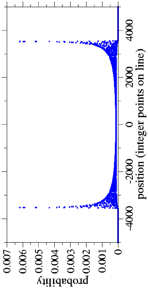
Figure 1: Probability distribution for a quantum walk on the line after 5000 steps, using a Hadamard coin, equation (2), and a symmetric initial state $(\mbox{$|R,0\rangle$}+i\mbox{$|L,0\rangle$})/\sqrt{2}$. Only even positions shown since odd positions are unoccupied.

The position probability distribution of a quantum walk on a line is by now well-known, an example with a Hadamard coin operator, and initial state of $\frac{1}{\sqrt{2}}(\mbox{$|R\rangle$}+i\mbox{$|L\rangle$})\otimes\mbox{$|0\rangle$}_{x}$ after 5000 time steps is shown in figure 1.

II.1 Entanglement between coin and position

Since the quantum walk dynamics are unitary, the system remains in a pure state and we can use the entropy of the reduced density matrix of the coin to quantify the entanglement between the coin and the particle’s position,

$$E_{c}(t)=-\sum_{j}\lambda_{j}\log_{2}(\lambda_{j})$$ (6)

where $\{\lambda_{j}\}$ are the eigenvalues of the reduced density matrix of the coin at time $t$ (in the case of the walk on a line there are just two eigenvalues).

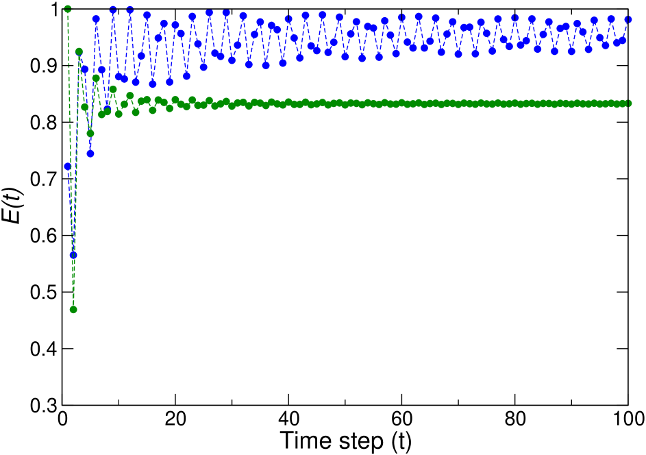
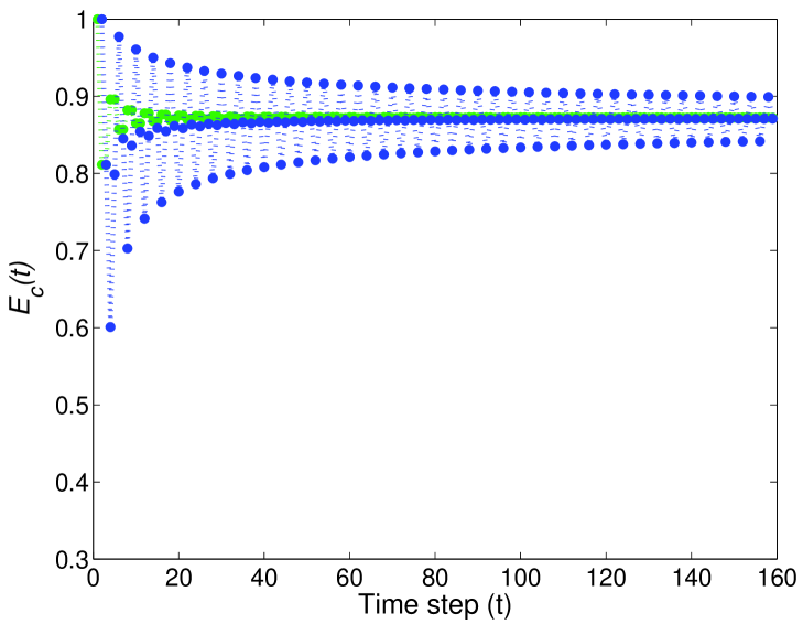
Figure 2: (Left) Entanglement $E_{c}(t)$ for a walk on a line with a biased coin, equation (4) with $\rho=0.2$, and two different initial states, asymmetric $|R,0\rangle$ (blue) and symmetric $(\mbox{$|R,0\rangle$}+i\mbox{$|L,0\rangle$})/\sqrt{2}$ (green) Annabestani (2008). (Right) Entanglement $E_{c}(t)$ for a walk on a line with coin operator bias $\rho=0.5$ (a Hadamard coin), and the same two initial states.

Figure 2 shows how $E_{c}(t)$ varies for different initial coin states using a coin operator equation (4), with bias $\rho=0.2$. This shows that the entanglement approaches a limiting value that varies between zero and one depending on the initial state of the coin. The rate of convergence to the limiting value also depends on the initial state of the coin, with symmetric initial states ($\eta=0.5$) converging fastest (i.e. oscillations about the asymptotic value die away fastest).

II.2 Limiting value of the entanglement

For the unbiased (Hadamard) coin operator ($\rho=0.5$), whatever initial coin state $|\psi_{0}\rangle$ is chosen, the asymptotic value of the entanglement $E_{c}(t\rightarrow\infty)\longrightarrow E_{\text{Had}}\simeq 0.872$. Note added: this statement is not correct, the asymptotic value varies with the initial coin state Gattner (2006); Abal et al. (2006). However, the rate of convergence is very different for different initial coin states, with more symmetric initial states converging faster, see figure 2.

For biased coin operators, the picture is more complicated. We have studied the limiting value of the entanglement for two different initial state, $|L,0\rangle$ (asymmetric) and $(\mbox{$|L,0\rangle$}+i\mbox{$|R,0\rangle$})/\sqrt{2}$ (symmetric), see figure 3.

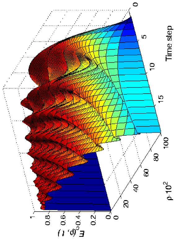
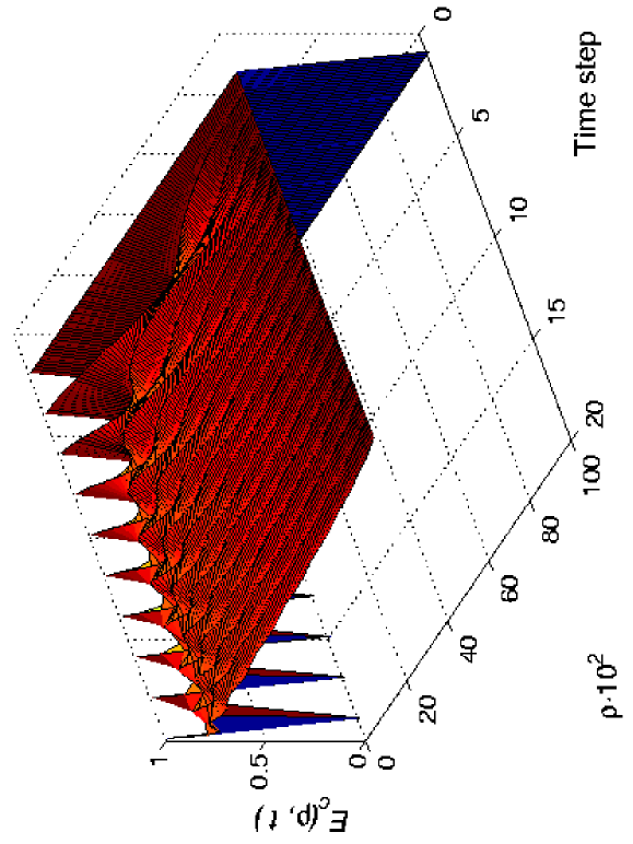
Figure 3: Entanglement $E_{c}(t)$ for a walk on a line: asymmetric initial coin state $|L\rangle$ shown left, and symmetric initial coin state, $(\mbox{$|L\rangle$}+i\mbox{$|R\rangle$})/\sqrt{2}$ shown right, for varying coin bias $\rho$, over 20 time steps.

In the asymmetric case the entanglement converges to a limiting value for all $\rho$. The limiting value of the entanglement $E_{\infty}(\rho)$ increases monotonically from $0$ ($\rho=1$) to $1^{-}$ ($\rho=0^{-}$) and is discontinuous at $\rho=0$. For $\rho=0$ the coin operator becomes the Pauli spin operator $\sigma_{x}$ and the entanglement is zero for all time steps, showing the coin and particle remain disentangled. In the symmetric case the entanglement converges to a limiting value for all except the extreme case of $\rho=0$ where the entanglement oscillates between the minimum and maximum values $0$ and $1$, as can easily be verified analytically. The asymptotic value of the entanglement $E_{\infty}(\rho)$ increases to $1$ as $\rho$ increases. The other variable factor is the period of the oscillations about the convergent value. In both cases, except for $\rho=0$ this period increases to infinity as $\rho\rightarrow 1$. As noted for the unbiased (Hadamard) coin, the rate of convergence to the asymptotic entanglement is faster for the symmetric initial coin state.

II.3 Rate of convergence

In order to quantify the rate of convergence of the entanglement to its limiting value, we considered the magnitude of the entanglement at a fixed time while varying the initial state. It is convenient to write the initial coin state as

$$\mbox{$|\psi_{0}\rangle$}=\cos(\alpha)\mbox{$|R\rangle$}+\sin(\alpha)e^{i\beta}\mbox{$|L\rangle$},$$ (7)

where $\eta=\cos^{2}(\alpha)$. Figure 4 shows how the amplitude varies with both $\alpha$ and $\beta$. First consider the case where $\alpha=\frac{\pi}{4}$ for $\eta=0.5$ i. e. a symmetric initial state. We find that the entanglement is proportional to $\cos^{2}(\beta)$ along the dotted line in figure 4. We can also fit a formula for the minimum,

$$\alpha=\frac{\pi}{8}\cos(\beta)+\frac{\pi}{4}.$$ (8)

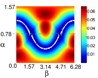
Figure 4: Amplitude of oscillations of entanglement versus initial coin state parameters $\alpha$ and $\beta$, for a Hadamard coin operator applied for 200 time steps.

This is the white line in the blue region in figure 4 where the entanglement oscillations are smallest, i.e., fastest convergence.

To summarise the results for the quantum walk on a line, we find the various behaviours of the entanglement are governed as follows. The asymptotic value $E_{\infty}$ reached by the entanglement is a function of both the coin bias $\rho$ and the initial state $|\psi_{0}\rangle$. For a fixed number of time steps $t$, the period of oscillation of the entanglement $E_{c}(t)$ around $E_{\infty}$ is a function of $\rho$ only. For the special case of $\rho=0.5$, an unbiased coin, $E_{\infty}=E_{Had}$ has the same value of $0.872\dots$ for all choices of initial coin state $|\psi_{0}\rangle$.

III Lattices in two spatial dimensions

III.1 Higher dimensional coins

For lattices with more than two edges meeting at each vertex, there is a far wider range of unitary coin operators, since the coin must now have as many degrees of freedom as there are choices of path. Since the range of higher dimensional coin operators is too large for systematic numerical study, for the remainder of this paper we concentrate on two natural choices. The Grover operator was first introduced by Moore and Russell Moore and Russell (2002) in their study of quantum walks on the hypercube. Based on Grover’s diffusion operator, it has elements $[C^{(\text{G})}_{d}]_{i,j}=\frac{2}{d}-\delta_{ij}$, i.e.,

$$\mathbf{C}_{d}^{(G)}=\left(\begin{array}[]{ccccc}2/d-1&2/d&\ldots&2/d\\ 2/d&2/d-1&\ldots&2/d\\ \vdots&\vdots&&\vdots\\ 2/d&2/d&\ldots&2/d-1\\ \end{array}\right).$$ (9)

For example, the $d=3$ case is

$$\mathbf{C}_{3}^{(G)}=\frac{1}{3}\left(\begin{array}[]{rrr}-1&2&2\\ 2&-1&2\\ 2&2&-1\\ \end{array}\right).$$ (10)

Except in the $d=4$ case, the Grover coin is biased, since the incoming direction (corresponding to the diagonal entry) is treated differently from the outgoing directions. However, it is symmetric under interchange of any outgoing coin directions, and is in fact the symmetric unitary operator furthest from the identity. The $d=4$ Grover coin is the only unbiased Grover coin since all the entries are $\pm\frac{1}{2}$

$$\mathbf{C}_{4}^{(G)}=\frac{1}{2}\left(\begin{array}[]{rrrr}-1&1&1&1\\ 1&-1&1&1\\ 1&1&-1&1\\ 1&1&1&-1\\ \end{array}\right).$$ (11)

The DFT (discrete Fourier transform) coin is unbiased for all $d$, but asymmetric in that you cannot interchange the labels on the directions without changing the coin operator: each direction acquires its own phase shift. For $d=3$, it looks like

$$\mathbf{C}_{3}^{(D)}=\frac{1}{\sqrt{3}}\left(\begin{array}[]{ccc}1&1&1\\ 1&\omega_{3}&\omega^{2}_{3}\\ 1&\omega^{2}_{3}&\omega_{3}\\ \end{array}\right),$$ (12)

where $\omega_{3}=e^{2i\pi/3}$ and $\omega^{2}_{3}=e^{-2i\pi/3}$ are the complex cube roots of unity. The $d$-dimensional DFT coin can be written

$$\mathbf{C}_{d}^{(D)}=\frac{1}{\sqrt{d}}\left(\begin{array}[]{ccccc}1&1&1&\ldots&1\\ 1&\omega&\omega^{2}&\ldots&\omega^{d-1}\\ 1&\omega^{2}&\omega^{4}&\ldots&\omega^{2(d-1)}\\ \vdots&\vdots&\vdots&&\vdots\\ 1&\omega^{d-1}&\omega^{2(d-1)}&\ldots&\omega^{(d-1)^{2}}\\ \end{array}\right),$$ (13)

where $\omega$ is the complex $d$’th root of unity.

III.2 Cartesian lattice

For a 2-dimensional Cartesian grid, there are four edges meeting at each lattice site, so a $d=4$ dimensional coin is required. The quantum walk is a generalisation of the walk on a line. We tested both Grover and DFT coins ($d=4$ versions) and found a similar range of behaviours for the entanglement between the coin and the position as for the walk on a line, only compounded by having twice as many directions. So, for example, the period of the oscillations about the asymptotic value is now a more complicated pattern of two frequencies.

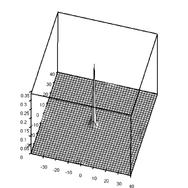
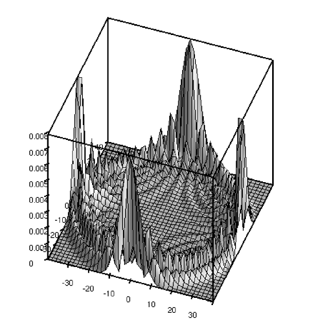
Figure 5: Typical (left) and ring-like (right) spreading distribution for a Grover coin on a 2-dimensional Cartesian lattice (from Tregenna et al. (2003)). Axes represent position ($x$ and $y$) with the $z$ axes indicating the probability of finding the particle at that position.

We looked for a correlation between the rate of convergence of the entanglement and the degree to which the quantum walk spreads out over the lattice. Most choices of initial state for the Grover and DFT coin operators produce a high probability of finding the particle on or near the starting point, with only one special initial state giving a high rate of spreading, compare the two distributions in figure 5, taken from Tregenna et al. (2003). Spreading is a property of random walks that can be useful for efficient, uniform sampling, compare Kendon and Tregenna (2003). The entanglement converges much faster for the quantum walk that spreads out in the ring, see figure 6. The entanglement between the coin and the position thus provides a way to monitor the progress and character of the walk.

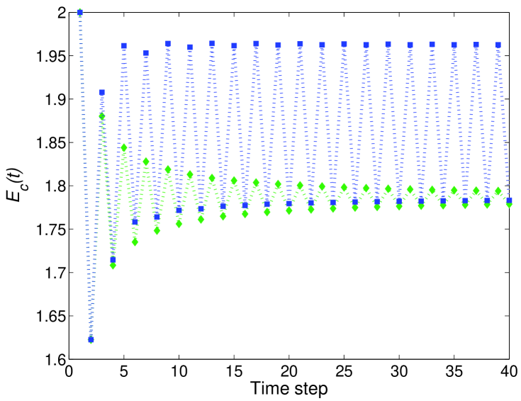
Figure 6: Entanglement $E_{c}(t)$ for the spike (blue) and ring (green) distributions on a 2D Cartesian lattice, using a Grover coin. A DFT coin operator produces a very similar result.

III.3 Triangular lattices

Higher dimensional lattices that lie in a plane (two spatial dimensions) can be constructed in a number of ways. We studied two examples: a tessellation of equilateral triangles produces a lattice with $d=6$; and adding diagonals to a Cartesian grid, makes a “first and second nearest neighbours” lattice with $d=8$. These are illustrated in figure 7.

Figure 7: Triangular lattices with (a) $d=6$ and (b) $d=8$.

We tested a number of different initial states with both Grover and DFT coins, again looking at correlations between the amount that a walk starting from the centre of the grid spreads and the oscillations in the entanglement. To quantify the spread we studied the mean square deviation of the probability distribution from the uniform probability distribution

$$\overline{\Delta P}^{2}(t)=\sum_{r}\left(|\psi(r,t)|^{2}-\frac{1}{N(t)}\right)^{2},$$ (14)

where $r$ is a lattice site in the set it is possible to reach after $t$ steps, and $N(t)$ is the number of such lattice sites (so $1/N(t)$ is the average probability per site). If the walk is spread out evenly over the lattice then $\overline{\Delta P}^{2}(t)$ will be small, whereas if it is concentrated on parts of the lattice, $\overline{\Delta P}^{2}(t)$ will be larger.

For the both the $d=6$ and $d=8$ grids, as on the rectangular grid, the Grover coin can produce two kinds of behaviour: fast spreading distributions and distributions concentrated nearly all close to the origin, depending on the choice of initial states. The amplitudes of the oscillations in the entanglement decrease quickly for fast spreading but only slowly for the distributions stuck near the starting point. This is illustrates in figures 8-9.

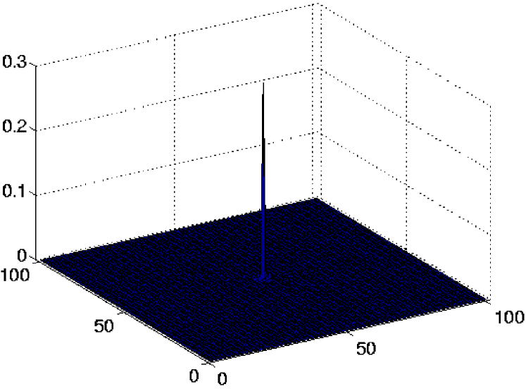
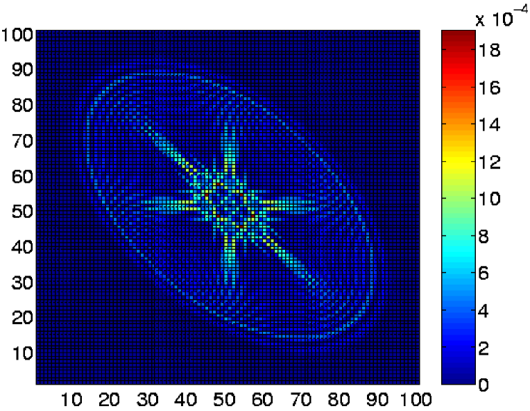
Figure 8: Probability distribution after 49 steps of a quantum walk on a $d=6$ grid using a Grover coin operator: (Left) starting with coin state $\frac{1}{\sqrt{d}}\sum_{i=1}^{d}|i\rangle$, at the point (50,50), and (Right) starting with coin state $\frac{1}{\sqrt{d}}\sum_{i=1}^{d/2}|i\rangle-\frac{1}{\sqrt{d}}\sum_{i=d/2+1}^{d}|i\rangle$. Axes represent position in the $xy$-plane and probability as in figure 5.

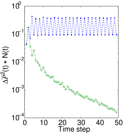
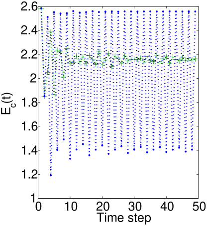
Figure 9: Spreading as indicated by the mean square deviation from the uniform distribution $\overline{\Delta P}^{2}(t)$ (left) and entanglement $E_{c}(t)$ (right) for the cases shown in figure 8 spike (blue) and ring (green).

In contrast to the Grover coin operator, the DFT coin produces good spreading for almost all chosen initial states and the entanglement converges faster for these cases. To investigate the correlation between the entanglement and the spreading of the walk more thoroughly, we wrote the initial coin state as

$$|\psi_{0}\rangle=\sum_{j=1}^{d}e^{i\phi_{j}}|j\rangle.$$ (15)

For $d=6$, we fixed one of the phases and varied the other $d-1$ over all the permutations, allowing repetitions of $\phi_{j}=\pi j/d$, ($j=1,\ldots,d$, total of $6^{6}$ values, thus) to see the interference effects on the spread. For the Grover coin operator, most of these states give a large $\overline{\Delta P}^{2}(t)$ while for the DFT most give a small $\overline{\Delta P}^{2}(t)$: the average (over these initial states) after $t=15$ steps is $\langle\overline{\Delta P}^{2}(t)\rangle=0.0501$ for the Grover and $\langle\overline{\Delta P}^{2}(t)\rangle=0.0015$ for the DFT walk. For the minimum $\overline{\Delta P}^{2}(t)$ in this set, the entanglement oscillations decay fastest, as seen in figures 9 (for $d=6$) and 11 (for $d=8$). The minimum values of $\overline{\Delta P}^{2}(t)$ occur for the initial states $\{\phi_{j}\}=(0,0,0,0,0,0)$ for the Grover coin operator and $\{\phi_{j}\}=(0,0,4,1,1,5)$ for the DFT coin operator.

For $d=8$, we fixed one of the phases and varied the other $d-1$ over only the following subsets of all the arrays of $\phi_{j}=\pi j/d$: (i) $j\in{0,d-1}$, $\{\phi_{j}\}=(0,0,0,0,0,0,0,0),(0,0,0,0,0,0,0,d-1),\ldots,(d-1,d-1,\ldots,d-1,d-1,0)$; (ii) permutations of $(0,1,2,\ldots,d-1)$ (without repetitions) to see the interference effects on the spread. Although we didn’t vary over as large a range as in the $d=6$ case, we could observe a similar behaviour: better spread for DFT against Grover, entropy converging quickly for better spread.

The average (over these initial states) after $t=15$ steps is $\langle\overline{\Delta P}^{2}(t)\rangle=0.0508$ for the Grover and $\langle\overline{\Delta P}^{2}(t)\rangle=0.0027$ for the DFT walk. (For the $d=8$ grid $N(t)=(2t+1)^{2}$, since there are diagonals everywhere). The minimum values of $N(t)\overline{\Delta P}^{2}(t)$ occur for the initial states $\{\phi_{j}\}=(0,0,0,0,0,0,0,0)$ for the Grover coin operator and $\{\phi_{j}\}=(0,7,7,7,7,0,0,7)$ for the DFT coin operator.

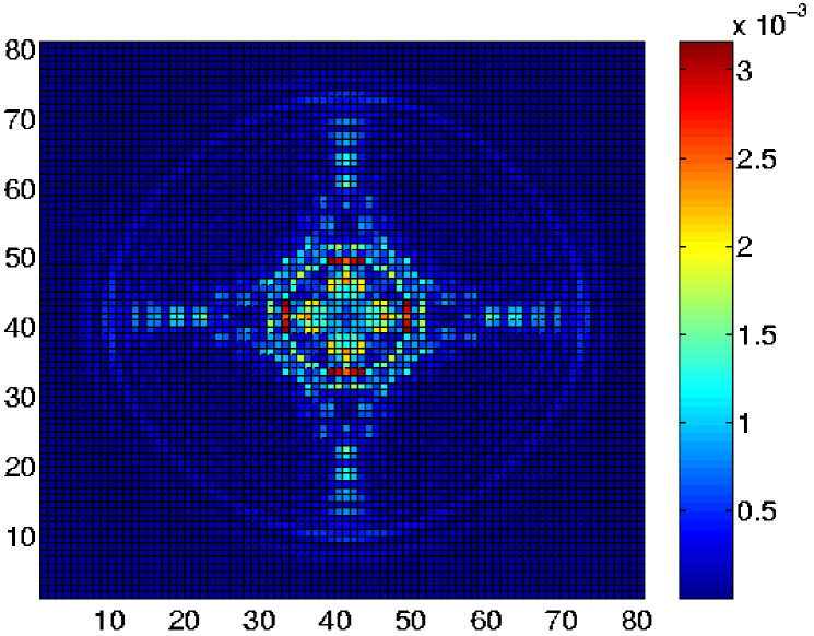
Figure 10: Grover coin on $d=8$ grid, after 39 time steps, start with coin state $\frac{1}{\sqrt{d}}\sum_{i=1}^{d/2}|i\rangle-\frac{1}{\sqrt{d}}\sum_{i=d/2+1}^{d}|i\rangle$. Axes represent position in the $xy$-plane and probability as in figure 5.

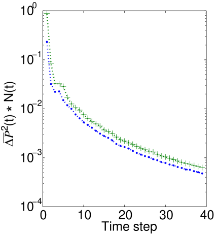
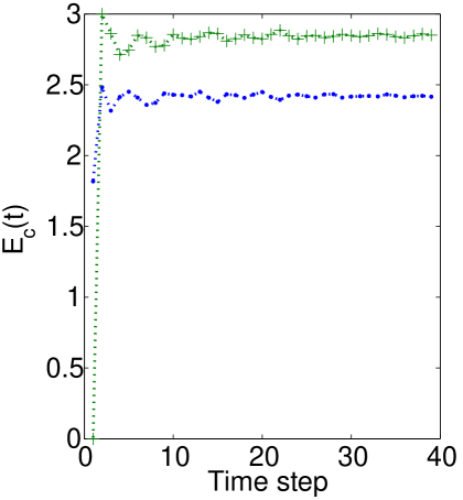
Figure 11: Spreading as indicating by the mean square deviation from the uniform distribution $\overline{\Delta P}^{2}(t)$ (left) and entanglement $E_{c}(t)$ (right) for the DFT coin operator on $d=8$ grid, after 39 time steps, starting with coin states $\frac{1}{\sqrt{d}}\sum_{i=1}^{d}|i\rangle$ (blue) and $\frac{1}{\sqrt{d}}\sum_{i=1}^{d/2}|i\rangle+i\frac{1}{\sqrt{d}}\sum_{i=d/2+1}^{d}|i\rangle$ (green).

For the $d=8$ grid we also tested Hadamard coins (a simple 2D Hadamard coin for each of the 4 pairs of opposite directions) and found they displayed similar properties to the DFT coin.

Thus, for all tested coin operators and coin initial states, we have verified that those walks with good spreading also show small amplitudes of oscillation in the entanglement of the coin, pointing to a quick convergence. In particular, the DFT and Hadamard coin operators produce faster spreading than the Grover coin for most choices of initial state on these lattices of higher degree. This can be explained by noticing that for $d>4$, the Grover coin is biased so that it favours returning along the edge that it arrived from. This will tend to reduce its spreading power. The DFT coin is unbiased, so its spreading power is affected only by how the different phases cause interference effects. For larger $d$, there are more different phases, so less opportunities for them to all cancel out. The Hadamard coin is also unbiased, and it does not mix between the different orientations of the pairs of edges, so on these triangular lattices it produces a spreading equivalent to the spreading on a line.

IV Walks on finite regular graphs

We now turn to quantum walks on graphs with a fixed number of vertices so the walk is bounded and the notion of spreading is no longer the relevant property. Quantum walks on finite graphs were first investigated by Aharonov et al Aharonov, D et al. (2001), who showed that while the instantaneous distribution of a quantum walk on these graphs does not converge (being unitary and reversible), a suitably defined time-averaged distribution always converges, though this distribution need not be uniform (in the classical case the limiting distribution is always uniform). The interesting questions are thus how fast the quantum walk converges to the limiting time-averaged distribution, and whether the distribution is uniform. We are also interested in whether the walk shows periodic behaviour in the instantaneous distribution Tregenna et al. (2003), and if so, under what conditions.

IV.1 $N$-cycles

The quantum walk on a line can be converted to an $N$-cycle by taking a line segment of length $N$, and applying periodic boundary conditions. Clearly, for $t$ greater than $N/2$, when the walk starts to wrap around on itself, the evolution will be more complicated than a line. Cycles with odd or even values of $N$ give different results. For an even cycle, only even (odd) positions are occupied after an even (odd) number of time steps, but for an odd cycle, after the first $(N+1)/2$ steps, both even and odd positions are occupied at the same time. We use the same coin operator as for the walk on the line, given by equation (1). We observed that the entanglement of the coin, apart from the particular cases identified by Tregenna et al Tregenna et al. (2003) in which the walk is periodic, shows no regular pattern, being apparently chaotic. We give two examples illustrating this in figure 12.

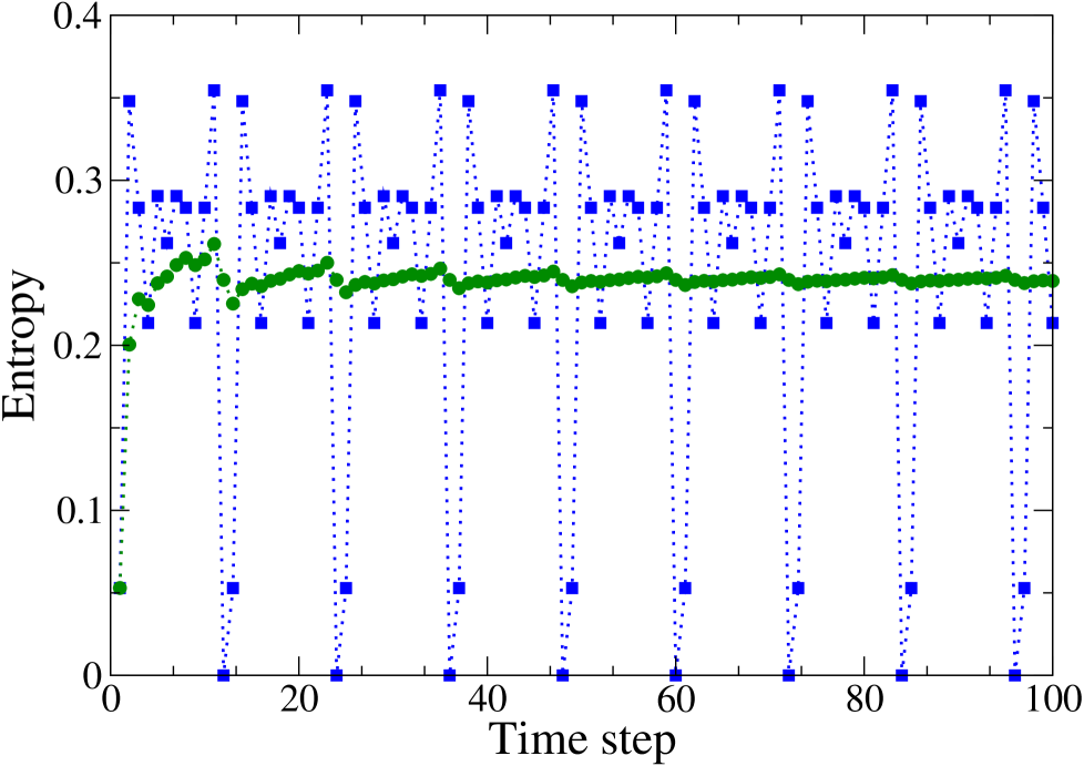
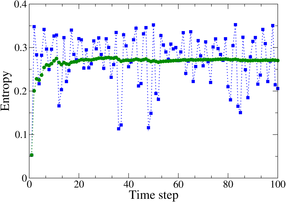
Figure 12: (Left) Entropy versus time step for eight-cycle with symmetric initial coin state. (Right) Entropy versus time step for 16-cycle with symmetric initial coin state. Both instantaneous (blue) and time averaged (green) values of the entropy are shown.

Since the entanglement follows the instantaneous state of the system, it does not tell anything useful about the mixing properties of the time-averaged distribution. We also calculated the time-averaged entanglement (shown in figure 12) and this appears to converge to a steady value at roughly the same rate as the distribution converges to its limiting distribution. This is shown for a seven-cycle in figure 13.

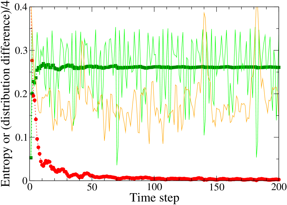
Figure 13: Comparison of time-averaged entropy (thick green) with convergence to time-averaged limiting (uniform in this case) distribution (thick red) for a seven-cycle with symmetric initial coin state and Hadamard coin operator. The difference between the time-averaged distribution and the limiting distribution is scaled by a factor of 0.25 to make the range of fluctuations roughly comparable with the entropy, as shown by the instantaneous entropy and distribution difference (thin lines).

IV.2 Cycles with diagonals

Next we consider the case where there are three or more possible directions that the particle can take. As a generalisation of the cycles, we take the case (for $N$ even) where opposite vertices of the $N$-cycle are joined to give three possible directions for the particle. Figure 14 explains how this works.

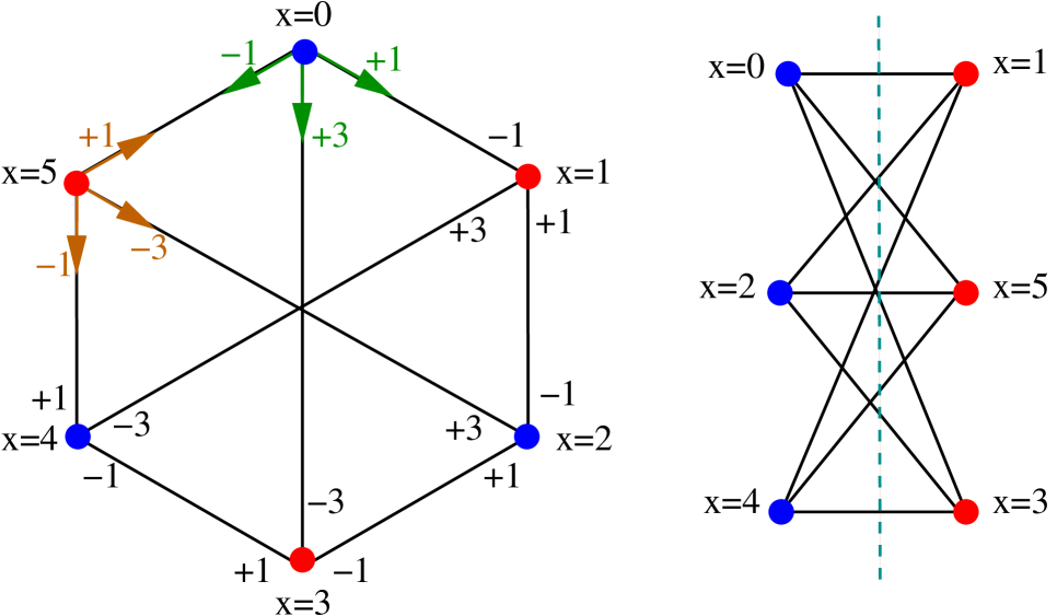
Figure 14: A six-cycle where the numbers $\pm 1$, and $\pm 3$ label the directions which the particle can take. This is an example of a complete bipartite graph, as redrawn in equivalent form on the right. Each blue vertex is connected to every one of the red vertices and vice versa; all the edges cross between the two sets of vertices (divided by the dashed line).

The third possible path of the particle connects the original position ($x=0$) to the opposite position ($x=3$) of the cycle, and likewise for the other two opposite pairs. The edges of the cycle need to be consistently labeled (see Kendon and Sanders (2004); Ambainis (2003)), and here we have chosen to label each end of the edges with either $-1$, 1, $-3$ or 3, such that adding the vertex and edge label gives the vertex label at the other end of that edge. This means that as the particle traverses the edge, the sign of the coin state must flip, so we adjust the conditional shift operation to act as

$$S\mbox{$|c,v\rangle$}=\mbox{$|-c,v+c(\text{mod $N$})\rangle$},$$ (16)

where $v\in\{0\dots(N-1)\}$ is the vertex and $c$ is the coin state, compare equation (5). Although this means we are using more coin states than the degree of the graph (four instead of three), at any single vertex only three of the four coin states are actually used, and we pad the coin operator with zeros (one on the diagonal) for the unused coin state so it operates correctly (as a Grover or DFT coin) on the three-dimensional subspace. More details on how to do this for the general case of a graph with vertices of various degrees can be found in Kendon and Sanders (2004).

The evolution of the walk is determined by the coin operator: we used the $d=3$ Grover and DFT coins, equations (10) and (12) respectively. For $N=6$, the entanglement is periodic with period four, as shown in figure 15 (Left).

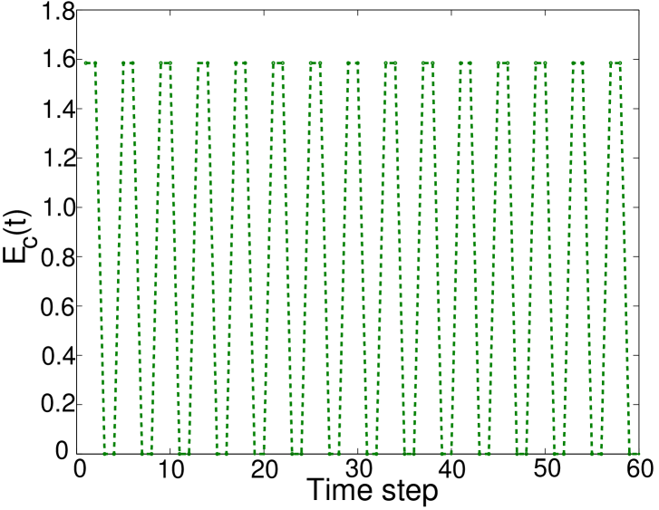
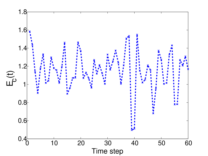
Figure 15: (Left) Entanglement $E_{c}(t)$ for the graph of figure 14 using a DFT coin operator and a symmetric initial coin state. (Right) Entanglement $E_{c}(t)$ for 10-cycle with diagonals and a DFT coin operator.

For all other values of $N$ that we tested, the $N$-cycles plus diagonals showed no regularity, and the entanglement followed a complicated pattern, as illustrated in figure 15 (Right) for the case of $N=10$.

IV.3 Complete bipartite graphs

The six-cycle with opposite vertices linked is an example of a complete bipartite graph. In a bipartite graph the vertices can be divided into two distinct sets such that every edge connects between the two sets. A bipartite graph is complete if, in addition, each vertex in one set is connected to every vertex in the other set. These conditions fix the relationship between the number of vertices and the degree of the graph: a complete bipartite graph of degree $d$ has $N=2d$ vertices, we denote it by $K_{d,d}$. These graphs can be obtained from the $N$-cycle by adding edges between every pair of vertices $(i,j)$ in which $i$ is odd and $j$ is even. We can label the directions from each vertex as $\pm 1,\pm 3,\ldots,\pm(d-1)$, as shown in figure 14 for $d=3$, i.e., $N=6$. Ahmadi et al. Ahmadi et al. (2003) studied the continuous time quantum walk on similar graphs, looking for instantaneous mixing (i.e., a uniform distribution obtained at a particular instant in the time evolution of the quantum walk). They found only a small number of examples of instantaneous mixing, for regular complete and cyclic graphs with no more than four vertices. This is in sharp contrast to classical random walks, which approach a uniform distribution as they evolve on all well-behaved graphs. Periodic behaviour is also a property of the instantaneous distributions, though a slightly less stringent requirement than instantaneous mixing.

We can show analytically that the Grover walk on $K_{d,d}$ is periodic with period 4, by looking at the evolution operator $U=S\cdot(\leavevmode\hbox{\small 1\kern-3.2pt\normalsize 1}\otimes C_{d}^{(G)})$ in Fourier space. With our chosen edge labeling the shift operator acts as in equation (16). Taking a FT on the vertex space only,

$$|v\rangle=\frac{1}{\sqrt{N}}\sum_{k=1}^{N}e^{2\pi ikv/N}|k\rangle,$$ (17)

shows that the shift acts as

$$S|v,c\rangle=\frac{1}{\sqrt{N}}\sum_{k=1}^{N}e^{2\pi i(v+c)k/N}|k,-c\rangle$$ (18)

and then

$$S_{k}|k,c\rangle=e^{2\pi ick/N}|k,-c\rangle,$$ (19)

meaning that $S$ is block-diagonal in the FT basis. Represent it by

$$S_{k}=\left(\begin{array}[]{cccccc}0&\omega^{k}&0&0&\ldots&0\\ \omega^{-k}&0&0&0&\ldots&0\\ 0&0&0&\omega^{+3k}&\ldots&0\\ 0&0&\omega^{-3k}&0&\ldots&0\\ \vdots&\vdots&\vdots&\vdots&\ddots&\vdots\\ 0&0&0&0&\ldots&\omega^{-k(d-1)}\\ \end{array}\right),$$ (20)

in which $\omega=e^{2\pi i/N}$, and the last entry is in the diagonal for the case where $d$ is odd, otherwise the last block is similar to the others. In this basis, the ($Nd$-dimensional) evolution operator $U=S\cdot(\leavevmode\hbox{\small 1\kern-3.2pt\normalsize 1}\otimes C_{d}^{(G)})$ factorises into a set of $N$ matrices $U_{k}$ each of dimension $d$, with $U_{k}=S_{k}\cdot C_{d}^{(G)}$. From this one can check explicitly that $U_{k}^{4}=\leavevmode\hbox{\small 1\kern-3.2pt\normalsize 1}$, which means that the walk has a period of $4$. Alternatively, by looking at the eigenvalues of $U_{k}$ we can also verify the periodicity. $U_{k}$ has eigenvalues $\pm 1$ and $e^{i\theta_{k}}$, with $\cos\theta_{k}=\frac{-1}{d}\sum_{c=1,3,\ldots,(d-1)}\cos\frac{2\pi c}{N}$ (method used in Ambainis (2004)), which reduce to $\pm i$ when $d=N/2$.

Using numerical simulations with a DFT coin on complete bipartite graphs we found no examples of periodicity.

V Walks on the “Glued trees” graph

We now turn out attention to the special graph used by Childs et al. Childs et al. (2003) for their algorithm with an exponential speed up. An example of this “glued trees” graph with tree depth $N=4$ is shown in figure 16 (right). At the centre, each leaf node has two edges joining it to the leaf nodes of the other tree so, except for the entrance and exit, exactly three edges meet at each node.

Figure 16: Left: regularly glued binary tree graph. Right:“glued trees” graph used in the algorithm of Childs et al. (2003). Example shown is for $N=4$, with $2N+2=10$ columns and $2(2^{(N+1)}-1)=62$ nodes. The gap between columns 4 and 5 is for clarity in the figure and is not significant in the algorithm.

The problem is to travel via the edges from node to node as quickly as possible starting at the entrance and finishing at the exit. The time taken to reach the exit is an example of a “hitting time” (see Kempe Kempe (2003b) for definitions and an earlier example of a “hitting time” quantum walk problem). A similar graph with a regular join at the leaves is also shown in figure 16 (left). This graph is easy to traverse with a classical algorithm because it is easy to identify the middle (in this case because the middle nodes have only two edges joining them, but a regular pattern of two edges per node is also classically tractable). The randomly glued edges joining the two halves of the graph in figure 16 (right) disguise the join, and a classical algorithm will get lost at this point, taking on average exponentially longer to emerge at the exit.

Childs et al. use a continuous time quantum walk Farhi and Gutmann (1998) for their algorithm. The adjacency matrix $\mathbf{A}$ of a graph is an $N\times N$ matrix with entries $A_{ij}=1$ iff there is an edge joining nodes $i$ and $j$, all other entries in $\mathbf{A}$ are zero. For an undirected graph (edges can be traversed in either direction, from $i\rightarrow j$ and $j\rightarrow i$), $\mathbf{A}$ is symmetric. Thus it can be used to form the Hamiltonian for the quantum walk:

$$i\frac{d}{dt}\mbox{$\langle x|\psi(t)\rangle$}=\sum_{y}^{N}\mbox{$\langle x|$}\mathbf{H}\mbox{$|y\rangle$}\mbox{$\langle y|\psi(t)\rangle$},$$ (21)

with $\mathbf{H}=\gamma\mathbf{A}$ where $\gamma$ is the transition probability, and where $x,y$ are nodes in the graph. The solution may be written

$$\mbox{$|\psi(t)\rangle$}=e^{-i\gamma\mathbf{A}t}\mbox{$|\psi(0)\rangle$},$$ (22)

though of course actually calculating it for specific instances of $\mathbf{A}$ and $|\psi(0)\rangle$ is in general a nontrivial task. The proof Childs et al. (2003) that the quantum walk is exponentially faster than any classical algorithm involves detailed consideration of oracles, colourings and simulation of a continuous time quantum walk on a discrete gate-model quantum computer. We will not need to discuss these details here. Figure 17 shows an example of the propagation of the continuous time walk through the glued trees graph in terms of the column positions shown in figure 16.

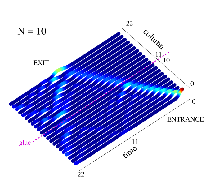
Figure 17: Propagation of the continuous time quantum walk on a glued trees graph for tree depth $N=10$, run for 44 time steps.

A discrete time walk can also traverse this graph efficiently if a three dimensional Grover coin is used Watrous (2002); Tregenna et al. (2003). An example of the propagation using a Grover coin operator is shown in figure 18.

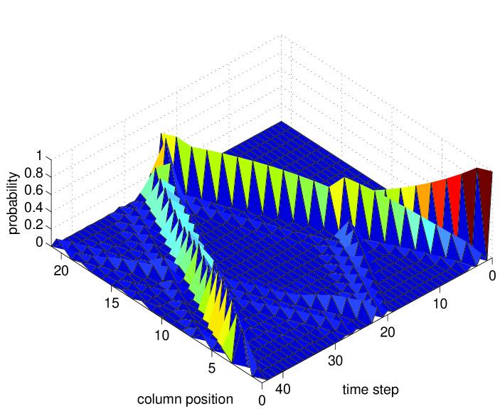
Figure 18: Propagation of the discrete quantum walk using the Grover coin operator on a glued trees graph for tree depth $N=10$, run for 44 time steps.

As noted by Tregenna et al. Tregenna et al. (2003), the fast hitting time obtained with a quantum walk is highly sensitive to the symmetry of the problem: for quantum walks starting at a node other than the entrance, the exit becomes exponentially harder to find and the quantum walk does no better than a classical algorithm.

Tregenna et al. also noted that that if a DFT coin operator is used instead of a Grover coin operator on the “glued trees” graph, the quantum walk stays near the starting point and does not spread out even as far as a classical random walk. We consider how this picture changes if we increase the branching rate of the trees that form the graph. In other words, we make a similar graph using a pair of trinary trees (branching rate 3) and quaternary trees (branching rate 4) and so on for arbitrary branching rate $B$. This is illustrated in figure 19.

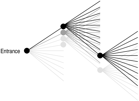
Figure 19: Detail of a graph with higher branching rate at each node. The branching rate in this example is $B=10$, and the degree of each node (except the entrance and exit nodes) includes the edge from the parent node so is $d=B+1=11$.

V.1 Mapping to a walk on the line

Despite the random connections in the centre, the “glued trees” graph with any branching rate is still highly symmetric. Provided the initial state used at the entrance node respects the symmetry, the whole quantum walk process can be mapped to a walk on a line corresponding to the column positions shown in figure 16, with different biases in the probabilities for moving right or left at each step. The mapping for the continuous time walk is given in Childs et al. (2003) for branching rate $B=2$. For arbitrary branching rate this generalises to give a Hamiltonian for column positions $j$ with non-zero matrix elements

$$\mbox{$\langle j|$}H\mbox{$|j+1\rangle$}=\left\{\begin{array}[]{ll}\sqrt{B}\gamma&0\leq j<N,\,N<j\leq 2N\\ B\gamma&j=N\\ \end{array}\right.$$ (23)

and $\mbox{$\langle j+1|$}H\mbox{$|j\rangle$}=\mbox{$\langle j|$}H\mbox{$|j+1\rangle$}$. We have a choice for the hopping rate $\gamma$. In order to make a fair comparison between different branching rates $B$, we take $\gamma=B^{-1/2}$. This makes the non-zero matrix elements of $H$ unity, except at the glue, corresponding to unit hopping rate between column positions in the mapped-to-line version of the quantum walk, for all choices of $N$ and $B$.

For the discrete time quantum walk the mapping is coin specific, and only works when the coin operator preserves the symmetry of the graph so the amplitude of the quantum walk is the same on all nodes of each column. To perform the mapping for the Grover coin operator given by equation (9), we consider one step of the evolution at a typical node in the left hand tree. Our notation is shown in figure 20.

Figure 20: Typical node in left hand tree before and after the coin operator is applied, showing our notation for mapping the walk to a line, $P$, $Q$, $\{C_{i}\}$, $\{D_{i}\}$ $R_{I}$, $R_{O}$, $L_{I}$, $L_{O}$ are amplitudes.

We assume that $C_{1}=C_{2}\dots=C_{B}=C$ and $D_{1}=D_{2}\dots=D_{B}=D$. Applying the Grover coin operator gives two relationships between the incoming and the outgoing amplitudes,

$$D = \frac{2}{B+1}P+\frac{B-1}{B+1}C$$

$$Q = \frac{1-B}{B+1}P+\frac{2B}{B+1}C.$$ (24)

We then require $B^{j}P^{2}=R^{2}_{I}$ and $B^{j}\sum_{\alpha}C^{2}_{\alpha}=L^{2}_{I}$ for the incoming probabilities on the full tree and on the line, similarly $B^{j}Q^{2}=L^{2}_{O}$ and $\sum_{\alpha}D^{2}_{\alpha}=R^{2}_{O}$ for the outgoing probabilities. This gives the relationship between the amplitudes on the full tree and on the line (independent of choice of coin operator),

$$P=B^{-j/2}R_{I} C=B^{-(j+1)/2}L_{I}$$

$$Q=B^{-j/2}R_{O} D=B^{-(j+1)/2}L_{O}$$ (25)

Substituting into equation (24) gives the $2\times 2$ operator for a quantum walk on a line corresponding to the Grover coin operator,

$$R_{O} = \frac{2\sqrt{B}}{B+1}R_{I}+\frac{B-1}{B+1}L_{I}$$

$$L_{O} = \frac{1-B}{B+1}R_{I}+\frac{2\sqrt{B}}{B+1}L_{I}.$$ (26)

The right hand tree is a mirror image of the left hand tree, so for that we just exchange $L$ and $R$ in the above equations. Unlike the continuous time walk, there is nothing special for the random edges in the glue, the amplitude for traversing each edge is determined by the coin operator at the nodes, and this coin operator is different for each half of the tree.

For the entrance and exit nodes we need to consider the most general choice in $d$ dimensions that respects the symmetry of the graph. As explained in Kendon and Sanders (2004), although the roots of the tree are only of degree $d-1=B$, we can pad the extra coin dimension with a piece of the identity operator so we have $d$ dimensional coins throughout the walk. This has the added effect of allowing an extra arbitrary phase, the most general form of the coin operator at the entrance and exit nodes takes the form

$$C_{\text{{end}}}=\left(\begin{array}[]{cc}e^{i\phi}C^{(B)}&\mathbf{0}\\ \mathbf{0}&1\\ \end{array}\right),$$ (27)

where $C^{(B)}$ is a suitably symmetric coin operator of dimension $B=d-1$, with an extra arbitrary phase $\phi$, and the boldface zeros fill in the row and column to make $C_{\text{{end}}}$ have dimension $d$. We then map $C_{\text{{end}}}$ to a walk on the line, which gives a reflection with a phase shift (that may be chosen independently at the entrance and the exit),

$$R_{O} = e^{i\phi_{1}}L_{I}\text{\hbox{}\hskip 10.00002pt {Entrance}}$$

$$L_{O} = e^{i\phi_{2}}R_{I}\text{\hbox{}\hskip 10.00002pt {Exit}}.$$ (28)

This mapped-to-the-line operator already tells us how the Grover coin operator will behave in the limit of large branching rate. Equation (26) becomes $-i\sigma_{y}$ as $B\rightarrow\infty$, for which the walk on a line simply oscillates between the initial and neighbouring nodes, making no further progress along the line. Thus we expect the probability of reaching the exit to fall towards zero as $B\rightarrow\infty$.

We can relate the entanglement between the coin and the position on the line to the entanglement between the coin and the position in the walk on the full graph. To calculate the entanglement, we calculate the entropy of the reduced density matrix for the coin (by tracing over the position) and then obtain the eigenvalues of this density matrix, from which the entropy is calculated according to equation (6). For a two-dimensional matrix the eigenvalues are the solution of a quadratic equation, for a $d$-dimensional coin the eigenvalues are the solution of a polynomial of order $d$. By calculating the reduced density matrices for the full walk and the mapped-to-line versions, and comparing the polynomials we find, for example, for the Grover coin case, the polynomials are related by

$$f^{(B)}_{\textsc{full}}(x)=(-x)^{B-1}(x^{2}-(a_{B}+Bd_{B})x+B(a_{B}d_{B}-c^{2}_{B}))=(-x)^{B-1}f^{(B)}_{\textsc{line}}(x),$$ (29)

where $a_{B}$, $c_{B}$, $d_{B}$ are time dependent coefficients. The roots of this polynomial give the eigenvalues and thence the entropy of the reduced density matrix, which measures the entanglement. Thus we see that the entanglement is the same between the coin and position in the mapped-to-line walk as in the corresponding full walk. We studied the entanglement for the walk on the glued trees graph, but it did not provide useful indications of the progress of the walk, so we do not present any of these results here.

V.2 Variation with tree depth $N$

We first restrict our attention to the original problem with branching rate $B=2$, and consider what happens when the tree depth $N$ is varied. The quantum walker does not arrive the exit with certainty after a short number of time steps. However, the probability of finding it at the exit node shows a clear peak after roughly the number of steps it takes to walk deterministically from entrance to exit by the shortest route. If this peak is large enough (polynomial in $N$ and $B$), one can simply repeat the quantum walk a polynomial number of times to increase the success probability to near certainty (probability amplification).

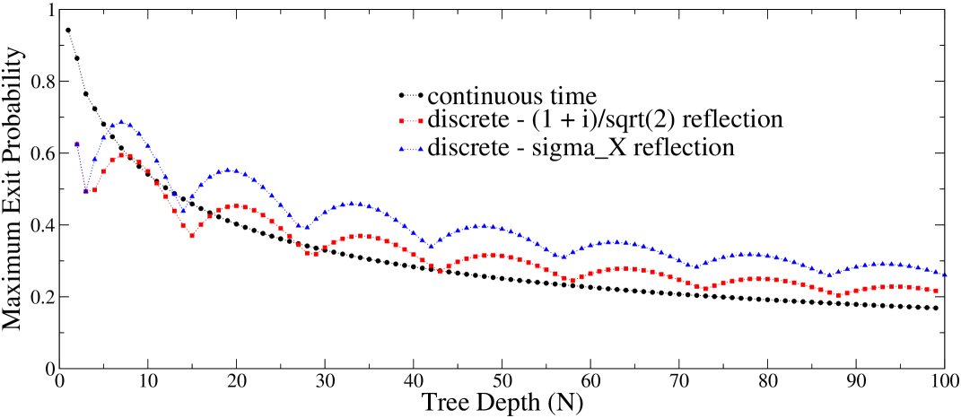
Figure 21: Variation of exit probability with tree depth on the “glued trees” graph with branching rate $B=2$ for the continuous time quantum walk (black) and the discrete quantum walk with a Grover coin using two different reflection phases as detailed in the key (red and blue).

We studied both continuous time and discrete time quantum walks using simulations with the dynamics mapped onto a walk on the line. For the continuous time walk the results are straightforward, given by the black line in figure 21. This is well-fit for large $N$ by $P(\text{{exit}})\sim N^{-2/3}$, as predicted by Childs et al. Childs et al. (2003), who derive the scaling of the Green’s function to be $\sim N^{-1/3}$ at the peak.

For the discrete time walk, as noted in the previous section, we have a choice about what to do at the entrance and exit where the nodes are of degree two rather than three. We tested two examples of choices of phase shifts, equation (27), using the same phase at both entrance and exit. The 2D version of the Grover coin operator is $\sigma_{x}$, which produces no phase shift when mapped to the line. Another possible symmetric 2D coin operator is

$$\mathbf{C}_{2}^{(\text{S})}=\frac{1}{\sqrt{2}}\left(\begin{array}[]{rr}1&i\\ i&1\\ \end{array}\right).$$ (30)

Mapped to the line, this produces a phase shift of $(1+i)/\sqrt{2}=e^{i\pi/4}$. The different phases give different results due to the different interference effects. Results for both are also shown in figure 21. They produce a slightly higher exit probability than the continuous time walk for most values of $N$, but follow the same scaling of $P(\text{{exit}})\sim N^{-2/3}$ (numerical data up to $N=10000$ not shown in figure 21 was used for the fitting). This corresponds with the analytic solution for a simple walk on a line found by Ambainis et al. Ambainis et al. (2001), which gives the scaling of the peak amplitude as $\sim N^{-1/3}$. The mapped-to-the line quantum walk is not exactly the same as the simple walk on an infinite line, but the scaling of the peak should be similar, up to the first reflection at the exit. This scaling, being polynomial in $N$, does not affect the exponential speed up of the algorithm. We can apply probability amplification efficiently in polynomial time and still beat the exponentially slow classical algorithm. However, the difference between the two different choices of 2D coin operators is instructive, suggesting that in other algorithms an appropriate choice might significantly improve the success probability.

V.3 Variation with branching rate

We now consider how the exit probability varies if the branching rate of the two trees forming the graph is varied. For the continuous time walk, Childs et al. Childs et al. (2003) provide most of the calculations, they give the transmission amplitude through a “defect” (i.e. the glue) of

$$\mathcal{T}(\kappa)=\frac{2i\sqrt{B}\sin\kappa}{(B-1)\cos\kappa+(B+1)\sin\kappa},$$ (31)

(in our notation) where $0<\kappa<\pi$ is the momentum of the quantum walker. This has a broad peak at $\kappa=\pi/2$, where the transmission probability $|\mathcal{T}(\pi/2)|^{2}=4B/(B+1)^{2}$. Thus for large $B$ we expect the success probability to scale as $1/B$, and we observed this numerically.

For the discrete time walk the results are shown in figure 22.

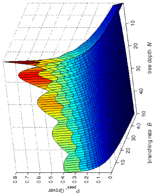
Figure 22: Variation of the first peak in the exit probability for branching rates up to $B=50$, and tree depths up to $N=50$ using a Grover coin operator.

The peak exit probability closely follows that of the continuous time walk scaling as $1/B$. Thus both continuous time and discrete Grover coined walks still beat a classical algorithm, which takes time proportional to the number of nodes, i.e. $T\sim B^{N}$, to find the exit with better than exponentially small exit probability. Combining the scalings for depth and branching rate, we have these two versions of quantum walks finding the exit in time linear in $N$ with probability proportional to $1/(BN^{2/3})$.

V.4 DFT coin operator on glued trees

We now consider the quantum walk with a DFT coin operator on the glued trees graph. The DFT coin operator does not have the right symmetry to map to a walk on the line for randomly applied coin labels, but if we apply a regular coin labeling that singles out the “root” direction to have coin label zero the mapping to the line can be carried out successfully. This is “cheating” as far as application to traversing the graph is concerned, since such a labeling would enable a classical algorithm to deterministically find the exit. Nonetheless, the branching trees that make up this graph appear widely in physics and computer science, so other applications that could use this regular labeling may arise. Note that the coin labeling in Tregenna et al. (2003) was consistent in that each end of each edge had the same label, but therefore could not always label the root direction as zero, and in fact made random label choices once the consistency condition was satisfied. Hence they did not find any advantage to using DFT coin over classical. With the regular labeling, the mapping works because the phase factors all neatly cancel out, as we now show. We start by assuming $C_{1}=C_{2}\dots=C_{B}=C$, and show that after applying the DFT coin operator as in equation (13) for $d=B+1$ we have $D_{1}=D_{2}\dots=D_{B}=D$. Thus if we start in a symmetric state, this will be preserved under the DFT coin operator. Using the notation in figure 20,

$$Q = \frac{1}{\sqrt{B+1}}\left\{P+BC\right\}$$

$$D_{1} = \frac{1}{\sqrt{B+1}}\left\{P+(\omega+\omega^{2}+\dots+\omega^{B})C\right\}$$

$$D_{2} = \frac{1}{\sqrt{B+1}}\left\{P+(\omega^{2}+\omega^{4}+\dots+\omega^{2B})C\right\}$$

$$\vdots$$

$$D_{B} = \frac{1}{\sqrt{B+1}}\left\{P+(\omega^{B}+\omega^{2B}+\dots+\omega^{B^{2}})C\right\}$$ (32)

where $\omega=e^{2\pi i/d}$ is the complex $d$’th root of unity. Each of the sums of powers of $\omega$ in the expressions for $D_{1}$ to $D_{B}$ evaluates to $-1$, hence we have $D_{1}=D_{2}\dots=D_{B}=D$ as claimed. Substituting for $P$, $Q$, $C$ and $D$ from equation (25) then gives

$$R_{O} = \sqrt{\frac{B}{B+1}}R_{I}-\frac{1}{\sqrt{B+1}}L_{I}$$

$$L_{O} = \frac{1}{\sqrt{B+1}}R_{I}+\sqrt{\frac{B}{B+1}}L_{I}$$ (33)

for the $2\times 2$ operator equivalent to the DFT coin operator. For $B\rightarrow\infty$, equation (33) becomes the identity, which corresponds to a walk that steps deterministically along the line, reaching the exit in the shortest possible time. For intermediate values of $B$, the DFT coined walk partly steps across the graph, and partly remains close to the entrance: an example is shown in figure 23 for a “glued trees” graph with branching rate $B=10$ and depth $N=10$.

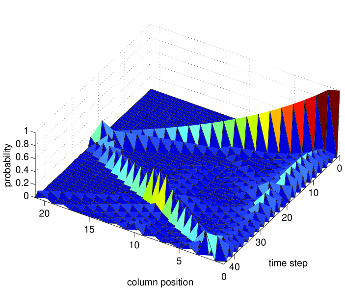
Figure 23: Propagation of the discrete quantum walk using the DFT coin operator on a glued trees graph for tree depth $N=10$ and branching rate $B=10$, run for 44 time steps.

Again we look at the first peak in the exit probability, which occurs after time $\sim(2N+2)$.

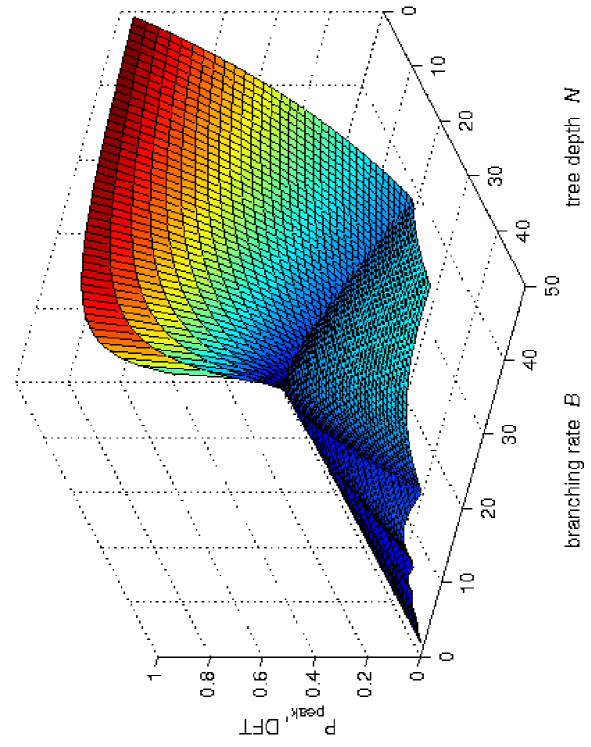
Figure 24: Variation of the first peak in the exit probability for branching rates up to $B=50$, and tree depths up to $N=50$ using a DFT coin operator.

The variation of this first peak in the probability with branching rate and tree depth for $N,B<50$ is plotted in figure 24. For $B=N$, there is a wide peak; on the $B>N$ side an initial peak rises towards unity, while on the $B<N$ side the probability tails off in a series of smaller arches. For $B=2$, the quantum walk with this coin operator has a noticeably lower probability of finding the exit after linear time than the Grover coin or the continuous time quantum walks. Nevertheless, there is still a peak in the probability of finding the walker at the exit, and our numerical results show this peak scales as $N^{-2/3}$, the same as the Grover coined walk and the continuous time walk, but with a constant prefactor $\sim 30$ times smaller.

We can understand this prefactor qualitatively as follows. The mapped-to-the-line version of the coined quantum walk is essentially a generalised Hadamard coin walk on finite line segments Bach et al. (2004). Such walks on the infinite line all have the typical double-peaked shape, with the ratio of the left and right peak heights determined by the coin biases and the initial state. The mapped-to-the-line versions of the Grover and regular DFT coins have the minus sign in opposite positions in the off-diagonal, equations (26) and (33). Combined with the rightward moving initial state, for the first half of the walk the largest peak is thus on the leading(trailing) edge for the Grover(DFT) coin operator. Moreover, the trailing edge DFT peak is larger than the leading edge Grover peak. For the second half of the walk the coin operators are transposed, and the trailing(leading) edge is largest for the Grover(DFT) coin operator, but this is combined with different “initial” states as the quantum walk crosses the glue from the first half of the walk, so the two effects don’t just cancel out. The cross-over point beyond which the regular DFT coin performs best is roughly $B>10$ for any tree depth.

VI Summary and Discussion

Even for the simple case of a coined quantum walk on the line we find that the entanglement between the coin and the particle position shows surprisingly rich behaviour. The entanglement oscillates around an asymptotic value that is determined by the bias in the coin operator, and the rate of convergence depends the symmetry in the distribution of the quantum walk, which in turn is determined by the initial state of the coin (assuming the quantum walk starts at the origin). More symmetric distributions (about the origin) converge faster than asymmetric distributions in which there is a bias favouring finding the particle in the positive or the negative half line.

For lattices in two spatial dimensions, similar rich patterns of behaviour are observed, the rate of convergence of the entanglement correlates with the extent to which the quantum walk spreads out over the grid, with fast convergence indicating good spreading behaviour, and slow convergence for distributions that bunch around one point, such as the origin. We find that for lattices in two spatial dimensions but of higher degree $d>4$, a DFT coin operator is better at spreading over the graph than a Grover coin operator. This can be explained by the bias in the Grover coin operator: above degree $d=4$, the Grover coin operator favours returning along the path it arrived from rather than picking a new direction, thus tending to keep the walk near where it started. The DFT coin operator is unbiased for any degree, so the spreading depends only on the relative phases, which can be controlled by the coin labeling.

For finite graphs, there are a few periodic examples, corresponding to those reported in Tregenna et al. (2003), otherwise the entanglement is random even for very simple cases, like the seven-cycle. A quantum walk on a complete bipartite graphs using a Grover coin operator is always periodic with period four, and we have shown this analytically. For the DFT coin, the quantum walk on complete bipartite graphs was not periodic for any cases we tested numerically.

For the glued trees graph and its generalisation to higher branching rates, the first peak in the probability for finding the quantum walker at the exit node occurs in linear time and scales with tree depth as $N^{-2/3}$ for both Grover and DFT coin operators, matching that found for the continuous time walk by Childs et al. Childs et al. (2003). This is in contrast with classical algorithms, which require exponential time to find the exit with better than exponentially small probability. However, for increased branching rate, while the continuous time walk and the Grover coined discrete time walk both scale as $B^{-1}$, a DFT coin with regular coin labels has a success probability approaching unity for $B>N>>1$, and beats the continuous time and Grover coined walks for $B\gtrsim 10$. A regular coin labeling is not permitted in the algorithmic context of Childs et al. (2003), but branching trees occur in many other contexts, some of which may permit a regular coin labeling such that this DFT coin property could prove useful.

Another observation from this work is that since the coin needs to have as many dimensions as the maximum degree of the graph, it allows a relative phase to be introduced at vertices of less than the maximum degree, for example, at the entrance and exit of the “glued trees” graph, see figure 21. The quantum walk may exhibit different properties depending on the choice of relative phase, which provides extra options for tuning the quantum walk.

Overall, the discrete quantum walk offers many options for tuning the properties of the quantum coin operator to fit the problem to be solved. These possibilities are not available in the continuous time quantum walk, unless one adds extra degrees of freedom Childs and Goldstone (2004b) (whereupon it becomes exactly equivalent). Further work could investigate how to optimise the uniformity of spreading over these higher dimensional lattices, for example, by applying small amounts of decoherence (see Tregenna et al. (2003)) and by adjusting the coin operator: we do not know whether the DFT coin operator is the optimal choice for a general $d$-dimensional graph for $d>4$.