Semiclassical propagation of coherent states using complex and real trajectories

Abstract

A semiclassical approximation to the time evolution of coherent states may be derived from a saddle point approximation to the exact quantum propagator, and in general it involves complex classical dynamics. We generalize previous one-dimensional results to $d$ dimensions, and for the case $d=2$ we present several applications. We also consider other simple approximations that depend only on real classical trajectories, but are not initial value representations. These approximations are able to reproduce interference and tunnelling effects, and involve propagating a few classical initial conditions compatible with the quantum uncertainties.

I Introduction

Semiclassical propagators involving complex classical trajectories in real time have appeared in the coherent states representation around 25 years ago klauder ; weiss . A stationary phase approximation to the transition amplitude $\langle z^{\prime}|e^{-iHT/\hbar}|z\rangle$, where $|z\rangle$ is a coherent state, leads to trajectories satisfying the usual Hamilton equations subject to special boundary conditions that can only be satisfied in a complexified phase space. Numerical calculations in this representation have been done both for chaotic systems adachi ; cabelo and for one dimensional systems marcus ; xavier ; parisio (see also voorhis ; reviews can be found in rubin ; baranger ). Semiclassical calculations involving complex trajectories in the mixed representation $\langle x|e^{-iHT/\hbar}|z\rangle$, on the other hand, were introduced in huber and recently rediscovered aguiar for the one-dimensional case (see boiron for a different approach). Since the mixed representation is the most interesting for the propagation of wave packets, our purpose here is to generalize this formalism to many dimensions and to present some applications.

The calculation of complex trajectories involves two difficulties: first, the effective dimensionality of the phase space is doubled, since both real and imaginary parts of position and momenta have to be computed; second, the trajectories must satisfy mixed boundary conditions, part at the initial time and part at the final time, a problem known as ‘root search’. Therefore we also consider the possibility of employing only real trajectories in the semiclassical approximation. This is done by approximating the complex trajectories by real ones, satisfying modified boundary conditions that are less restrictive than the original ones. Although such real trajectories approximations are always less accurate than the original complex one, they are much simpler and sometimes have practically the same accuracy aguiar . Our approach, both with complex and real trajectories, does not involve integrations over initial conditions, a procedure that is common to IVR – Initial Value Representations (recent reviews of this method can be found in review ). IVR methods are usually easy to apply and reasonably accurate for long times. Nevertheless, for short times the present method provides a much clearer physical picture since only a few families of trajectories are required.

We start from a coherent state $|{\bf z}\rangle$, where

$${\bf z}=\frac{1}{\sqrt{2}}\left(B^{-1}{\bf q}+iC^{-1}{\bf p}\right),$$ (1)

and the $d$-dimensional vectors ${\bf q}$ and ${\bf p}$ are the average values of position and momentum for this state. The diagonal matrices $B$ and $C$ contain the position and momentum uncertainties, respectively, and satisfy the condition $B=\hbar C^{-1}$. The position representation of this coherent state is a Gaussian,

$$\langle{\bf x}|{\bf z}\rangle=\mathcal{N}\exp\left\{\frac{i}{\hbar}{\bf p}^{T}({\bf x}-{\bf q})-\frac{1}{2}({\bf x}-{\bf q})^{T}B^{-2}({\bf x}-{\bf q})\right\},$$ (2)

where $\mathcal{N}=|B|^{-\frac{1}{2}}\pi^{-\frac{d}{4}}$ (we use the symbol $|\cdot|$ for the determinant). After a time $T$, the propagated wave function is given by

$$\psi({\bf x},T)=\langle{\bf x}|K(T)|{\bf z}\rangle,$$ (3)

where $K(T)=e^{-iHT/\hbar}$.

In order to calculate the wave function semiclassically we shall follow the procedure of huber ; aguiar . We first insert in (3) a resolution of unity to obtain

$$\psi({\bf x},T)=\int d{\bf x}^{\prime}\langle{\bf x}|K(T)|{\bf x}^{\prime}\rangle\langle{\bf x}^{\prime}|{\bf z}\rangle,$$ (4)

and substitute the quantity $\langle{\bf x}|K(T)|{\bf x}^{\prime}\rangle$ by its semiclassical Van-Vleck expression vleck ; gutzwiller . Then we make the integration by the stationary exponent approximation. We shall see that the stationary points are in general complex numbers, and thus a deformation of the integration contour into the complex plane is unavoidable, taking the classical trajectories involved in the approximation to a complex phase space.

The Van-Vleck formula in $d$ dimensions is

$$\langle{\bf x}|K(T)|{\bf x}^{\prime}\rangle_{VV}=(2\pi i\hbar)^{-d/2}\sqrt{\left|-S_{{\bf x}{\bf x}^{\prime}}\right|}e^{\frac{i}{\hbar}S},$$ (5)

where $S({\bf x},{\bf x}^{\prime},T)$ is the action of the classical trajectory that goes from ${\bf x}^{\prime}$ to ${\bf x}$ in time $T$ and $S_{{\bf x}{\bf x}^{\prime}}$ is the matrix of its second derivatives (we have incorporated Morse phases in $S$). If more than one such trajectory exists, one should sum their contributions. Before performing the integration, let us express the determinant in (5) in terms of the elements of the tangent matrix. As shown in the appendix,

$$\langle{\bf x}|K(T)|{\bf x}^{\prime}\rangle_{VV}=\frac{(2\pi i)^{-d/2}}{|B|\sqrt{|M_{{\bf x}{\bf p}}|}}e^{\frac{i}{\hbar}S}.$$ (6)

Note that in the position representation nothing is said about the momentum of the corresponding classical trajectory, and therefore it is not necessary to introduce any complexification. In the coherent states representation the boundary conditions are too stringent as one tries to specify not only the initial and final points (and the time) but also the initial and final momenta baranger .

In the next section we shall calculate the integral (4) in the saddle point approximation, valid in the semiclassical limit. In section III we develop further approximations that involve only real classical trajectories. We show some illustrative numerical applications in section IV and present our conclusions in section V.

II Complex trajectories

In the semiclassical limit the wave function in (4) can be written as

$$\psi({\bf x},T)=\frac{\mathcal{N}}{|B|}(2\pi i)^{-d/2}\int d{\bf x}^{\prime}\frac{\exp\{\frac{i}{\hbar}\Phi({\bf x},{\bf x}^{\prime},T)\}}{\sqrt{|M_{{\bf x}{\bf p}}|}},$$ (7)

where

$$\frac{i}{\hbar}\Phi=\frac{i}{\hbar}[S+{\bf p}^{T}({\bf x^{\prime}}-{\bf q})]-\frac{1}{2}({\bf x^{\prime}}-{\bf q})^{T}B^{-2}({\bf x^{\prime}}-{\bf q}).$$ (8)

We evaluate this integral by the usual saddle point method, which consists in expanding the exponent to second order around its stationary point ${\bf x}^{\prime}_{0}$, while the prefactor is simply evaluated at this point. After performing the resulting Gaussian integration, this leads to the semiclassical approximation

$$\psi_{\rm sc}({\bf x},T)=\frac{\mathcal{N}}{|B|}(2\pi i)^{-d/2}\frac{\exp\{\frac{i}{\hbar}\Phi_{0}\}}{\sqrt{|M_{{\bf x}{\bf p}}|}}\sqrt{-\frac{(2\pi)^{d}}{|\Phi_{{\bf x}^{\prime}{\bf x}^{\prime}}|}},$$ (9)

where

$$\Phi_{{\bf x}^{\prime}{\bf x}^{\prime}}=\frac{i}{\hbar}S_{{\bf x}^{\prime}{\bf x}^{\prime}}-B^{-2}$$ (10)

and $\Phi_{0}=\Phi({\bf x},{\bf x}^{\prime}_{0},T)$.

The stationary point ${\bf x}^{\prime}_{0}$, determined imposing the condition $\left.\nabla^{\prime}\Phi\right|_{{\bf x}^{\prime}_{0}}=0$, is given by

$$B^{-1}({\bf x}^{\prime}_{0}-{\bf q})=iC^{-1}({\bf p}-{\bf p}^{\prime}_{0}),$$ (11)

where ${\bf p}^{\prime}_{0}({\bf x},{\bf x}^{\prime}_{0},T)=-\left.\nabla^{\prime}S\right|_{{\bf x}^{\prime}_{0}}$. Both ${\bf p}^{\prime}_{0}$ and ${\bf x}^{\prime}_{0}$ are in general complex numbers, and the whole classical trajectory therefore takes place in a complex phase space. It leaves ${\bf x}^{\prime}_{0}$ at time $0$ with the complex momentum ${\bf p}^{\prime}_{0}$ and arrives at the real position ${\bf x}$ at time $T$. The classical action $S$ and the tangent matrix $M$ will also be complex in general.

Using the relation (see appendix)

$$|\Phi_{{\bf x}^{\prime}{\bf x}^{\prime}}|=\frac{i^{d}}{|B|^{2}}\frac{|M_{{\bf x}{\bf x}}+iM_{{\bf x}{\bf p}}|}{|M_{{\bf x}{\bf p}}|},$$ (12)

the final result may be written in terms of the tangent matrix as

$$\psi_{\rm sc}({\bf x},T)=\frac{\mathcal{N}(-i)^{d-1}}{\sqrt{|M_{{\bf x}{\bf x}}+iM_{{\bf x}{\bf p}}|}}\exp\{\frac{i}{\hbar}\Phi_{0}\}.$$ (13)

This generalizes the one dimensional formula presented in huber ; aguiar , to which it reduces for separable systems and that has proven to be accurate in the evolution of wave packets in many different systems. It is of course exact for the propagation of a $d$-dimensional coherent state in free space and in potentials up to quadratic (harmonic oscillator, charged particle in constant electromagnetic/grativational field). Differently from the Van Vleck approximation, the prefactor involves the square root of a complex number (remember that $|\cdot|$ is a determinant, not a modulus), and its phase must be determined dynamically with the condition that for $T=0$ we have $M_{{\bf x}{\bf x}}=1$ and $M_{{\bf x}{\bf p}}=0$.

The semiclassical approximation (13) depends on complex trajectories $({\bf q}(t),{\bf p}(t))$ satisfying the boundary conditions

$$\frac{1}{\sqrt{2}}\left(B^{-1}{\bf q}(0)+iC^{-1}{\bf p}(0)\right)={\bf z},\quad\quad{\bf q}(T)={\bf x},$$ (14)

where we have used the fact that (11) can be written $B^{-1}{\bf x}^{\prime}_{0}+iC^{-1}{\bf p}^{\prime}_{0}=B^{-1}{\bf q}+iC^{-1}{\bf p}$. The final value of the momentum is not restricted and will be complex in general. Following Klauder and Adachi klauder ; rubin ; adachi we may write the initial condition as

$${\bf q}(0)={\bf q}+{\boldsymbol{\omega}},\quad{\bf p}(0)={\bf p}+iCB^{-1}{\boldsymbol{\omega}},$$ (15)

where ${\boldsymbol{\omega}}={\boldsymbol{\alpha}}+i{\boldsymbol{\beta}}$ is a complex vector to be determined. The first condition is automatically satisfied for any ${\boldsymbol{\omega}}$. For a fixed time $T$ the propagation of this complex initial condition defines a complex map ${\boldsymbol{\omega}}\to{\bf q}(T)$, the properties of which have been studied in detail for the one-dimensional case in rubin . Only for some values of ${\boldsymbol{\omega}}$ will it happen that ${\bf q}(T)\in\mathbb{R}^{d}$, and we denote the set of all those points by $\Omega$. It is easy to see that ${\boldsymbol{\omega}}=0$ belongs to $\Omega$, in which case we have the classical trajectory of the center of the wave packet.

However, the inverse of the map ${\boldsymbol{\omega}}\to{\bf q}(T)$ is in general globally multivalued: there may be many trajectories that end at the same ${\bf q}(T)$. Therefore $\Omega$ will consist in a finite collection of $d$-dimensional disjoint sets, called families. In the vicinity of a critical point (i.e., one for which $\partial{\bf q}(T)/\partial{\boldsymbol{\omega}}$ is zero) the map is two-to-one, provided the second derivative is not zero. Such a critical point is also called a phase space caustic. At these points $|M_{{\bf x}{\bf x}}+iM_{{\bf x}{\bf p}}|\to 0$, thus preventing the validity of the semiclassical calculation. It is possible to develop a semiclassical approximation based on the Airy function that remains valid near caustics. For the one-dimensional case this has been derived in uniform .

The family of trajectories that contains the point ${\boldsymbol{\omega}}=0$ is called the main family, and it provides the most important contribution to the semiclassical approximation. As time increases, other families may become relevant. The imaginary part of $\Phi_{0}$ is positive for all trajectories that belong to the main family, but this may not be the case for other families. When $\rm{Im}(\Phi_{0})<0$ one has a contribution that diverges when $\hbar\to 0$ and therefore must be discarded. These are called non-contributing trajectories, and for some families it is necessary to introduce a cut-off in order to avoid them.

Another delicate point is that of Stokes lines and exponential dominance, which is intrinsic to many asymptotic formulations. In the usual one-dimensional WKB, for example, the semiclassical approximation for stationary states becomes singular at classical turning points, and one must connect different local solutions by an analytic continuation. In so doing, one finds that there must be a change in the number of contributions along certain lines called Stokes lines stokes ; dingle ; berry ; shudo . In the vicinity of such a line one contribution dominates exponentially over the other, and one is free to place a cut-off (the error due to the cut-off is less than the error due to the semiclassical approximation). The same phenomenon appears in the present formalism. Even though the location of these lines is hard to determine in principle, in practice when crossing them there appears a false divergence in the approximation, which can be easily detected aguiar .

III Approximations based on real trajectories

One may wish to find approximations for the expression (13) that involve only real trajectories. There are many such possibilities. One possible choice is the trajectory that starts at the real point ${\bf q}$ with initial momentum ${\bf p}_{i}$, different from ${\bf p}$, and after a time $T$ arrives at ${\bf x}$. Another possibility is a trajectory that starts with momentum ${\bf p}$ but from a different point ${\bf q}_{i}$ and also arrives at ${\bf x}$. We can also give up the final point condition, for example, by choosing the unique trajectory that starts at ${\bf q}$ with momentum ${\bf p}$. All these possibilities are similar to the ones already existent in the one-dimensional case aguiar , but in more dimensions one can in principle come up with others. For example, in two dimensions a trajectory may exist that starts at $(q_{x},q_{yi})$ with momentum $(p_{xi},p_{y})$ and ends at $(x,y)$, but with $q_{yi}\neq q_{y}$ and $p_{xi}\neq p_{x}$. All these real trajectories should be good approximations for the complex stationary trajectory if the latter is not too deep into the complex plane.

An important method that is also based on real trajectories is the ‘cellular dynamics’, developed by Heller cellular ; houches , in which a grid of initial conditions is evolved and each contribution to the propagator is obtained by a linearization of the dynamics. This method was initially used to propagate wave packets cellular and later to obtain coherent state correlation functions $\langle z^{\prime}|e^{-iHT/\hbar}|z\rangle$ in chaotic systems celchaos1 ; celchaos2 . The calculations we present in this section are close in spirit to these works, but instead of following the ‘cellular’ approach we start from the complex trajectory approximation (13), and we also consider a variety of boundary conditions that the real trajectories may satisfy. Using different boundary conditions we obtain the ‘central’ trajectory approximation houches and also more general results similar to the ‘off-centered’ one presented in celchaos2 .

This section regards only calculation of wave functions, but a discussion of the quantity $\langle z^{\prime}|e^{-iHT/\hbar}|z\rangle$ that proceeds along the same lines may be found in realzz .

III.1 Approximation via central trajectory

The classical trajectory that starts at $({\bf q},{\bf p})$ will end, after a time $T$, in the point $({\bf q}_{r},{\bf p}_{r})$. Following aguiar we write

$${\bf x}^{\prime}_{0} = {\bf q}+\Delta{\bf x}^{\prime}$$ (16)

$${\bf p}^{\prime}_{0} = {\bf p}+\Delta{\bf p}^{\prime}={\bf p}-S_{{\bf x}^{\prime}{\bf x}^{\prime}}\Delta{\bf x}^{\prime}-S_{{\bf x}^{\prime}{\bf x}}\Delta{\bf x}$$ (17)

$${\bf x} = {\bf q}_{r}+\Delta{\bf x}$$ (18)

$${\bf p} = {\bf p}_{r}+\Delta{\bf p}={\bf p}_{r}+S_{{\bf x}{\bf x}^{\prime}}\Delta{\bf x}^{\prime}+S_{{\bf x}{\bf x}}\Delta{\bf x}.$$ (19)

The stationary exponent condition can be written as $\Delta{\bf p}^{\prime}=i\hbar B^{-2}\Delta{\bf x}^{\prime}$, and equation (17) can be solved to give (see appendix)

$$\Delta{\bf x}^{\prime}=B(M_{{\bf x}{\bf x}}+iM_{{\bf x}{\bf p}})^{-1}B^{-1}\Delta{\bf x}.$$ (20)

Now we expand the exponent in (13) around this trajectory to second order in $\Delta{\bf x}$. The expansion of the action is

$$S\simeq S_{r}+ {\bf p}_{r}^{T}\Delta{\bf x}-{\bf p}^{T}\Delta{\bf x}^{\prime}$$

$$+\frac{1}{2}(\begin{array}[]{cc}\Delta{\bf x}&\Delta{\bf x}^{\prime}\end{array})\begin{pmatrix}S_{{\bf x}{\bf x}}&S_{{\bf x}{\bf x}^{\prime}}\\ S_{{\bf x}^{\prime}{\bf x}}&S_{{\bf x}^{\prime}{\bf x}^{\prime}}\end{pmatrix}\left(\begin{array}[]{c}\Delta{\bf x}\\ \Delta{\bf x}^{\prime}\end{array}\right).$$ (24)

The remaining terms are simply ${\bf p}^{T}\Delta{\bf x}^{\prime}$, which cancels out, and $\Delta{\bf x}^{\prime T}B^{-2}\Delta{\bf x}^{\prime}$. In the quadratic terms we introduce the tangent matrix and use (20) to obtain

$$\psi_{{\bf q}{\bf p}}({\bf x},T)=\frac{\mathcal{N}(-i)^{d-1}}{\sqrt{|M_{{\bf x}{\bf x}}+iM_{{\bf x}{\bf p}}|}}\exp\{\frac{i}{\hbar}\Phi_{r}\},$$ (25)

where the exponent is given by (see appendix)

$$\frac{i}{\hbar}\Phi_{r}=\frac{i}{\hbar}(S_{r}+{\bf p}_{r}^{T}\Delta{\bf x})-\frac{1}{2}\Delta{\bf x}B^{-1}\Xi B^{-1}\Delta{\bf x},$$ (26)

where $\Xi=(M_{{\bf p}{\bf p}}-iM_{{\bf p}{\bf x}})(M_{{\bf x}{\bf x}}+iM_{{\bf x}{\bf p}})^{-1}$. Note that this is always Gaussian in $\Delta{\bf x}$, with variable width. Therefore this approximation can never account for interferences or tunnelling effects. Notice that while the formula (13) involves an infinite number of classical trajectories, at least one for each value of ${\bf x}$, the one we just derived requires only the trajectory that starts in $({\bf q},{\bf p})$. For this reason this is called an Initial Value Representation (IVR).

This formula was first derived by Heller heller (see also houches ) and is called the Thawed Gaussian Approximation or TGA (it was rederived with some detail in baranger ). It becomes exact in the semiclassical limit $\hbar\to 0$ (for a fixed value of time) and has been used, for example, in the study of decoherence fiete and of scars in quantum chaotic systems scars . In the applications presented here we are interested in quantum effects that cannot be reproduced by the TGA, and thus we do not consider it any further.

III.2 Approximation via trajectory ${\bf q}\to{\bf x}$

Let us fix the initial coordinate of the trajectory, ${\bf q}$, and demand that after a time $T$ it arrives at ${\bf x}$. We need to find the initial momentum ${\bf p}_{i}$ for such trajectories, and in fact there may be more than one that satisfy the above conditions. We write

$${\bf x}^{\prime}_{0} = {\bf q}+\Delta{\bf x}^{\prime}$$ (27)

$${\bf p}^{\prime}_{0} = {\bf p}_{i}+\Delta{\bf p}^{\prime}={\bf p}_{i}-S_{{\bf x}^{\prime}{\bf x}^{\prime}}\Delta{\bf x}^{\prime}.$$ (28)

Note that the complete expansion of ${\bf p}^{\prime}_{0}$ to first order should be ${\bf p}_{i}-S_{{\bf x}^{\prime}{\bf x}^{\prime}}\Delta{\bf x}^{\prime}-S_{{\bf x}^{\prime}{\bf x}}\Delta{\bf x}$, but we are keeping ${\bf x}$ fixed.

Equation (11) gives

$$B^{-1}\Delta{\bf x}^{\prime}=iC^{-1}(\Delta{\bf p}-\Delta{\bf p}^{\prime}),$$ (29)

where $\Delta{\bf p}={\bf p}-{\bf p}_{i}$. Using (28) we find

$$(\frac{i}{\hbar}S_{{\bf x}^{\prime}{\bf x}^{\prime}}-B^{-2})\Delta{\bf x}^{\prime}=\Phi_{{\bf x}^{\prime}{\bf x}^{\prime}}\Delta{\bf x}^{\prime}=-\frac{i}{\hbar}\Delta{\bf p},$$ (30)

which we can invert to write

$$\Delta{\bf x}^{\prime}=-\frac{i}{\hbar}\Phi_{{\bf x}^{\prime}{\bf x}^{\prime}}^{-1}\Delta{\bf p}.$$ (31)

We now expand the exponent in (13) around this trajectory to second order in $\Delta{\bf x}^{\prime}$. Proceeding analogously to the one-dimensional case aguiar we obtain

$$\frac{i}{\hbar}\Phi_{{\bf q}}=\frac{i}{\hbar}S_{{\bf q}}+\frac{1}{2\hbar^{2}}\Delta{\bf p}^{T}\Phi_{{\bf x}^{\prime}{\bf x}^{\prime}}\Delta{\bf p},$$ (32)

which, with a few algebraic manipulations, may be expressed in terms of the tangent matrix (see appendix) as

$$\frac{i}{\hbar}\Phi_{{\bf q}}=\frac{i}{\hbar}S_{{\bf q}}-\frac{i}{2}\Delta{\bf p}^{T}C^{-1}(M_{{\bf x}{\bf x}}+iM_{{\bf x}{\bf p}})^{-1}M_{{\bf x}{\bf p}}C^{-1}\Delta{\bf p}.$$ (33)

The wave function becomes

$$\psi_{\bf q}({\bf x},T)=\frac{\mathcal{N}(-i)^{d-1}}{\sqrt{|M_{{\bf x}{\bf x}}+iM_{{\bf x}{\bf p}}|}}\exp\{\frac{i}{\hbar}\Phi_{\bf q}\}.$$ (34)

The exponent contains the real action $S_{\bf q}$ and a term which is Gaussian in the difference between ${\bf p}_{i}$, the initial momentum of the trajectory, and ${\bf p}$, the average momentum of the initial coherent state. It is important to note that ${\bf p}_{i}$ usually depends on ${\bf x}$ in a complicated manner, and thus the final wave packet will not, in general, be Gaussian. Also, there may exist more than one value of ${\bf p}_{i}$, and a sum over all possible trajectories would be required, resulting in interference terms. Since the trajectory involved in the calculation depends on the initial ${\bf q}$ and final ${\bf x}$ points, this is not an IVR.

III.3 Approximation via trajectory ${\bf p}\to{\bf x}$

We now fix the initial momentum of the trajectory and allow it to start from a point ${\bf q}_{i}$ that is different from the center of the wave packet. We write

$${\bf x}^{\prime}_{0} = {\bf q}_{i}+\Delta{\bf x}^{\prime}$$ (35)

$${\bf p}^{\prime}_{0} = {\bf p}+\Delta{\bf p}^{\prime}={\bf p}-S_{{\bf x}^{\prime}{\bf x}^{\prime}}\Delta{\bf x}^{\prime},$$ (36)

and use the stationary exponent condition (11) to find

$$(\frac{i}{\hbar}S_{{\bf x}^{\prime}{\bf x}^{\prime}}-B^{-2})\Delta{\bf x}^{\prime}=-B^{-2}\Delta{\bf q}$$ (37)

or $\Delta{\bf x}^{\prime}=-\Phi_{{\bf x}^{\prime}{\bf x}^{\prime}}^{-1}B^{-2}\Delta{\bf q}$, with $\Delta{\bf q}={\bf q}-{\bf q}_{i}$. Once again, we expand the exponent in (13) to second order in $\Delta{\bf x}^{\prime}$, but this time we write it in terms of $\Delta{\bf q}$. The final result is

$$\psi_{\bf p}({\bf x},T)=\frac{\mathcal{N}(-i)^{d-1}}{\sqrt{|M_{{\bf x}{\bf x}}+iM_{{\bf x}{\bf p}}|}}\exp\{\frac{i}{\hbar}\Phi_{\bf p}\},$$ (38)

where

$$\frac{i}{\hbar}\Phi_{\bf p} =\frac{i}{\hbar}(S_{\bf p}-{\bf p}^{T}\Delta{\bf q})$$

$$-\frac{1}{2}\Delta{\bf q}^{T}B^{-1}(M_{{\bf x}{\bf x}}+iM_{{\bf x}{\bf p}})^{-1}M_{{\bf x}{\bf x}}B^{-1}\Delta{\bf q}.$$ (39)

We have obtained a Gaussian again, this time in the difference between ${\bf q}_{i}$, the initial position of the trajectory, and ${\bf q}$, the average position of the initial coherent state. This is again not an IVR, and after a time $T$ it will not result in a Gaussian in ${\bf x}$. It may as well display interference between different existent classical trajectories.

III.4 Approximation via a mixed trajectory

We now restrict ourselves to a two-dimensional system and choose the real trajectory that starts at $(q_{x},q_{yi})$ with momentum $(p_{xi},p_{y})$ and ends at $(x,y)$, but with $q_{yi}\neq q_{y}$ and $p_{xi}\neq p_{x}$. This time we have mixed conditions, and we set

$$x^{\prime}_{0} = q_{x}+\Delta x^{\prime},$$ (40)

$$y^{\prime}_{0} = q_{yi}+\Delta y^{\prime},$$ (41)

$$p^{\prime}_{x0} = p_{xi}+\Delta p^{\prime}_{x}=p_{xi}-S_{x^{\prime}x^{\prime}}\Delta x^{\prime}-S_{x^{\prime}y^{\prime}}\Delta y^{\prime},$$ (42)

$$p^{\prime}_{y0} = p_{y}+\Delta p^{\prime}_{y}=p_{y}-S_{y^{\prime}x^{\prime}}\Delta x^{\prime}-S_{y^{\prime}y^{\prime}}\Delta y^{\prime}.$$ (43)

Using these equations, the stationarity conditions can be cast in the form $\Delta{\bf x}^{\prime}=-\Phi_{{\bf x}^{\prime}{\bf x}^{\prime}}^{-1}\Delta{\boldsymbol{\xi}}$, where

$$\Delta{\boldsymbol{\xi}}=\begin{pmatrix}i\Delta p_{x}/\hbar\\ \Delta y/b_{y}^{2}\end{pmatrix},\quad\Delta{\bf x}^{\prime}=\begin{pmatrix}\Delta x^{\prime}\\ \Delta y^{\prime}\end{pmatrix}.$$ (44)

The expansion of the exponent to second order in $\Delta{\bf x}^{\prime}$ is $S\approx S_{M}+\nabla^{\prime}S^{T}\Delta{\bf x}^{\prime}+\frac{1}{2}\Delta{\bf x}^{\prime T}S_{x^{\prime}x^{\prime}}\Delta{\bf x}^{\prime}$ for the action, ${\bf p}^{T}({\bf x}^{\prime}_{0}-{\bf q})=-\nabla^{\prime}S^{T}\Delta{\bf x}^{\prime}-p_{y}\Delta y$ for the term involving the wave packet momentum and $({\bf x}^{\prime}_{0}-{\bf q})^{T}B^{-2}({\bf x}^{\prime}_{0}-{\bf q})=\Delta{\bf x}^{\prime T}B^{-2}\Delta{\bf x}^{\prime}+b_{y}^{-2}\Delta y(\Delta y-2\Delta y^{\prime})$ for the quadratic term. The linear terms in $\Delta{\bf x}^{\prime}$ cancel, and after we change from $\Delta{\bf x}^{\prime}$ to $\Delta\xi$ we have

$$\frac{i}{\hbar}\Phi_{M}=\frac{i}{\hbar}(S_{M}-p_{y}\Delta y)-\frac{1}{2}\Delta\xi^{T}\Phi^{-1}_{{\bf x}^{\prime}{\bf x}^{\prime}}\Delta\xi-\frac{\Delta y^{2}}{2b_{y}^{2}},$$ (45)

where $S_{M}$ is the action for the mixed condition trajectories. Once again this can be written in terms of the tangent matrix, as we show in the appendix. The wave function becomes

$$\psi_{M}(x,y,T)=\frac{-i}{\sqrt{\pi b_{x}b_{y}}}\frac{\exp\{\frac{i}{\hbar}\Phi_{M}\}}{\sqrt{|M_{{\bf x}{\bf x}}+iM_{{\bf x}{\bf p}}|}}.$$ (46)

III.5 Alternative derivation

Given the integral in (7) one may argue that, if the position uncertainties are very small, only the region around ${\bf q}$ will be relevant for the integration. Expanding the action to second order around this point we have

$$\frac{i}{\hbar}\Phi\approx \frac{i}{\hbar}S({\bf x},{\bf q})-\frac{i}{\hbar}({\bf p}_{i}-{\bf p})^{T}({\bf x}^{\prime}-{\bf q})$$

$$+\frac{1}{2}({\bf x}^{\prime}-{\bf q})^{T}\Phi_{{\bf x}^{\prime}{\bf x}^{\prime}}({\bf x}^{\prime}-{\bf q}),$$ (47)

where ${\bf p}_{i}=-\left.\nabla^{\prime}S\right|_{{\bf x}^{\prime}={\bf q}}$ is the initial momentum, generally different from ${\bf p}$. Proceeding with the integration, we find the same result as in section V.A, which is based on the trajectory that starts at ${\bf q}$ with momentum ${\bf p}_{i}$ and ends at ${\bf x}$ with any momentum at time $T$.

Jalabert and Pastawski jalabert have used a similar argument in their treatment of the quantum fidelity

$$\int\psi^{\ast}({\bf x},T)\psi_{V}({\bf x},T)d{\bf x},$$ (48)

(in this equation $\psi({\bf x},T)$ and $\psi_{V}({\bf x},T)$ are obtained from an initial wave function by evolving it with two different Hamiltonians), but they expanded the action to first order in the difference ${\bf x}^{\prime}-{\bf q}$ (the same procedure was used in petitjean ). After changing the integration variable in (48) from ${\bf x}$ to ${\bf p}_{i}$, Vanicek and Heller vanicek arrive at a semiclassical result that is free of caustics. Even though expanding the action to first order only is inaccurate for simple systems such as the free particle and the harmonic oscillator, their final formula seems to work well in practice. The expansion to second order we just presented is in principle more accurate, but the result it gives for the semiclassical fidelity is sensitive to caustics and thus probably less stable in numerical calculations.

Finally we note that, if instead of inserting a position representation of unity in (3), we used a momentum representation,

$$\psi({\bf x},T)=\int d{\bf p}^{\prime}\langle{\bf x}|K(T)|{\bf p}^{\prime}\rangle\langle{\bf p}^{\prime}|{\bf z}\rangle,$$ (49)

then after a similar second order expansion of the action, this time around ${\bf p}^{\prime}={\bf p}$, we would arrive at the expression (38) for the wave function. This is justified when the momentum uncertainties are small. The TGA approximation can also be obtained this way: one must enforce a stationary phase condition on the imaginary part of $\Phi({\bf x},{\bf x}^{\prime})$ alone.

IV Applications

In this section we present a few numerical applications of the approximations we have just derived. We compare the complex-trajectories formula (13) with the ones based on real trajectories, and also with exact quantum mechanical calculations, which we have carried out using Fast Fourier Transform methods. The purpose here is not to obtain extremely accurate numerical results, even though sometimes this is the case, but rather to illustrate the usefulness of semiclassical calculations in many different situations.

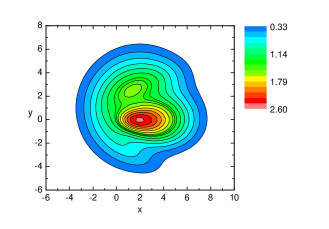
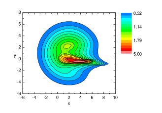
Figure 1: (color online) Exact (up) and semiclassical (down) probability densities (times $10^{2}$) at $T=4$, with ${\bf q}=(-10,1)$ and ${\bf p}=(3,0)$, in the case of an attractive Gaussian potential. Except for the main peak (notice the change in scale), the wave function is accurately reproduced, and $|\langle\psi|\psi_{\rm sc}\rangle|^{2}\approx 92\%$

IV.1 Attractive Gaussian potential

We start by investigating the semiclassical propagation in a two dimensional attractive Gaussian potential,

$$V(r)=-e^{-r^{2}},$$ (50)

where $r^{2}=x^{2}+y^{2}$. A one dimensional version of this problem was already considered in aguiar , where the semiclassical approximation was shown to be very accurate. This potential is also interesting because, unless the particle’s momentum is very low (which is not the case we are interested in), there is only one classical trajectory that contributes to the real semiclassical formulas presented in sections III-A to III-D. In the complex case there may be more than one trajectory, but we will confine ourselves to the main family only, since it already gives a very good result.

We place the wave packet initially at ${\bf q}=(-10,1)$, and chose $b_{x}=b_{y}=1$, so that the impact parameter is equal to the wave packet width. After a time interval of $t=4$ the main peak has followed a curved trajectory, arriving at a negative value of $y$, and a smaller peak appears around $y\approx 2$, as we can see in Fig 1a. This is accurately reproduced by the semiclassical approximation $\psi_{\rm sc}({\bf x},t)$, shown in Fig. 1b. The secondary peak is recovered almost exactly, but the height of the main peak is wrong by a factor of $2$ (notice the particular scale that has been used). The phase of the wave function is also recovered, and in fact the overlap

$$|\langle\psi|\psi_{\rm sc}\rangle|^{2}$$ (51)

is around $92\%$. It is important to notice that the discrepancy comes from a small region around the peak, and that the functions agree very well at all other points. We have also calculated the real trajectory approximations $\psi_{{\bf q}}({\bf x},t)$, $\psi_{{\bf p}}({\bf x},t)$ and $\psi_{M}({\bf x},t)$, but none of them can be distinguished from the complex one at this scale.

The erroneous increase in the main peak is probably due to the presence of a caustic in complex phase space. Even though only one real trajectory exists, in the complex case there may be more than one, leading to critical points in the map described in section II. In order to obtain a better approximation in the vicinity of the peak, either a uniform approximation or incorporation of this secondary family of trajectories would be necessary. Finding these trajectories in practice is the notorious root-search problem, known to be very difficult in more than one dimension. The accuracy of the simpler formulas (34), (38) and (46) in this case shows that they can be of practical use.

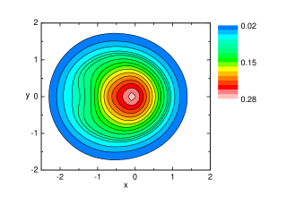
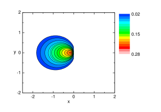
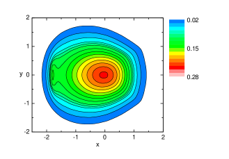
Figure 2: (color online) Probability density at $T=2.4$ for the quartic oscillator, with ${\bf q}=(0,0)$ and ${\bf p}=(2,0)$. The upper panel shows the exact calculation, the middle one is $|\psi_{\bf q}(x,y)|^{2}$ and the lower one is $|\psi_{\rm sc}(x,y)|^{2}$. Using only real trajectories the result is very poor, but it becomes excellent when complex ones are used: the overlap (51) in this case is around $95\%$.

IV.2 A bound system

We now study a bound system, an isotropic quartic oscillator:

$$V(r)=Ar^{2}+Br^{4},$$ (52)

where $A=0.5$ and $B=0.1$. The initial wave packet has parameters $b_{x}=b_{y}=1$, ${\bf q}=(0,0)$ and ${\bf p}=(2,0)$, which corresponds to a classical initial condition that is periodic with period $\tau\approx 4.7$. In Fig. 2a we show the probability density at $T=2.4$, approximately half the classical period. It has a main peak at the origin and a small shoulder around $x\approx-1.5$.

It is interesting that the approximation $\psi_{\bf q}(x,y,T)$ becomes discontinuous in this case, as we see in Fig. 2b. This happens because only a certain region of coordinate space can be reached by real trajectories that start in the initial point ${\bf q}$ with an initial momentum that is close to ${\bf p}$. Points outside of this region can eventually be reached, but the initial momentum must be so different from ${\bf p}$ that the actual contribution to $\psi_{\bf q}$ is negligible. In the border of this region there is a caustic, where the wave function diverges, and in the numerical simulations we must make this region a little smaller in order to avoid this. All approximations based on real trajectories suffer from this shortcoming, except for the IVR $\psi_{{\bf q}{\bf p}}$, which is always Gaussian.

Figure 3: Cut of the probability densities in Fig.2 along the line $y=0$. The solid line is the exact result, the dashed line is $|\psi_{\rm sc}(x,y)|^{2}$ and the dotted line is $|\psi_{{\bf q}}(x,y)|^{2}$. Notice that the latter must be cut because of the presence of a caustic.

The approximation $\psi_{\rm sc}$, on the other hand, is based on complex trajectories and is well behaved in this case. It is presented in Fig. 2c, where we can see that it reproduces very well the main peak. In fact, its only defect occurs near the shoulder. This is so because we have used only the main family, and in that region a contribution from a secondary family should be taken into account in order to give a good approximation (a similar effect can be observed in a one dimensional quartic oscillator aguiar , where finding the secondary family is much easier). It is interesting that in this case $\psi_{\rm sc}$ is far superior to the simpler real trajectory approximations, in contrast with the previous example where no caustics appeared, and the overlap (51) in this case is around $95\%$.

A better picture of the behavior of these wave functions is given in Fig. 3, where we show a cut along the line $y=0$ of the previous plots. The exact probability density is the solid line, while $|\psi_{\rm sc}(x,y)|^{2}$ is the dashed line and $|\psi_{{\bf q}}(x,y)|^{2}$ the dotted line. The first two agree well except around the region where the exact calculation has a small shoulder. Inclusion of other families would certainly improve this result. As already noted, the approximation based on the real trajectory ${\bf q}\to{\bf x}$ fails completely for positive $x$ because of the presence of a caustic line.

IV.3 Circular billiard

As our third example, we consider the motion inside a circular billiard with hard walls. If the particle is initially at the center of the circle, the classical trajectories and also the tangent matrix can be computed analytically, and we therefore consider this case only. An exact calculation for $T=0.5$ is presented in Fig. 4a, where we have used ${\bf p}=(4,0)$ and the radius of the billiard is $R=3$ (once again we use $b_{x}=b_{y}=1$). As the packet approaches the wall, it develops interference fringes in the radial direction.

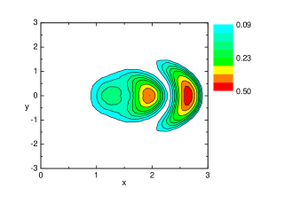
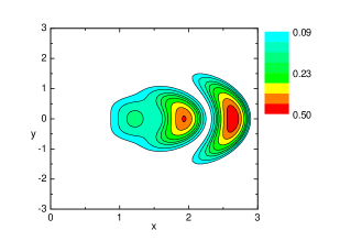
Figure 4: (color online) Probability density at $T=0.5$ in the case of a circular billiard, with ${\bf q}=(0,0)$ and ${\bf p}=(4,0)$. The upper panel shows the exact calculation and the lower one is $|\psi_{{\bf q}}(x,y)|^{2}$. Using only real trajectories we have a very good result ($|\langle\psi|\psi_{{\bf q}}\rangle|^{2}\approx 97\%$), including effects due to curvature and interference.

Figure 5: Cut of the probability densities in Fig.4 along the line $y=0$, displaying the exact (solid) and the semiclassical (dashed) results. The latter is obtained from the interference of a direct and a reflected trajectory.

We consider only the real approximation $\psi_{\bf q}$, but in this case for all final points ${\bf x}$ we should take into account the contribution of the many trajectories that reflect at the boundaries of the billiard. The actual number of such trajectories is infinite, but we consider only the two shortest ones, respectively with zero and one reflection, which give the main contributions. This gives origin to interference, as we can appreciate from Fig. 4b. The agreement with the exact result is excellent: the curvature is practically the same, as well as the height and the position of the peaks. It is important to note that there is a collision with a hard wall involved, and thus an extra phase of $\pi/2$ must be introduced in the contribution of the reflected trajectory. The overlap (51) in this case is around $97\%$. Since this approximation is already very good, we do not present the complex calculation. We show again a cut along the line $y=0$ of the probability densities, in Fig. 5. The small discrepancy could be corrected if a twice reflected trajectory was included.

IV.4 Tunnelling system

Finally we consider a system in which the tunnel effect plays an important role. We take a potential of the type

$$V(x,y)=V_{0}\exp\{-\frac{(r^{2}-r_{0}^{2})^{2}}{\sigma^{2}}\},$$ (53)

with $r^{2}=x^{2}+y^{2}$, which describes a circular ridge of radius $r_{0}$ in the plane, centered around the origin. When an incident wave packet with energy less than $V_{0}$ is scattered by this potential, there is a probability that the particle will tunnel into the ridge. In Fig. 6a we see the exact calculation at $T=2.5$, for a potential with $V_{0}=10$, $r_{0}=5$, $\sigma=10$ and an initial wave packet with ${\bf q}=(-10,0)$ and ${\bf p}=(4,0)$. The total probability of being located inside the ridge is around $10\%$ in this case.

A semiclassical calculation for tunnelling though a square barrier involving complex trajectories was presented in xavier , where only the coherent state representation $\langle z^{\prime}|e^{-iHT/\hbar}|z\rangle$ was considered. In the present case the classical motion must be solved numerically and the presence of turning points leads to the appearance of caustics. Nevertheless, provided the probability amplitude is not large in the vicinity of the caustics, the real trajectory approximation $|\psi_{{\bf q}}(x,y)|^{2}$ is able to give an accurate result, as we can see in Fig. 6b (the overlap between the transmitted wave function in the exact and semiclassical calculations is around $94\%$). This is easy to understand if we remember that for each value of the pair $(x,y)$ we need a different initial momentum ${\bf p}_{i}$ and, even though a classical particle with the average momentum ${\bf p}$ would be reflected by the potential, there will be values of ${\bf p}_{i}$ for which transmission is possible. The other real trajectory approximation $|\psi_{{\bf p}}(x,y)|^{2}$, on the other hand, works poorly in this case, because it involves variation only on the initial position and this does not affect the energy of the trajectories.

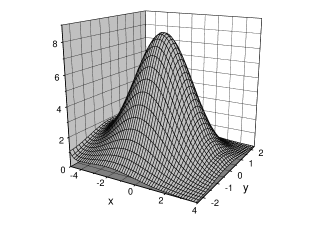
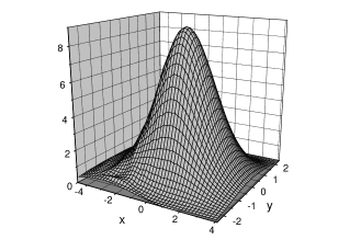
Figure 6: Probability density at $T=2.5$ for the ridge potential, with ${\bf q}=(-10,0)$ and ${\bf p}=(4,0)$. The upper panel shows the exact calculation and the lower one is $|\psi_{{\bf q}}(x,y)|^{2}$ (times $10^{2}$). Using only real trajectories it is possible to accurately reproduce tunnelling effects ($|\langle\psi|\psi_{{\bf q}}\rangle|^{2}\approx 94\%$).

The full complex semiclassical calculation would give even better results than Fig. 6b, but this requires extending the potential to the complex plane. This extension involves trigonometric functions that make the numerical evolution very demanding. It is clear that the simplicity of the trajectories involved in the calculation of $|\psi_{{\bf q}}(x,y)|^{2}$ is of great practical advantage.

V Conclusion

We have generalized the semiclassical approximation for the propagation of wave packets based on complex trajectories derived in huber ; aguiar to multidimensional systems. Several further approximations based on real trajectories were also derived from this basic formula, in particular Heller’s Thawed Gaussian Approximation (TGA). Apart from the TGA, all other formulas are not Initial Value Representations and are able to accurately reproduce non-Gaussian wave functions and also quantum interference when more than one family of trajectories is present.

These theoretical results were tested in very distinct particular cases, starting with scattering by an attractive potential, where the classical trajectories must be computed numerically. For positive energies this potential has no turning points and thus no caustics. The complex and real approximations give indistinguishable results that are very close to the exact calculation. The second case was a bound nonlinear system, where a large number of contributing classical trajectories exist. Using only the main family we obtained a very good result with the complex approximation. In this case the real trajectories approximations are not practical because of the many caustics involved. We also studied the motion inside a circular billiard, taking into account two real trajectories for $\psi_{\bf q}({\bf x},T)$, which displayed effects of curvature and interference. Finally, we considered the tunnel effect and showed that again $\psi_{\bf q}({\bf x},T)$ is able to accurately reproduce the quantum result.

All cases studied in this paper are integrable and have circular symmetry, which clearly introduces simplifications. We have also considered relatively short propagation times. For long times the number of trajectories in bound systems increases and caustics proliferate, making a practical application of the formulas more difficult. If it is possible to overcome this problem, the study of chaotic systems would naturally be the next step.

*

Appendix A

Consider a classical trajectory, satisfying Hamilton’s equation

$$\frac{d}{dt}\begin{pmatrix}{\bf x}\\ {\bf p}\end{pmatrix}=J\nabla H,$$ (54)

where $J$ is the usual symplectic matrix and $\nabla$ is the $2d$-dimensional gradient. A variation around this trajectory satisfies

$$\frac{d}{dt}\begin{pmatrix}\delta{\bf x}\\ \delta{\bf p}\end{pmatrix}=J\begin{pmatrix}H_{{\bf x}{\bf x}}&H_{{\bf x}{\bf p}}\\ H_{{\bf p}{\bf x}}&H_{{\bf p}{\bf p}}\end{pmatrix}\begin{pmatrix}\delta{\bf x}\\ \delta{\bf p}\end{pmatrix},$$ (55)

where the second derivatives of $H$ are computed at the reference trajectory. Multiplying both sides on the left by a matrix containing the inverse quantum uncertainties, $B$ and $C$, and inserting an identity in the r.h.s. we can rewrite (55) as

$$\frac{d}{dt}\begin{pmatrix}\delta\tilde{{\bf x}}\\ \delta\tilde{{\bf p}}\end{pmatrix}=\begin{pmatrix}B^{-1}H_{{\bf p}{\bf x}}B&B^{-1}H_{{\bf p}{\bf p}}C\\ -C^{-1}H_{{\bf x}{\bf x}}B&-C^{-1}H_{{\bf x}{\bf p}}C\end{pmatrix}\begin{pmatrix}\delta\tilde{{\bf x}}\\ \delta\tilde{{\bf p}}\end{pmatrix},$$ (56)

where $\tilde{{\bf x}}=B^{-1}{\bf x}$ and $\tilde{{\bf p}}=C^{-1}{\bf p}$.

Now consider a trajectory that starts from ${\bf x}^{\prime}$ with momentum ${\bf p}^{\prime}$ and arrives at ${\bf x}$ with momentum ${\bf p}$ (not related with the initial coherent state label), and suppose we make small displacements in its initial and final coordinates. This induces variations in the initial and final momenta according to

$$\left(\begin{array}[]{c}\delta{\bf p}\\ \delta{\bf p}^{\prime}\end{array}\right)=\begin{pmatrix}S_{{\bf x}{\bf x}}&S_{{\bf x}{\bf x}^{\prime}}\\ -S_{{\bf x}^{\prime}{\bf x}}&-S_{{\bf x}^{\prime}{\bf x}^{\prime}}\ \end{pmatrix}\left(\begin{array}[]{c}\delta{\bf x}\\ \delta{\bf x}^{\prime}\end{array}\right).$$ (57)

On the other hand, the tangent matrix is defined to be the linear application that relates the initial and final displacements,

$$\begin{pmatrix}\delta\tilde{{\bf x}}\\ \delta\tilde{{\bf p}}\end{pmatrix}=\begin{pmatrix}M_{{\bf x}{\bf x}}&M_{{\bf x}{\bf p}}\\ M_{{\bf p}{\bf x}}&M_{{\bf p}{\bf p}}\end{pmatrix}\begin{pmatrix}\delta\tilde{{\bf x}}^{\prime}\\ \delta\tilde{{\bf p}}^{\prime}\end{pmatrix},$$ (58)

where we have included explicitly the quantum uncertainties for convenience. Inverting equation (57) it is possible to show that

$$|-S_{{\bf x}^{\prime}{\bf x}}^{-1}|=\frac{|B|}{|C|}|M_{{\bf x}{\bf p}}|=\frac{|B|^{2}}{\hbar^{d}}|M_{{\bf x}{\bf p}}|,$$ (59)

which we have used in equation (6). It is also possible to show that $S_{{\bf x}^{\prime}{\bf x}^{\prime}}=CM_{{\bf x}{\bf p}}^{-1}M_{{\bf x}{\bf x}}B^{-1}$ and therefore

$$\Phi_{{\bf x}^{\prime}{\bf x}^{\prime}}=B^{-1}(iM_{{\bf x}{\bf p}}^{-1}M_{{\bf x}{\bf x}}-1)B^{-1},$$ (60)

where we have used $C/\hbar=B^{-1}$. This leads to

$$|\Phi_{{\bf x}^{\prime}{\bf x}^{\prime}}|=\frac{i^{d}}{|B|^{2}}\frac{|M_{{\bf x}{\bf x}}+iM_{{\bf x}{\bf p}}|}{|M_{{\bf x}{\bf p}}|},$$ (61)

as stated in equation (12). The inverse of $\Phi_{{\bf x}^{\prime}{\bf x}^{\prime}}$, used in (46), can also be expressed in terms of the tangent matrix:

$$\Phi_{{\bf x}^{\prime}{\bf x}^{\prime}}^{-1}=-iB(M_{{\bf x}{\bf x}}+iM_{{\bf x}{\bf p}})^{-1}M_{{\bf x}{\bf p}}B.$$ (62)

If we now take the time derivative of equation (58), and compare the result with (56) we conclude that

$$\frac{dM}{dt}=\begin{pmatrix}B^{-1}H_{{\bf p}{\bf x}}B&B^{-1}H_{{\bf p}{\bf p}}C\\ -C^{-1}H_{{\bf x}{\bf x}}B&-C^{-1}H_{{\bf x}{\bf p}}C\end{pmatrix}M.$$ (63)

This is the dynamical equation for the tangent matrix, which may be simplified for the large number of cases in which $H_{{\bf x}{\bf p}}=H_{{\bf p}{\bf x}}=0$ and $H_{{\bf p}{\bf p}}$ is the inverse of the mass. In practical applications these may be solved together with the equations of motion, making it possible to follow the phase of the prefactor in (13).

References

- (1) J.R. Klauder, in Path Integrals (G.J. Papadopoulos and J.T. Devreese, Eds.), Plenum, New York, 1978, p.5; Phys. Rev. D 19, 2349 (1979); Phys. Rev. Lett. 56, 897 (1986); in Random Media (G. Papanicolau, Ed.), Springer-Verlag, New York, 1987, p.163.
- (2) Y. Weissman, J. Chem. Phys. 76, 4067 (1982); J. Phys. A 16, 2693 (1983).
- (3) S. Adachi, Ann. Phys. (N.Y.) 195, 45 (1989).
- (4) A.D. Ribeiro, M.A.M. de Aguiar and M. Baranger, Phys. Rev. E 69, 66204 (2004).
- (5) A.L. Xavier Jr and M.A.M. de Aguiar, Phys. Rev. A 54, 1808 (1996); Ann. Phys. (N.Y.) 252, 458 (1996);
- (6) A.L. Xavier Jr and M.A.M. de Aguiar, Phys. Rev. Lett. 79, 3323 (1997).
- (7) F. Parisio and M.A.M. de Aguiar, Phys. Rev. A 68, 062112 (2003).
- (8) T. Van Voorhis and E.J. Heller, Phys. Rev. A 66, 050501 (2002); J. Chem. Phys. 119, 12153 (2003).
- (9) A. Rubin and J.R. Klauder, Ann. Phys. (N.Y.) 241, 212 (1995).
- (10) M. Baranger et al, J. Phys. A 34, 7227 (2001).
- (11) D. Huber and E.J. Heller, J. Chem. Phys. 87, 5302 (1987); D. Huber, E.J. Heller and R. Littlejohn, ibid 89, 2003 (1988).
- (12) M.A.M. de Aguiar et al, J. Phys. A 38, 4645 (2005).
- (13) M. Boiron and M. Lombardi, J. Chem. Phys. 108, 3431 (1998).
- (14) W.H. Miller, J. Phys. Chem. A 105, 2942 (2001); M. Thoss and H. Wang, Ann. Rev. Phys. Chem. 55, 299 (2004); K.G. Kay, ibid 56, 255 (2005).
- (15) J.H. Vleck, Proc. Natl. Acad. Sci. U.S.A. 14, 178 (1928).
- (16) M. Gutzwiller, Chaos in Classical and Quantum Mechanics (Springer, New York, 1990).
- (17) F. Parisio and M.A.M. de Aguiar, to appear.
- (18) G.G. Stokes, Trans. Cambridge Philos. Soc. 10, 106 (1864); 11, 412 (1871).
- (19) R.B. Dingle, Asymptotic Expansions: Their Derivation and Interpretation (Academic Press: London, 1973).
- (20) M.V. Berry, Proc. R. Soc. London A 422, 7 (1989).
- (21) A. Shudo and K.S. Ikeda, Phys. Rev. Lett. 76, 4151 (1996).
- (22) E.J. Heller, J. Chem. Phys. 94, 2723 (1991).
- (23) E.J. Heller in Chaos and Quantum Physics, edited by M.J. Giannoni, A. Voros and J. Zinn-Justin, Les Houches Session LII, 1989 (Elsevier, Amsterdam, 1991).
- (24) S. Tomsovic and E.J. Heller, Phys. Rev. Lett. 67, 664 (1991); M.A. Sepúlveda, S. Tomsovic and E.J. Heller, ibid 69, 402 (1992).
- (25) S. Tomsovic and E.J. Heller, Phys. Rev. E 47, 282 (1993).
- (26) M. Novaes, quant-ph/0507124.
- (27) E.J. Heller, J. Chem. Phys. 62, 1544 (1975).
- (28) G.A. Fiete and E.J. Heller, Phys. Rev. A 68, 022112 (2003).
- (29) E.J. Heller, Phys. Rev. Lett. 53, 1515 (1984).
- (30) R.A. Jalabert and H.M. Pastawski, Phys. Rev. Lett. 86, 2490 (2001).
- (31) C. Petitjean and P. Jacquod, Phys. Rev. E 71, 036223 (2005).
- (32) J. Vaníek and E.J. Heller, Phys. Rev. E 68, 056208 (2003).