Chaotic Tunneling in a Laser Field

Abstract

We study the driven tunneling of a one-dimensional charged particle confined to a rectangular double-well. The numerical simulation of the Schrödinger equation based on the Cranck-Nicholson finite-difference scheme, shows that the modulation of the amplitude of the external field may result in the parametric resonance. The latter is accompanied by the breakdown of the quasi-periodic motion characteristic of the usual driven tunneling, and the emergence of an irregular dynamics. We describe the above breakdown with the occupation probability for the ground state of the unperturbed system, and make the visualization of the irregular dynamics with the help of Shaw-Takens’ reconstruction of the state-space. Both approaches agree as to the values of the resonant frequency for the parametric excitation. Our results indicate that the shape of the laser pulse could be essential for generating chaotic tunneling.

1. Driven transitions in a double well are instrumental for studying the tunneling in various fields of physics and chemistry, mont , milena . Considerable attention has been drawn to the tunneling dynamics in the presence of a driving force with a time dependent amplitude. In his seminal paper, holthaus , M. Holthaus showed that shaping the driving force may be instrumental in controlling the tunneling in a bistable potential. In particular, it was shown, holthaus , that choosing an appropriate envelope for laser pulse, one may perform the population transfer on time scales much shorter than the base tunneling time. This situation is intimately related to the problem of quantum chaos, which is generally approached within the framework of the quasi-classical approximation and Gutzwiller’s theory. In fact, classical chaotic systems are often used as a clue to the quantum ones. In contrast, it would be very interesting to look at the quantum chaos the other way round and consider systems which need studying without approximations that could have bearing upon classical mechanics, for example, particles confined to potentials of a size comparable with the de Broglie wave length. This has also an additional interest owing to the fact that calculations within the framework of semiclassical theory should depart from the quantum ones on the time scale of $\hbar/\Delta E$, $\Delta E$ being the typical spacing between energy levels. Therefore, the Schrödinger equation describing the problem needs numerical studying.

This letter aims at the theoretical description of the tunneling transitions for a charged particle in a one-dimensional rectangular double-well potential $U(x)$ and an external periodic field $V(t)$ that mimics electro-magnetic irradiation. The Hamiltonian of the system in dimensionless units is given by the equation

$$H=\frac{1}{2}\,\hat{p}^{2}+U(x)+V(t)$$

in which the potential $U$ reads

$$U=\left\{\begin{array}[]{rl}-U_{1},&a\leq x\leq b\\ -U_{2},&c\leq x\leq d\\ 0,&\mbox{otherwise}\end{array}\right.$$ (1)

i.e. the unsymmetrical double well comprising the two shafts of different depths $U_{1},U_{2}$, see FIG.1. The shape of $U$ is chosen in such a way that the values of the wave functions, $\psi_{0}(x,t)=<x|0>,\quad\psi_{1}(x,t)=<x|1>$, of the ground and the first excited state, are very small outside the right and the left shafts of the well, respectfully, see FIG.1. Consequently, the particle’s transitions $|0>\rightleftharpoons|1>$ can be visualized as the tunneling ones. The field frequency $\Omega$ verifies the constraint of resonance, which in dimensionless units reads $\Omega=E_{1}-E_{0}$, where $E_{0},\,E_{1}$ are the energies of the ground and the first excited states. The external field $V(t)$ has the form

$$V(t)=-A\,\sin(\Omega t)\,\hat{p},\quad\hat{p}=-i\partial_{x}$$

where $\hat{p}$ is the operator of momentum, corresponding to an electro-magnetic wave described by the vector potential $A_{x}=A_{z}=0,A_{y}=A\sin\Omega(t-x/c)$, the scalar potential $\phi$ being equal to zero, scully . In what follows we neglect the dependence of $A$ on $x$ since the wave length is assumed to be much larger than the well’s size.

We are looking for regimes in which the regular tunneling breaks down and becomes chaotic. The main instrument employed for this end, is the Shaw-Takens (ST) method, shtk , for reconstructing the state-space of a system from a stream of data, obtained with the numerical integration of the Schrödinger equation, by embedding it in a phase space of enough dimension ${\cal D}$, in our case ${\cal D}=3$. The important thing is that one may monitor the dynamics of driven tunneling, by using the occupation probability $N_{0}$ of the ground state of the unperturbed system

$$N_{0}=|<0|\psi>|^{2},$$

where $|0>$ and $|\psi>$ are the ground vector, and the state vector of the system at the moment of time $t$, respectively. To obtain the visualization we shall form a time series that comprises the values of $N_{0}$ at moments of time $n\tau,\quad n=0,1,2,\ldots,$; $\tau$ being the lag-time, so that $N_{0k}=N_{0}(k\tau),\,k=1,2,3,\ldots$ . Then the series of vectors $Y_{k}=(N_{0k},N_{0k+1},N_{0k+2}),k=0,1,2,3,\ldots$, serves a 3d-visualization of the state-space for the given problem. In particular, we can observe the transition from the regular motion characteristic of the unperturbed resonant motion to the irregular one generated by a parametric excitation given by Eq.(2) below, see FIG.2.

Figure 1: Rectangular one-dimensional double-well potential. Lines ”0” and ”1” indicate the moduli of the wave functions $|\psi_{0}(x,t)|$ and $|\psi_{1}(x,t)|$ of the ground and the first excited states. In the chosen configuration $D=0.876$ is the distance between the wells; $L_{0}=2.337,L_{1}=2.045$ are the widths, and $U_{0}=13.82,U_{1}=11.91$ are the depths of the shafts in dimensionless units.

2. The parametric excitation of the system is generated by the modulation of the amplitude $A$ of the vector potential

$$A=A_{0}[1-\epsilon\sin(\omega t)]$$ (2)

The approximate expression for the frequency of the parametric resonance caused by (2) can be obtained by employing the rotating wave approximation, scully after some analytical calculations. It reads

$$\omega_{prm}=A\kappa,\quad\kappa=|<0|\hat{p}|1>|$$ (3)

In fact, the actual resonant frequency $\omega_{prm}$ differs from that given above and its calculation requires some numerical work.

3. The visualization with the help of the ST-method gives a torus in 3d-space, fairly well drawn, changes in the lag-time resulting only in continuous deformations of the picture, and no sudden modifications observed, see FIG.2. In contrast, in case the parametric excitation at a frequency close to the value given by (3), being present, the choice of the lag-time is very important for obtaining a meaningful visualization. The break down of the quasi-periodic motion by the resonant parametric excitation is shown in FIG.2. It is to be noted that the visualization depends on a number of premises, and first of all the value of the lag-time $\tau$ and the dimension $d$ of the visualization window. The wise choice of $\tau$ is dictated by characteristic times of the motion under the investigation, so that for certain values of $\tau$ the visualization picture is coherent enough whereas for others it is not meaningful. Therefore, using the ST-method one has to compare pictures obtained for different values of the lag-time.

4. We may look at our problem the other way round. Consider sets of the system’s states ${\cal F}_{kk+1},\,k=1,2,\ldots,{\cal N}$, where ${\cal N}$ is large enough, given by constraints

$$\Delta_{k}\leq N_{0}\leq\Delta_{k+1},$$ (4)

where $\Delta_{k}$ are intervals dividing segment $0\leq N_{0}\leq 1$ in ${\cal N}$ equal parts. Take a period of time $T$, sufficiently large, and consider times $\tau_{k}$ spent by the system in the sets of states ${\cal F}_{kk+1}$, that is where (4) is verified. We shall define the visiting frequencies as

$$\nu_{kk+1}=\frac{\tau_{k}}{T}$$

One may cast the $\nu_{kk+1}$ in the form of the probability density, $\xi(N_{0})$, for the distribution of $N_{0}$, by assuming that all the intervals $\Delta_{k+1}-\Delta_{k}$ be of equal size $\Delta$, and defining

$$\xi(N_{0})=\frac{\nu_{kk+1}}{\Delta}$$

On considering the limit of $\xi$ as ${\cal N}\to\infty$, we shall get the probability density $\xi(N_{0})$, see FIG.3.

To put it in a quantitative analytical form, we may consider the characteristic function $\chi_{ab}(x)=1,\mbox{if}\quad a\leq x\leq b$ and $0$ otherwise, and introduce the quantity

$$\nu_{\phi}(a,b)=\lim_{T\rightarrow\infty}\left\{\frac{1}{T}\int_{-T/2}^{+T/2}\,\chi_{ab}(N_{0})\,dt\right\},$$ (5)

so that $\nu_{ab}$ can be considered as the frequency of visiting a region of states determined by constraint $a\leq N_{\phi}\leq b$.

The important point is that the limit indicated in the above equation does exist in the context of the problem under investigation. To see the fact we shall employ the normalization of wave functions in a finite box, that is, our system being confined to a rectangular potential of infinite depth of a size much larger than the double well’s size. Then the system has the discrete spectrum of eigenvalues, and the characteristic function $\chi_{ab}(N_{0})$ can be expanded in Fourier series, the time averaging in the above equation results in cancelling out terms oscillating in time, so that the limit exists. The use of the finite box normalization is also important for managing the numerical simulation. It is alleged to be known, the finite integration mesh, or basis, results in reflection of the wave packet that distorts the time evolution of the packet. By imposing the finite box normalization we use the physical framework that appears to be compatible with the tunneling dynamics in the double well of a size much smaller than the box and enables us to overcome the numerical artifacts.

It is worth noting that the construction of visiting frequencies is analogous to that of the dwell time which is aimed at studying the localization of wave packets and defined by the equation, buttiker , nuss ,

$$\tau_{D}(a,b)=\int^{+\infty}_{-\infty}\,dt\,\int^{b}_{a}\,|\psi(x,t)|^{2}\,dx$$

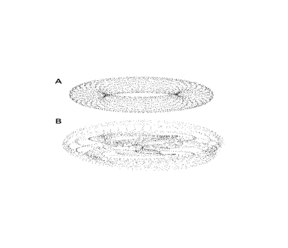
Figure 2: Visualization of the state space. A no parametric excitation. B parametric excitation: $A_{0}=0.3;\epsilon=0.1;\omega=0.01755$. The lag-time $330$, in both cases.

The probability density $\xi$ indicates that at the resonant frequency $\omega_{prm}$ the character of the system’s motion undergoes a drastic change, see FIG.3. At this point it should be noted that the frequency of the parametric resonance $\omega_{prm}$ which can be found by comparing the sizes of the peaks in FIG.3 for different values of $\omega$ in equation (2), differs by approximately $5\%$ from the value given by the rotation wave approximation (3). The resonant value corresponds to the most pronounced breakdown of the twin peaks, which correspond to the ground and the first excited state of the free system.

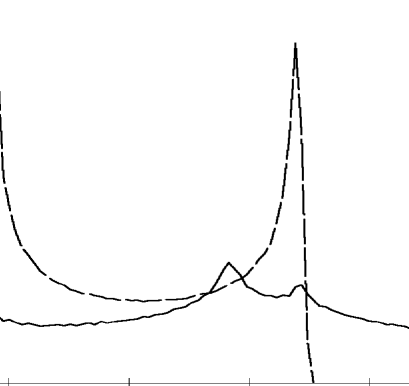
Figure 3: Probability density $\xi$ for the distribution of $N_{0}$ with $A_{0}=0.3$; 6 six bound states (levels confined to the well). Dashed line - no parametric excitation. Solid line - parametric excitation with $\epsilon=0.1$., parametric frequency $\omega=0.01755$ close to the resonant one, $\omega_{prm}$

5. Concluding we should like to note that, as follows from Eq.(2) for the amplitude of the driving force, the pulse $V$ has a triplet structure determined by the main contribution at frequency $\Omega=E_{1}-E_{0}$ and two satellites at $\Omega\pm\omega_{prm}$, of less amplitude, owing to the equation for $A(t)$ given by (2)

$$A(t) = A_{0}\kappa\,\,\sin\Omega t-\frac{1}{2}A_{0}\kappa\,\epsilon\,\cos[(\Omega-\omega_{prm})t]$$

$$+ \frac{1}{2}A_{0}\kappa\,\epsilon\,\cos[(\Omega+\omega_{prm})t]$$

The triplet structure could generally have an important bearing on the tunneling in the double-well potential. In fact, if a monochromatic pulse at resonant frequency $\Omega=E_{1}-E_{0}$ is employed, there is no parametric excitation and the dynamics of the occupation probability has the usual form. In contrast, a poor quality non-monochromatic pulse may contain the triplet $\Omega\pm\omega_{prm}$ so that the deformation of the tunneling dynamics and the emergence of the chaotic motion become possible. It is worth noting that the amplitude of the driving force, $A_{0}$, can be small so that the frequency shift determined by $\omega_{prm}$ be tiny.

Acknowledgment
This work was supported by the grants NS - 1988.2003.1, and RFFI 01-01-00583, 03-02-16173, 04-04-49645.

References

- (1) D.T.Monteiro, S.M.Owen, and D.S.Saraga, Manifestations of chaos in atoms, molecules and quantum wells, Phil.Trans.R.Soc.Lond. A 357, 1359 (1999).
- (2) M.Grifoni and P.Hänggi, Driven Quantum Tunneling, Phys.Reports 304, 229 (1998).
- (3) M.Holthaus, Phys.Rev.Lett. 69, 1596 (1992).
- (4) N.H.Packard, J.P.Crutchfield, J.D.Farmer, and R.S.Shaw, Phys.Rev.Lett. 47, 712 (1980).
- (5) M.O.Scully and M.S.Zubairy, Quantum Optics, Ch.5, Cambridge University Press, Cambridge (1999).
- (6) M.Büttiker, Phys.Rev. B27, 6178 (1983).
- (7) H.M.Nussenzveig, Phys.Rev. A62, 042107 (2000).