Hidden measurements, hidden variables and the volume representation of transition probabilities

We construct, for any finite dimension $n$, a new hidden measurement model for quantum mechanics based on representing quantum transition probabilities by the volume of regions in projective Hilbert space. For $n=2$ our model is equivalent to the Aerts sphere model and serves as a generalization of it for dimensions $n\geq 3$. We also show how to construct a hidden variables scheme based on hidden measurements and we discuss how joint distributions arise in our hidden variables scheme and their relationship with the results of Fine [15].

Key words: hidden measurements, hidden variables, classical representations of quantum probability

1 INTRODUCTION

Hidden measurements were introduced by Aerts [2] to show that it is possible to understand quantum probabilities as arising from a lack of knowledge about the interactions between a measuring device and the system that it is measuring. In this way, quantum mechanics can be understood within classical probability theory with the peculiarities of quantum probabilities arising from a simple lack of knowledge and not some mysterious source. The hidden measurement formalism is just one of a number of approaches that try to find a classical representation for probability structures in quantum mechanics. For example, stochastic extensions of the Schrödinger equation have been proposed to account for the collapse of the wave function [1, 16] and hence the appearance of quantum probabilities. It has also been observed that quantum like behavior can arise within classical systems [20, 14, 2, 4, 17, 18]. The fact that it is possible to find classical representations for the probability structures in quantum mechanics and that quantum like behavior arises in non-quantum systems hints that eventually quantum mechanics will be understood within classical probability theory.

To describe hidden measurements, we denote by $X$ the set of possible states of a system $S$ and by $Y$ the set of possible states of the measuring device $\mathcal{M}$ used to measure $S$. Given that the system is in a state $x\in X$ and the measuring device is in the state $y\in Y$, we let $z=\mathcal{M}(x,y)$ denote the outcome of the measurement. The measurement is assumed to be deterministic so if we let $Z$ denote the collection of all possible measurement outcomes then $(x,y)\mapsto\mathcal{M}(x,y)$ defines a map from $X\times Y$ to $Z$. The fact that the result of a measurement depends on the state of the measuring device is the justification for the name “hidden measurements”.

To formalize the above discussion, we need two measure spaces $(X\times Y,\mathcal{A}(X\times Y))$ and $(Z,\mathcal{A}(Z))$. Here we are using $\mathcal{A}(X\times Y)$ and $\mathcal{A}(Z)$ to denote $\sigma$-algebras on $X\times Y$ and $Z$, respectively. A deterministic measurement is defined to be a measurable map (i.e. a random variable)

$$\mathcal{M}:X\times Y\longrightarrow Z\,.$$ (1.1)

The state of the system plus measuring device is assumed to be uncertain and characterized by a probability measure $\mu$ on $(X\times Y,\mathcal{A}(X\times Y))$. The probability of a measurement yielding an event $U\in\mathcal{A}(Z)$ is then given by

$$\text{Prob}(\mathcal{M}\in U\,|\,\mu):=\int_{\mathcal{M}^{-1}(U)}\mu\,.$$ (1.2)

From this it can be seen that the probability of a measurement obtaining a certain value is due not only to the uncertainty of the system but also to the uncertainty in the state of the measuring device which is characterized by the measure $\mu$. Even in the situation where there is no uncertainty in the state of the system there can still be uncertainty in the state of the measuring device and hence the outcome of a measurement is probabilistic. In the terminology of [5], a deterministic measurement is referred to as rule of interaction. In that paper, the special case where the measure $\mu$ in (1.2) factors as a product of measure on $X$ and $Y$ (i.e. $\mu=\mu_{X}\mu_{Y}$) is called an interactive probability model. For more discussion on the philosophical foundations of the hidden measurement formalism we refer the readers to the papers [2, 3] and references cited therein.

The hidden measurement formalism has continued to be developed by a number of authors and various hidden measurement schemes have been constructed [8, 6, 7, 4, 12, 11, 5]. The range of possible hidden measurement schemes have been classified in [9, 10] and for finite dimensional quantum systems no preferred scheme is identified. Criteria for selecting out a preferred scheme is still lacking and thus different hidden measurement schemes should be investigated so their relative merits can be compared.

The aim of this article is to introduce a new hidden measurement scheme for finite dimensional quantum systems based on the concept of representing quantum transition probabilities by the volume of regions of projective Hilbert space. Since the measure we use in constructing the hidden measurement scheme factors, our construction defines an interactive probability model. For dimension $n=2$ our scheme is isomorphic to the sphere model of Aerts [2, 14]. This can be seen through the isomorphism $\mathbb{P}\mathcal{H}\cong S^{2}$. For dimensions $n\geq 3$ our approach offers a significant improvement over previous schemes in that it is geometrical in origin and is formulated on projective Hilbert space (i.e. we take $X=Y=\mathbb{P}\mathcal{H}$ for some Hilbert space $\mathbb{P}\mathcal{H}$ ) which is the natural state space of quantum mechanics. This allows for a clear understanding of how the group of unitary transformations acts on our hidden measurement scheme.

With the exception of the $2$ and $3$ dimensional models presented in [2] and [4], previous hidden measurement models have essentially used, in the notation above, $X=\mathcal{H}$ or $S(\mathcal{H})$ and for $Y$ a simplex sitting in $\mathbb{R}^{n}$. The choice of the simplex for $Y$ arose from the observation that given a quantum state $\psi$ and an orthonormal basis $\{\psi_{1},\ldots,\psi_{n}\}$, the transition probabilities $p_{\psi_{k}}(\psi):=|\langle\psi|\psi_{k}\rangle|^{2}$ regarded as a vector $(p_{\psi_{1}}(\psi),\ldots,p_{\psi_{n}}(\psi))$ must lie in the simplex $\{(x_{1},\ldots,x_{n})\,|\,x_{i}\geq 0\;\text{and}\;\sum_{i}x_{i}=1\}$. The hidden measurement scheme is then implemented by partitioning the simplex into $n$ regions with volume equal to the transition probabilities $p_{\psi_{k}}(\psi)$. The limitations of the scheme is that for each commuting set of observables a new simplex must be introduced and a priori it is unclear how the different measurement systems are related. We note that in [13] it is shown that by fixing one hidden measurement scheme for one set of commuting observables that it is possible to use a group translation procedure to induce hidden measurement schemes for the other commuting sets of observables in a manner that is consistent with quantum mechanics. However, due to the abstract method of enforcing the action of the unitary group it is difficult to get a global picture of the measurement scheme and the relations between different observables. In contrast our method supplies a hidden measurement scheme for each set of commuting observables and at the same time provides a natural action of the unitary group on the schemes and shows that the entire collection is compatible with quantum mechanics. The action of the unitary group is natural and easy to understand.

We also show how to construct a hidden variables scheme based on hidden measurements. Here we are taking the term hidden variables to mean representing quantum observables and quantum states as random variables and probability distributions, respectively, on a fixed space. Due to the nature of the measurement depending on the state of the measuring device, the type of hidden variables that we construct are contextual. A general discussion of this point can be found in [13] where it is shown that for any hidden measurement system it is possible to introduce a (non-unique) contextual hidden variables theory. Finally, we discuss how joint distributions for commuting observables arise in our hidden variables scheme and their relationship with the results of Fine [15].

2 PROJECTIVE HILBERT SPACE

In this section we review some basic results about projective Hilbert space. We use the book [19] as our standard reference. Let $(\mathcal{H},\langle\cdot|\cdot\rangle)$ be a complex Hilbert space where the inner product $\langle\cdot|\cdot\rangle$ is taken to be linear in the second variable. Define

$$\mathcal{H}^{\times}:=\mathcal{H}\setminus\{0\}\quad\text{and}\quad\mathbb{C}^{\times}:=\mathbb{C}\setminus\{0\}.$$ (2.1)

On $\mathcal{H}^{\times}$ we can define an equivalence relation $\sim$ by $\psi\sim\phi$ if and only if there exists a $\lambda\in\mathbb{C}^{\times}$ such that $\psi=\lambda\phi$. Letting $[\psi]$ denote the equivalence class for $\psi\in\mathcal{H}^{\times}$, we have

$$[\psi]:=\{\,\lambda\psi\,|\,\lambda\in\mathbb{C}^{\times}\,\}\;.$$ (2.2)

Projective Hilbert space $\mathbb{P}\mathcal{H}$ is then defined as

$$\mathbb{P}\mathcal{H}:=\mathcal{H}^{\times}/\sim=\{\,[\psi]\,|\,\psi\in\mathcal{H}^{\times}\,\}\,.$$ (2.3)

It is well known that $\mathbb{P}\mathcal{H}$ carries a Hilbert manifold structure for which the canonical projection $\pi:\mathcal{H}^{\times}\rightarrow\mathbb{P}\mathcal{H}\;;\;\psi\mapsto[\psi]$ is a $C^{\infty}$ submersion. As a consequence for any $q\in\mathbb{P}\mathcal{H}$ and $v_{q}\in\text{T}_{q}\mathbb{P}\mathcal{H}$ there exists a $\psi\in\mathcal{H}^{\times}$ and $\phi\in\mathcal{H}$ such that $q=[\psi]$ and $v_{q}=\text{T}_{\psi}\pi\cdot\phi$. Here we are using $T_{q}\mathbb{P}\mathcal{H}$ to denote the tangent space of $\mathbb{P}\mathcal{H}$ at $q\in\mathbb{P}\mathcal{H}$ and $T_{\psi}\pi:\text{T}_{\psi}\mathcal{H}^{\times}\cong\mathcal{H}\rightarrow T_{[\psi]}\mathbb{P}\mathcal{H}$ to denote the tangent map of the mapping $\pi:\mathcal{H}^{\times}\rightarrow\mathbb{P}\mathcal{H}$. The above representations for points and tangent vectors on $\mathbb{P}\mathcal{H}$ can be used to define a complex structure $\mathbb{J}$ and a strongly non-degenerate symplectic form $\omega$ on $\mathbb{P}\mathcal{H}$ via the formulas

$$\mathbb{J}(\text{T}_{{\psi}}\pi\cdot\phi):=\text{T}_{\psi}\pi\cdot i\phi$$ (2.4)

and

$$\omega_{[\psi]}(\text{T}_{\psi}\pi\cdot\phi_{1},\text{T}_{\psi}\pi\cdot\phi_{2}):=2\hbar\|\psi\|^{-4}\text{Im}\left(\langle\phi_{1}|\phi_{2}\rangle\|\psi\|^{2}-\langle\phi_{1}|\psi\rangle\langle\psi|\phi_{2}\rangle\right)$$ (2.5)

for every $\psi\in\mathcal{H}^{\times}$ and $\phi,\phi_{1},\phi_{2}\in\mathcal{H}$. Recall that a symplectic form is a non-degenerate closed two form. It should be noted that $g(v,w)=\omega(v,\mathbb{J}w)$ defines a Riemannian metric on $\mathbb{P}\mathcal{H}$ and hence establishes that $\mathbb{P}\mathcal{H}$ is a Kähler manifold.

Given a function $f\in C^{\infty}(\mathbb{P}\mathcal{H})$, the non-degeneracy of the symplectic form $\omega$ implies that the following equation

$$\omega(X_{f},Y)=\text{d}f(Y)\quad\text{for all vector fields $Y$ on $\mathbb{P}\mathcal{H}$},$$ (2.6)

uniquely defines a vector field $X_{f}$. The Poisson bracket $\{\cdot,\cdot\}$ is then defined via

$$\{f,g\}:=\omega(X_{f},X_{f})\quad\forall\;f,g\in C^{\infty}(\mathbb{P}\mathcal{H})\;.$$ (2.7)

Let $\mathcal{L}(\mathcal{H})$ denote the set of bounded linear operators on $\mathcal{H}$. Then the unitary group $\text{U}(\mathcal{H})$ is defined by

$$\text{U}(\mathcal{H}):=\{U\in\mathcal{L}(\mathcal{H})\,|\,\langle U\psi|U\phi\rangle=\langle\psi|\phi\rangle\quad\forall\psi,\phi\in\mathcal{H}\,\}\;.$$ (2.8)

Its Lie algebra $\mathfrak{u}(\mathcal{H})$ is the set of skew-adjoint operators, i.e.

$$\mathfrak{u}(\mathcal{H}):=\{A\in\mathcal{L}(\mathcal{H})\,|\,A^{\dagger}=-A\,\}\,.$$ (2.9)

Here we are using $\dagger$ to denote the adjoint of an operator. The following map

$$\rho\;:\;\text{U}(\mathcal{H})\times\mathbb{P}\mathcal{H}\rightarrow\mathbb{P}\mathcal{H}\;:\;(U,[\psi])\rightarrow[U\psi]$$ (2.10)

defines an action of $\text{U}(\mathcal{H})$ on $\mathbb{P}\mathcal{H}$ by symplectomorphism (i.e. $\rho_{U}^{*}\omega=\omega$ for all $U\in\text{U}(\mathcal{H})$). There also exists an equivariant momentum mapping $\text{J}\,:\,\mathbb{P}\mathcal{H}\longrightarrow\mathfrak{u}(\mathcal{H})^{*}$ for this action defined by

$$\langle\text{J}([\psi]),A\rangle:=i\hbar\frac{\langle\psi|A\psi\rangle}{\|\psi\|^{2}}\quad\forall\;\psi\in\mathcal{H},\,A\in\mathfrak{u}(\mathcal{H})\,,$$ (2.11)

where $\langle\cdot,\cdot\rangle$ denotes the canonical pairing between $\mathfrak{u}(\mathcal{H})^{*}$ and $\mathfrak{u}(\mathcal{H})$. Letting $\mathcal{C}^{\infty}(\mathbb{P}\mathcal{H})$ denote the set of smooth functions on $\mathbb{P}\mathcal{H}$, the momentum map can be viewed as a map $\text{J}\,:\,\mathfrak{u}(\mathcal{H})\longrightarrow\mathcal{C}^{\infty}(\mathbb{P}\mathcal{H})$ by defining

$$\text{J}(A)(x):=\langle\text{J}(x),A\rangle\quad\forall\;x\in\mathbb{P}\mathcal{H}\;.$$ (2.12)

Recall that the defining property of a momentum map is that

$$\omega(\underline{A},Y)=\text{d}\text{J}(A)(Y)$$ (2.13)

holds for all vector fields $Y$ on $\mathbb{P}\mathcal{H}$ and $A\in\mathfrak{u}(\mathcal{H})$ where $\underline{A}$ is the vector field on $\mathbb{P}\mathcal{H}$ generated by $A$, i.e.

$$\underline{A}([\psi]):=\frac{d\,}{dt}\Bigl{|}_{t=0}\rho_{\exp(tA)}([\psi])=T_{\psi}\pi\cdot A\psi,$$ (2.14)

while an equivariant momentum map satisfies the additional condition

$$\langle\text{J}\circ\rho_{U}(x),A\rangle=\langle J(x),U^{-1}AU\rangle\quad\forall\,x\in\mathbb{P}\mathcal{H},A\in\mathfrak{u}(\mathcal{H}),U\in\text{U}(\mathcal{H})\,.$$ (2.15)

It follows from the equivariance that

$$\{\text{J}(A),\text{J}(B)\}=\text{J}([A,B])\quad\forall\;A,B\in\mathfrak{u}(\mathcal{H})\,.$$ (2.16)

Let $\text{Sa}(\mathcal{H})$ denote the set of bounded self-adjoint operators on $\mathcal{H}$. For each operator $H\in\text{Sa}(\mathcal{H})$

$$\langle H\rangle:=\text{J}(-\textstyle\frac{i}{\hbar}H)\,$$ (2.17)

defines a smooth function on $\mathbb{P}\mathcal{H}$. This function is just the usual expectation of the observable $H$, i.e.

$$\langle H\rangle([\psi])=\frac{\langle\psi|H\psi\rangle}{\|\psi\|^{2}}\,.$$ (2.18)

With this notation (2.16) can be written in the more familiar form

$$\{\langle A\rangle,\langle B\rangle\}=\langle\textstyle\frac{i}{\hbar}[B,A]\rangle\;.$$ (2.19)

3 ACTION ANGLE COORDINATES ON $\mathbb{P}\mathcal{H}$

For the remainder of this article, we will assume that $\dim\mathcal{H}=N<\infty$. Let $\{\psi_{1},\ldots,\psi_{N}\}$ be an orthonormal basis for $\mathcal{H}$. Define the projection operators

$$P_{\psi_{k}}=|\psi_{k}\rangle\langle\psi_{k}|\,.$$ (3.1)

We can use the momentum map to define smooth functions $p_{\psi_{k}}$ on $\mathbb{P}\mathcal{H}$ by

$$p_{\psi}:=\langle P_{\psi_{k}}\rangle\,.$$ (3.2)

Using (2.18) we get that

$$p_{\psi}([\psi])=\frac{\langle\psi_{k}|\psi\rangle}{\|\psi\|}^{2}$$ (3.3)

which is the transition probability from the state $\psi$ to $\psi_{k}$. As the operators $P_{\psi_{k}}$ commute, formula (2.19) shows that the functions $\{p_{\psi_{1}},\ldots,p_{\psi_{N}}\}$ are in involution, i.e.

$$\{\psi_{j},\psi_{k}\}=0\quad\forall\;j,k=1,2,\ldots N\,.$$ (3.4)

It follows from $\mathord{{\mathrm{1}}\kern-2.70004pt{\mathrm{I}}}\kern 3.50006pt=\sum_{k=1}^{N}P_{\psi_{k}}$ that

$$\sum_{j=1}^{N}p_{\psi_{k}}=1\,,$$ (3.5)

which shows that at most $(N-1)$ of the functions $p_{\psi_{k}}$ can be independent. It is not hard to show that the set $\{p_{\psi_{2}},\ldots,p_{\psi_{N}}\}$ is independent. That is the set of points in $\mathbb{P}\mathcal{H}$ for which the covectors $\{dp_{\psi_{2}},\ldots,dp_{\psi_{N}}\}$ are linearly dependent has measure zero. Consequently, we can use these functions to construct action angle coordinates of $\mathbb{P}\mathcal{H}$ following the standard recipe, see [19] for details. This results in the following coordinate chart

$$\tau:T^{N-1}\times S\longrightarrow\mathbb{P}\mathcal{H}$$

$$(\theta,\mathbf{I})=((\theta_{2},\ldots,\theta_{N}),(I_{2},\ldots,I_{N}))\mapsto\Bigl{[}\bigl{(}1-\sum_{k=2}^{N}I_{k}\bigr{)}^{1/2}\psi_{1}+\sum_{j=2}^{N}e^{-i\theta_{j}}\sqrt{I_{j}}\psi_{j}\Bigr{]}$$ (3.6)

where $T^{N-1}$ is the $(N-1)$ torus and

$$S:=\Bigl{\{}\,(I_{2},\ldots,I_{N})\in\mathbb{R}^{N-1}\,|\,0<I_{j}\,\;\sum_{j=2}^{N}I_{j}<1\Bigr{\}}\,.$$ (3.7)

In this chart, the symplectic form $\omega$ is given by

$$\omega=\hbar\sum_{j=2}^{N}d\theta_{k}\wedge dI_{k}\,.$$ (3.8)

We also note that the functions $p_{\psi_{k}}$ have the coordinate representations $p_{\psi_{j}}(\theta,\mathbf{I})=I_{j}$ for $j=2,3,\ldots,N$. Using $\omega$, we can define a volume form $\nu$ on $\mathbb{P}\mathcal{H}$ by

$$\nu:=\left(\frac{-1}{2\pi\hbar}\right)^{N-1}\underset{\text{N-1 times}}{\underbrace{\omega\wedge\ldots\wedge\omega}}\;.$$ (3.9)

Locally this is given by

$$\nu=\frac{(N-1)!}{(2\pi)^{(N-1)}}\,d\theta_{2}\wedge\ldots\wedge\theta_{N}\wedge dI_{2}\wedge\ldots\wedge dI_{N}\,.$$ (3.10)

Then because the chart (3.6) covers all of $\mathbb{P}\mathcal{H}$ except for a set of measure zero, the volume of $\mathbb{P}\mathcal{H}$ is given by

$$\text{Vol}(\mathbb{P}\mathcal{H})=\frac{(N-1)!}{(2\pi)^{(N-1)}}\int_{0}^{2\pi}\ldots\int_{0}^{2\pi}d\theta_{2}\ldots d\theta_{N}\int_{S}dI_{2}\ldots dI_{N}\,.$$ (3.11)

A straightforward calculation shows that $\int_{S}dI_{2}\ldots dI_{N}=1/(N-1)!$ and hence $\text{Vol}(\mathbb{P}\mathcal{H})=1$.

4 VOLUME REPRESENTATION OF TRANSITION PROBABILITIES

Suppose $\psi,\phi\in\mathcal{H}^{\times}$. Then the transition probability from the state $\psi$ to $\phi$, or vice versa, is given by

$$T(\psi,\phi):=\frac{|\langle\psi|\phi\rangle|^{2}}{\|\psi\|^{2}\|\phi\|^{2}}\;.$$ (4.1)

As this formula is invariant under scaling of $\phi$ or $\psi$ by non-zero complex numbers, it passes to a well defined function on $\mathbb{P}\mathcal{H}\times\mathbb{P}\mathcal{H}$ given by

$$T([\psi],[\phi])=\frac{|\langle\psi|\phi\rangle|^{2}}{\|\psi\|^{2}\|\phi\|^{2}}\;\quad\forall\;\psi,\phi\in\mathcal{H}^{\times}\,.$$ (4.2)

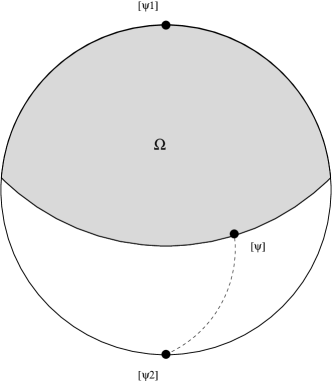
Figure 1: Volume representation of transition probabilities

It was shown in [21] that if we let $d(x,y)$ denote the geodesic distance between points $x,y\in\mathbb{P}\mathcal{H}$ then the distance $d(x,y)$ is related to the transition probability $T(x,y)$ via the formula

$$T(x,y)=\cos^{2}\Bigl{(}\frac{d(x,y)}{\sqrt{2\hbar}}\Bigr{)}\,.$$ (4.3)

This shows that there exists a representation of the transition probability in terms of the geodesic distance. The question now is, are there other representations for the transition probability in terms of geometrical objects on $\mathbb{P}\mathcal{H}$? We will show that the transition probability, at least for finite dimensional Hilbert spaces, can be related to the volume of certain regions in $\mathbb{P}\mathcal{H}$. To motivate this, we will first look at $\mathbb{P}\mathcal{H}$ where $\mathcal{H}$ is a 2 dimensional Hilbert space. Recall that $\mathbb{P}\mathcal{H}\cong S^{2}$ where $S^{2}$ is the ordinary two sphere in $\mathbb{R}^{3}$. Suppose $\{\psi_{1},\psi_{2}\}$ is an orthonormal basis for $\mathcal{H}$ and $\psi\in\mathcal{H}^{\times}$ is an arbitrary state vector. Since $\{\psi_{1},\psi_{2}\}$ is orthonormal, we can choose them to be the north and south poles of $S^{2}$ as in Figure 1. The symplectic form on $S^{2}$ is

$$\omega=\frac{\hbar\sin\theta}{2}d\phi\wedge d\theta$$ (4.4)

while the volume form $\nu$ is given by

$$\nu=\frac{1}{2\hbar\pi}\omega\;.$$ (4.5)

The normalization on the volume form is chosen so that $\int_{\mathbb{P}\mathcal{H}}\nu=1$.

Referring to Figure 1, let $\Omega$ be the shaded region between the points $[\psi_{1}]$ and $[\psi]$. Then a straightforward calculation shows that

$$T([\psi_{2}],[\psi])=\text{Vol}(\Omega):=\int_{\Omega}\nu\,.$$ (4.6)

Of course if we let $\gamma$ be the geodesic between $[\psi]$ and $[\psi_{2}]$ represented by the dashed line in Figure 1 then we also have

$$T([\psi_{2}],[\psi])=\cos^{2}\bigl{(}(2\hbar)^{-1}(\text{geodesic lenth of $\gamma$})\bigr{)}\,.$$ (4.7)

Letting $\Omega^{c}$ denote the complement of $\Omega$ we also have

$$T([\psi_{1}],[\psi])=\text{Vol}(\Omega^{c}):=\int_{\Omega^{c}}\nu\,.$$ (4.8)

It is interesting to note that the conservation of probability $1=T([\psi_{1}],[\psi])+T([\psi_{2}],[\psi])$ has the simple geometric representation $\mathbb{P}\mathcal{H}=\Omega\cup\Omega^{c}$.

To generalize the above construction to arbitrary but finite dimensions we must first find a method for generalizing the decomposition $\mathbb{P}\mathcal{H}=\Omega\cup\Omega^{c}$. So for the moment, let us still assume that $\dim\mathcal{H}=2$ and that $\{\psi_{1},\psi_{2}\}$ is an orthonormal basis. Letting $\Omega_{1}:=\Omega$ and $\Omega_{2}:=\Omega^{c}$, a short calculation then shows that

$$x\in\Omega_{k}\quad\text{if and only if}\quad p_{\psi_{j}}(x)p_{\psi_{k}}(y)\geq p_{\psi_{k}}(x)p_{\psi_{j}}(y)\quad\text{for}\>j=1,2\,,$$ (4.9)

where $y=[\psi]$. This motivates us to make the following definition. Let $\mathcal{H}$ be an $N$ dimensional Hilbert space. Suppose $\beta=\{\psi_{1},\ldots,\psi_{N}\}$ is an orthonormal basis for $\mathcal{H}$. Then define a region $\Omega(y,\beta,\psi_{j})$ of $\mathbb{P}\mathcal{H}$ that depends on a point $y\in\mathbb{P}\mathcal{H}$, the basis $\beta$, and a particular basis vector $\psi_{j}$ by

$$\Omega(y,\beta,\psi_{k}):=\{\,x\in\mathbb{P}\mathcal{H}\>|\>p_{\psi_{j}}(x)p_{\psi_{k}}(y)\geq p_{\psi_{k}}(x)p_{\psi_{j}}(y)\quad\text{for}\>j=1,2,\ldots,N\,\}\,.$$ (4.10)

It is useful to introduce an alternate characterization for $\Omega(y,\beta,\psi_{k})$ which seems more complicated but is actually easier to work with. To start, consider the following vectors in $\mathbb{R}^{N-1}$

$$\xi_{1}:=0\quad\text{and}\quad\xi_{j+1}:=(0,\ldots,\overset{\text{jth}}{1},\ldots,0)\quad j=1,2,\ldots,N-1\,.$$ (4.11)

Let

$$\tilde{\xi}:=\sum_{j=1}^{N}p_{\psi_{j}}(y)\xi_{j}$$ (4.12)

and define

$$S(y,\beta,\psi_{k}):=\Bigl{\{}\sum_{j=1,j\neq k}^{N}I_{j}\xi_{j}+I_{k}\tilde{\xi}\in\mathbb{R}^{N-1}\>\Bigl{|}\>I_{k}\geq 0\quad\text{and}\quad\sum_{j=1}^{N}I_{j}=1\Bigr{\}}\,.$$ (4.13)

Proposition 4.1.

Suppose $\beta=\{\psi_{1},\ldots,\psi_{N}\}$ is an orthonormal basis for $\mathcal{H}$ and $y\in\mathbb{P}\mathcal{H}$. Then

$$\Omega(y,\beta,\psi_{k})=\Bigl{\{}x\in\mathbb{P}\mathcal{H}\>\Bigl{|}\>\sum_{j=1}^{N}p_{\psi_{j}}(x)\xi_{j}\in S(y,\beta,\psi_{k})\>\Bigr{\}}\,.$$ (4.14)

Proof.

Assume that $p_{\psi_{k}}(y)\neq 0$. The case $p_{\psi_{k}}(y)=0$ will be left to the reader. Then using (4.12), we can write $\sum_{j=1}^{N-1}p_{\psi_{j}}(x)\xi_{j}$ as

$$\sum_{j=1}^{N-1}p_{\psi_{j}}(x)=\sum_{j=1,j\neq k}^{N}\left(p_{\psi_{j}}(x)-\frac{p_{\psi_{j}}(y)}{p_{\psi_{k}}(y)}p_{\psi_{k}}(x)\right)\xi_{j}+\frac{p_{\psi_{k}}(x)}{p_{\psi_{k}}(y)}\tilde{\xi}\,.$$ (4.15)

From (3.5) it is easy to see that

$$\sum_{j=1,j\neq k}^{N}\left(p_{\psi_{j}}(x)-\frac{p_{\psi_{j}}(y)}{p_{\psi_{k}}(y)}p_{\psi_{k}}(x)\right)+\frac{p_{\psi_{k}}(x)}{p_{\psi_{k}}(y)}=1\,.$$ (4.16)

These two results along with $p_{\psi_{j}}\geq 0$ show that

$$\sum_{j=1}^{N-1}p_{\psi_{j}}(x)\xi_{j}\in S(y,\beta,\psi_{k})\quad\Longleftrightarrow\quad p_{\psi_{j}}(x)p_{\psi_{k}}(y)\geq p_{\psi_{j}}(y)p_{\psi_{k}}(x)$$ (4.17)

for $j=1,2,3,\ldots,N$. ∎

The next two propositions show that the sets $\Omega(y,\beta,\psi_{j})$ have the required properties to be considered a generalization of the sets $\Omega_{1}=\Omega$ and $\Omega_{2}=\Omega^{c}$ from the previous section.

Proposition 4.2.

Suppose $\beta=\{\psi_{1},\ldots,\psi_{N}\}$ is an orthonormal basis for $\mathcal{H}$ and $y\in\mathbb{P}\mathcal{H}$. Then

$$\mathbb{P}\mathcal{H}=\bigcup_{k=1}^{N}\Omega(y,\beta,\psi_{k})$$ (4.18)

and

$$\emph{\text{Vol}}\bigl{(}\Omega(y,\beta,\psi_{j})\cap\Omega(y,\beta,\psi_{k})\bigr{)}=0\quad\text{for}\;j\neq k\,.$$ (4.19)

Proof.

Let $\overline{S}$ denote the closure of $S$ defined by (3.7), i.e.

$$\overline{S}=\Bigl{\{}(a_{2},\ldots,a_{N})\in\mathbb{R}^{N-1}\>|\>a_{j}\geq 0\;\text{and}\;\sum_{j=2}^{N}a_{j}\leq 1\;\Bigr{\}}$$ (4.20)

and define a map $\widetilde{\text{J}}:\mathbb{P}\mathcal{H}\rightarrow\mathbb{R}^{N-1}$ by

$$\widetilde{\text{J}}(x)=\sum_{j=2}^{N}p_{\psi_{j}}(x)\xi_{j}\,.$$ (4.21)

Since $p_{\psi_{j}}\geq 0$ and $\sum_{j=1}^{N}p_{\psi_{j}}=1$, we have that $\widetilde{\text{J}}(\mathbb{P}\mathcal{H})\subset\overline{S}$. To see that this inclusion is actually an equality, consider any state vector $\phi=\sum_{j=1}^{N}c_{j}\psi_{j}$ where at least one of the coefficients $c_{j}$ is non-zero. Then $\phi\in\mathcal{H}^{\times}$ and

$$\widetilde{\text{J}}([\phi]):=\frac{1}{\sum_{k=1}^{N}|c_{k}|^{2}}\sum_{j=2}^{N}|c_{j}|^{2}\xi_{j}\,.$$ (4.22)

It follows directly from this formula that $\widetilde{\text{J}}(\mathbb{P}\mathcal{H})=\overline{S}$. Also, it is not hard to verify that

$$\overline{S}=\bigcup_{j=1}^{N}S(y,\beta,\psi_{j})\,.$$ (4.23)

The above two results and proposition 4.1 then imply that $\mathbb{P}\mathcal{H}=\bigcup_{j=1}^{N}\Omega(y,\beta,\psi_{j})$.

From proposition 4.1 and the definition of $\widetilde{\text{J}}$, we have that $\Omega(y,\beta,\psi_{j})=\widetilde{\text{J}}^{-1}(S(y,\beta,\psi_{j}))$. Consequently

$$\Omega(y,\beta,\psi_{j})\cap\Omega(y,\beta,\psi_{k}) =\widetilde{\text{J}}^{-1}(S(y,\beta,\psi_{j}))\cap\widetilde{\text{J}}^{-1}(S(y,\beta,\psi_{k}))$$

$$=\widetilde{\text{J}}^{-1}(S(y,\beta,\psi_{j})\cap S(y,\beta,\psi_{k}))\,.$$ (4.24)

But for $j\neq k$, the set $S(y,\beta,\psi_{j})\cap S(y,\beta,\psi_{k})$ lies inside an $N-2$ dimensional subset of $\mathbb{R}^{N-1}$ and hence $\widetilde{\text{J}}^{-1}(S(y,\beta,\psi_{j})\cap S(y,\beta,\psi_{k}))$ must have measure zero. Therefore for $j\neq k$ the formula $\text{Vol}\bigl{(}\Omega(y,\beta,\psi_{j})\cap\Omega(y,\beta,\psi_{k})\bigr{)}=0$ follows. ∎

Proposition 4.3.

Suppose $\{\psi_{1},\ldots,\psi_{N}\}$ is an orthonormal basis for $\mathcal{H}$ and $y\in\mathbb{P}\mathcal{H}$. Then

$$\emph{\text{Vol}}(\Omega(y,\beta,\psi_{j}))=p_{\psi_{j}}(y)\qquad j=1,2,\ldots,N\,.$$ (4.25)

Proof.

It is enough to prove it for $j=N$. From proposition 4.1, and equations (3.8)-(3.10) it is clear that

$$\text{Vol}(\Omega(y,\beta,\psi_{N})) =\frac{(N-1)!}{(2\pi)^{(}N-1)}\int_{0}^{2\pi}\ldots\int_{0}^{2\pi}d\theta_{2}\ldots d\theta_{N}\int_{S(y,\beta,\psi_{N})}dI_{2}\ldots dI_{N}$$

$$=(N-1)!\int_{S(y,\beta,\psi_{N})}dI_{2}\ldots dI_{N}$$ (4.26)

But from (4.12) and (4.13) it is easy to verify that

$$\int_{S(y,\beta,\psi_{N})}dI_{2}\ldots dI_{N}=\frac{1}{(N-1)!}p_{\psi_{N}}(y)\,,$$ (4.27)

which completes the proof. ∎

5 HIDDEN MEASUREMENTS

We are now ready to construct our hidden measurment scheme. To begin, let $A$ be a self-adjoint operator with spectral resolution

$$A:=\sum_{I=1}^{M}a_{I}P_{I}$$ (5.1)

where the projection operators $P_{I}$ can be further decomposed into

$$P_{I}:=\sum_{j=1}^{m_{I}}|\psi_{j,m_{I}}\rangle\langle\psi_{j,m_{I}}|\,$$ (5.2)

for some orthonormal basis $\{\,\psi_{j,m_{I}}\,|\,1\leq I\leq M,\;\;1\leq j\leq m_{I}\}$. Here $\{a_{1},\ldots,a_{M}\}$ are the distinct eigenvalues of $A$ with multiplicities $\{m_{1},\ldots,m_{M}\}$. Note that $n=m_{1}+\cdots+m_{M}$.

Let $\mathcal{H}_{I}:=P_{I}(\mathcal{H})$. Then each of the projection operators defines a map

$$\tilde{P}_{I}:\mathbb{P}\mathcal{H}\setminus\pi((\mathcal{H}_{I}^{\perp})^{\times})\longrightarrow\mathbb{P}\mathcal{H}\;;\;[\psi]\longmapsto[P_{I}\psi]\,.$$ (5.3)

For notational convenience we extend the maps $\tilde{P}_{I}$ to all of $\mathbb{P}\mathcal{H}$ by defining

$$\tilde{P}_{I}:\mathbb{P}\mathcal{H}\longrightarrow\mathbb{P}\mathcal{H}\;;\;x\longmapsto\begin{cases}\tilde{P}_{I}(x)&\text{ if $x\in\mathbb{P}\mathcal{H}\setminus\pi((\mathcal{H}_{I}^{\perp})^{\times})$}\\ x&\text{otherwise}\end{cases}\,.$$ (5.4)

Note that this map is essentially the linear map $\psi\rightarrow P_{I}\psi$ projected down to $\mathbb{P}\mathcal{H}$ where we have taken care of the case when $P_{I}\psi=0$.

Let $\beta=\{\,\psi_{j,m_{I}}\,|\,1\leq I\leq M,\;\;1\leq j\leq m_{I}\}$ and define

$$\Omega(y,\beta,P_{I}):=\text{int}\left(\bigcup_{j=1}^{m_{I}}\Omega(y,\beta,\psi_{j,m_{I}})\right)\,.$$ (5.5)

Then it follows from theorems 4.3 and 4.2 that

$$\text{Vol}(\Omega(y,\beta,P_{I}))=\sum_{j=1}^{m_{I}}p_{\psi_{j,m_{I}}}(y)=\langle P_{I}\rangle(y)\,,\;\;\mathbb{P}\mathcal{H}=\text{cl}\left(\bigcup_{I=1}^{M}\Omega(y,\beta,P_{I})\right)\,,$$ (5.6)

and

$$\text{Vol}\bigl{(}\Omega(y,\beta,P_{I})\cap\Omega(y,\beta,P_{J})\bigr{)}=0\quad I\neq J\,.$$ (5.7)

But $\langle P_{I}\rangle([\psi])=\frac{\langle\psi|P_{I}\psi\rangle}{\|\psi\|^{2}}$, and hence (5.6) and (5.7) provide a volume representation of the transition probability.

We define a deterministic measurement associated to $A$ by

$$\mathcal{M}_{A}:\mathbb{P}\mathcal{H}\times\mathbb{P}\mathcal{H}\longrightarrow\mathbb{P}\mathcal{H}\;;\;(x,y)\longmapsto\begin{cases}\tilde{P}_{I}(x)&\text{if $y\in\Omega(x,\beta,P_{I})$}\\ x&\text{otherwise}\end{cases}\,.$$ (5.8)

To reproduce quantum mechanics, for each quantum state $x\in\mathbb{P}\mathcal{H}$ we define a measure on $\mathbb{P}\mathcal{H}\times\mathbb{P}\mathcal{H}$ by

$$\mu_{x}=\delta_{x}\times\nu$$ (5.9)

where $\delta_{x}$ is the Dirac measure on $\mathbb{P}\mathcal{H}$ with support at $x$ and $\nu$ is the volume form (3.9). This choice of measure can be interpreted as saying that we are certain that the system is in the state $x$ but the measuring device is characterized by a uniform distribution over its state space. Initially, we have maximum information about the state of the system but minimum information about the state of the measuring device.

From the definition of our deterministic measurement (5.8), it is easy to see from (1.2) that given the state $\mu_{x}$ there are exactly $M$ possible outcomes $\{\tilde{P}_{1}(x),\ldots,\tilde{P}_{M}(x)\}$ with probabilities

$$\text{Prob}(\mathcal{M}_{A}=\tilde{P}_{I}(x)\,|\mu_{x})=\langle P_{I}\rangle(x)\quad\text{for $I=1,2,\ldots,M$.}$$ (5.10)

This exactly reproduces the projection postulate and hence quantum probabilities.

6 HIDDEN VARIABLES

Hidden measurements are a special case of hidden variables. In this section we will write the hidden measurement scheme introduced in the previous section as an explicit hidden variables scheme. To accomplish this, for each self-adjoint operator $A$ we define a random variable

$$f_{A}:\mathbb{P}\mathcal{H}\times\mathbb{P}\mathcal{H}\longrightarrow\mathbb{R}$$ (6.1)

by

$$f_{A}:=\langle A\rangle\circ\mathcal{M}_{A}\,.$$ (6.2)

Then from (5.6) and (5.8) it is clear that $f_{A}$ can take on only $M$ distinct values $\{a_{1},\ldots,a_{M}\}$ and that

$$f_{A}^{-1}(a_{I})=\bigcup_{y\in\mathbb{P}\mathcal{H}}\{y\}\times\Omega(y,\beta,P_{I})\,.$$ (6.3)

Therefore

$$\text{Prob}(f_{A}=a_{I}\,|\mu_{x})=\int_{f_{A}^{-1}(a_{I})}\mu_{x}=\langle P_{I}\rangle(x)\quad\text{for $I=1,2,\ldots,M$}$$ (6.4)

by (5.6) and (6.3) This reproduces all single observable measurements in quantum mechanics. Note in particular that we have the identity

$$\langle A\rangle(x)=\int f_{A}\mu_{x}\,.$$ (6.5)

To completely reproduce quantum mechanics we must also deal with the joint distributions of commuting observables. So suppose $A$ and $A^{\prime}$ have the following spectral resolution

$$A=\sum_{I=1}^{M}a_{I}P_{I}\quad\text{and}\quad A^{\prime}=\sum_{I=1}^{M^{\prime}}a_{I}^{\prime}P_{I}^{\prime}\,,$$ (6.6)

Fixing a common basis of orthonormal eigenvectors $\beta=\{\psi_{1},\ldots,\psi_{n}\}$ for $A$ and $A^{\prime}$, it is easy to see that

$$\Omega(y,\beta,P_{I})\cap\Omega(y,\beta,P_{J}^{\prime})=\Omega(y,\beta,P_{I}P_{J}^{\prime})$$ (6.7)

From this result, the definitions of $\mathcal{M}_{A}$ and $\mathcal{M}_{A^{\prime}}$, and (6.3) we get

$$f_{A}^{-1}(a_{I})\cap f_{A^{\prime}}^{-1}(a_{J}^{\prime})=\bigcup_{y\in\mathbb{P}\mathcal{H}}{y}\times\Omega(y,\beta,P_{I}P_{J}^{\prime})\,.$$ (6.8)

From this and (5.6) it follows that

$$\int_{f_{A}^{-1}(a_{I})\cap f_{A^{\prime}}^{-1}(a_{J}^{\prime})}\mu_{x}=\text{Vol}\bigl{(}\Omega(y,\beta,P_{I}P_{J}^{\prime})\bigr{)}=\langle P_{I}P_{J}^{\prime}\rangle(x)\,.$$ (6.9)

Therefore

$$\text{Prob}(f_{A}=a_{I},f_{A^{\prime}}=a_{J}^{\prime}\,|\mu_{x})=\int_{f_{A}^{-1}(a_{I})\cap f_{A^{\prime}}^{-1}(a_{J}^{\prime})}\mu_{x}=\langle P_{I}P_{J}^{\prime}\rangle(x)$$ (6.10)

for $1\leq I\leq M$ and $1\leq J\leq M^{\prime}$. The generalization to 3 or more commuting observables is obvious. We see from (6.4) and (6.10) that all of quantum mechanics can be reproduced by the random variables $f_{A}$ and the measures $\mu_{x}$.

It is also worthwhile to take some time and examine the relationship between $f_{A}$, $f_{A^{\prime}}$, and $f_{AA^{\prime}}$ for commuting operators $A$ and $A^{\prime}$. We would expect that the random variables $f_{AA^{\prime}}$ and $f_{A}f_{A^{\prime}}$ should be equivalent. To see this we first note that from (6.6) we have

$$AA^{\prime}=\sum_{I=1}^{M}\sum_{J=1}^{M^{\prime}}a_{I}a_{J}^{\prime}P_{I}P_{J}^{\prime}\,.$$ (6.11)

For simplicity we assume that the values $\{a_{I}a_{J}^{\prime}\,|\,1\leq I\leq M,\;1\leq J\leq M^{\prime}\}$ are distinct. The following results hold true even if the values $a_{I}a_{J}$ are not distinct and will be left to the reader. From this and the definitions of $\mathcal{M}_{A}$, $\mathcal{M}_{A^{\prime}}$, $\mathcal{M}_{AA^{\prime}}$, $f_{A}$, $f_{A^{\prime}}$, and $f_{AA^{\prime}}$ it follows that

$$f_{AA^{\prime}}=f_{A}f_{A^{\prime}}\quad\text{a.s. with respect to the measure $\mu_{x}$}$$ (6.12)

and hence the random variables $f_{AA^{\prime}}$ and $f_{A}f_{A^{\prime}}$ are indeed equivalent.

We also note that density matrices can be easily incorporated into our formalism. To see this, again suppose $\{\psi_{1},\ldots,\psi_{n}\}$ is an orthonormal basis and that

$$\rho=\sum_{j=1}^{N}p_{j}|\psi_{j}\rangle\langle\psi_{j}|$$ (6.13)

is a density matrix (i.e. $p_{i}\geq 0$ and $\sum_{j=1}^{n}p_{j}=1$). Due to the uncertainty in the state of the system we replace the Dirac measure in (5.9) by $\sum_{j=1}^{n}p_{j}\delta_{x_{j}}$ where $x_{j}=[\psi_{j}]$. So if we let

$$\mu_{\rho}=\Bigl{(}\sum_{j=1}^{n}p_{j}\delta_{x_{j}}\Bigr{)}\times\nu\,,$$ (6.14)

it follows from (6.4) and (6.14) that

$$\text{Prob}(f_{A}=a_{I}\,|\,\mu_{\rho})=\sum_{j=1}^{n}p_{j}\text{Prob}(f_{A}=a_{I}\,|\,\mu_{x_{j}})=\sum_{j=1}^{n}p_{j}\langle P_{I}\rangle(x_{j})\,.$$ (6.15)

But

$$\sum_{j=1}^{n}p_{j}\langle P_{I}\rangle(x_{j})=\sum_{j=1}^{n}p_{j}\langle\psi_{j}|P_{I}\psi_{j}\rangle=\text{Tr}(\rho P_{I})\,,$$ (6.16)

and hence it follows that

$$\text{Prob}(f_{A}=a_{I}\,|\,\mu_{\rho})=\text{Tr}(\rho P_{I})\quad\text{for $I=1,2,\ldots M$}$$ (6.17)

which reproduces the density matrix formalism in quantum mechanics. One point worth mentioning is that if the density matrix $\rho$ had another expansion

$$\rho=\sum_{j=1}^{N}q_{j}|\phi_{j}\rangle\langle\phi_{j}|$$ (6.18)

in terms of a different orthonormal basis $\{\phi_{1},\ldots,\phi_{n}\}$ then according to above prescription we would associate to $\rho$ the measure

$$\mu_{\rho}^{\prime}=\Bigl{(}\sum_{j=1}^{n}q_{j}\delta_{y_{j}}\Bigr{)}\times\nu$$ (6.19)

where $q_{j}=[\phi_{j}]$. Obviously $\mu_{\rho}^{\prime}=\mu_{\rho}$ if and only if $\{\phi_{1},\ldots,\phi_{n}\}$ and $\{\psi_{1},\ldots,\psi_{n}\}$ are identical bases. However, $\mu_{\rho}^{\prime}$ and $\mu_{\rho}$ carry identical statistical information as far as quantum mechanics is concerned because

$$\text{Prob}(f_{A}=a_{I}\,|\,\mu_{\rho})=\text{Prob}(f_{A}=a_{I}\,|\,\mu_{\rho}^{\prime})=\text{Tr}(\rho P_{I})\quad\text{for $I=1,2,\ldots M$}$$ (6.20)

for every self-adjoint operator $A$ by equation (6.17). Thus $\mu_{\rho}^{\prime}$ and $\mu_{\rho}$ are equivalent measures from the quantum point of view.

7 JOINT DISTRIBUTIONS

Let us now consider $\ell$ self-ajoint operators $A_{1},A_{2},\ldots,A_{\ell}$, which may or may not commute. From the previous section we can associate to each observable to a random variable $f_{A_{k}}$ $k=1,2,\ldots\ell$ such that

$$\text{Prob}(f_{A_{k}}=a^{k}_{I}|\mu_{x})=\langle P^{k}_{I}\rangle(x)\quad 1\leq I\leq M_{k}$$ (7.1)

where

$$A_{k}=\sum_{I=1}^{M_{k}}a^{k}_{I}P^{k}_{I}$$ (7.2)

is the spectral resolution of $A_{k}$. We are free to define a joint distribution for the random variables $f_{A_{1}},f_{A_{2}},\ldots,f_{A_{\ell}}$ by

$$\text{Prob}(f_{A_{1}}=a^{1}_{I_{1}},\ldots,f_{A_{\ell}}=a^{\ell}_{I_{\ell}})=\int_{\bigcap_{k=1}^{\ell}f^{-1}_{A_{k}}(a^{k}_{I_{k}})}\mu_{x}\,$$ (7.3)

for $1\leq I_{k}\leq M_{k}$, $k=1,2,\ldots,\ell$. It would then appear from (7.1) and (6.2) the joint distribution (7.3) would have marginals that agree with all the possible quantum distributions. However, this contradicts the results of Fine [15] where he showed that if there exists a joint probability distribution with marginals that agree with the quantum probability distributions, wherever those are defined, then the correlations must satisfy Bell’s inequalities. We know that for certain choices of observables and states that Bell’s inequalities are violated. But our joint distribution (7.3) was derived for an arbitrary set of observables $A_{1},A_{2},\ldots,A_{\ell}$ and so we seem to have a contradiction.

The resolution of the contradiction is that the random variables $f_{A}$ do not only depend on the observable $A$ but also on the basis of orthonormal eigenvectors $\beta$. The dependence on the basis vectors $\beta$ is clear from the definition (5.8) of the measurement maps $\mathcal{M}_{A}$ and the definition of the random variables (6.2). Therefore to be more precise we will use the notation $f_{(A,\beta)}$ to make clear this dependence. In the case where $A$ has distinct eigenvalues there is only one basis $\beta$ and hence a unique observable is associated to $A$. In all other cases where there are degenerate eigenvalues, there will be a family of random variables associated to $A$. This is particularly important in deriving the joint probability formula (6.10) for commuting observables. During the derivation, we used the random variables $f_{(A,\beta)}$ and $f_{(A^{\prime},\beta)}$. The important point to understand is that we had to use a common eigenbasis $\beta$ for both $A$ and $A^{\prime}$ to get the correct answer. On the other hand, the single observable distributions (6.4) are independent of the particular eigenbasis chosen.

To understand how the choice of basis affect the joint distribution suppose that we have four self-adjoint operators $A_{1}$,$A_{2}$,$B_{1}$,$B_{2}$ such that $A_{i}$ commute with the $B_{j}$. In other words, each of the four pairs of operators $\{A_{1},B_{1}\}$, $\{A_{1},B_{2}\}$, $\{A_{2},B_{1}\}$ and $\{A_{2},B_{2}\}$ are separately diagonalizable. To associate random variables to these observables we need to fix bases of eigenvectors. So we will let $(A_{1},\alpha_{1})$, $(A_{2},\alpha_{2})$, $(B_{1},\beta_{1})$, $(B_{2},\beta_{2})$ denote the operator-eigenbasis pairs. Let

$$A_{i}=\sum_{I=1}^{M_{i}}a^{i}_{I}P^{A_{i}}_{I}\quad i=1,2\quad\text{and}\quad B_{j}=\sum_{J=1}^{N_{j}}b^{j}_{I}P^{B_{j}}_{J}\quad j=1,2$$ (7.4)

be the spectral resolutions for the operators $A_{i}$ and $B_{j}$. We can define a joint distribution for the random variables $f_{(A_{i},\alpha_{i})}$, $f_{(B_{j},\alpha_{j})}$ by

$$\text{Prob}(f_{(A_{i},\alpha_{i})}=a^{i}_{I_{i}},f_{(B_{j},\beta_{j})}=b^{j}_{J_{j}}\,|\,\mu_{x})=\int_{V(a^{i}_{I_{i}},b^{j}_{J_{j}})}\mu_{x}$$ (7.5)

for $1\leq I_{i}\leq M_{i}$, $1\leq J_{j}\leq N_{j}$, and $i,j=1,2$ where

$$V(a^{i}_{I_{i}},b^{j}_{J_{j}})=f_{(A_{1},\alpha_{1})}^{-1}(a^{1}_{I_{1}})\cap f_{(A_{2},\alpha_{2})}^{-1}(a^{2}_{I_{2}})\cap f_{(B_{1},\beta_{1})}^{-1}(b^{1}_{I_{1}})\cap f_{(B_{2},\beta_{2})}^{-1}(b^{2}_{I_{2}})\,.$$ (7.6)

For the moment, consider the single marginal arising from the joint distribution

$$\text{Prob}(f_{A_{1},\alpha_{1}}=a^{1}_{I_{1}}\,|\,\mu_{x}) =\sum_{I_{2}=1}^{M_{2}}\sum_{J_{1}=1}^{N_{1}}\sum_{J_{2}=2}^{N_{2}}\text{Prob}(f_{(A_{i},\alpha_{i})}=a^{i}_{I_{i}},f_{(B_{j},\beta_{j})}=b^{j}_{J_{j}}\,|\,\mu_{x})$$

$$=\int_{f_{(A,\alpha_{1})}^{-1}(a^{1}_{I})}\mu_{x}\,.$$ (7.7)

From (5.6) and (6.3) it is clear that

$$\int_{f_{(A,\alpha_{1})}^{-1}(a^{1}_{I})}\mu_{x}=\langle P^{A_{1}}_{I}\rangle(x)$$ (7.8)

is independent of the eigenbasis $\alpha_{1}$. Therefore the joint distribution (7.5) will yield the correct single variable quantum distributions independent of a particular choice of the eigenbasis $\alpha_{i}$ and $\beta_{j}$. However, when trying to satisfy the two variable quantum distributions which arise from the fact that the pairs of operators ${A_{i},B_{j}}$ are separately diagonalizable is where conflict appears. So now consider the two variable marginal

$$\text{Prob}(f_{(A_{1},\alpha_{1})}=a^{1}_{I_{1}},f_{(B_{1},\beta_{1})}=b^{1}_{J_{1}}\,| \,\mu_{x})=\sum_{I_{2}=1}^{M_{2}}\sum_{J_{2}=2}^{N_{2}}\text{Prob}(f_{(A_{i},\alpha_{i})}=a^{i}_{I_{i}},f_{(B_{j},\beta_{j})}=b^{j}_{J_{j}}\,|\,\mu_{x})$$

$$=\int_{f_{(A,\alpha_{1})}^{-1}(a^{1}_{I_{1}})\cap f_{(B,\beta_{1})}^{-1}(b^{1}_{J_{1}})}\mu_{x}$$ (7.9)

In order to apply equation (6.9) to ensure that the two variable marginal agrees with the quantum one, we must first assume that $\alpha_{1}=\beta_{1}$. Therefore it follows that

$$\text{Prob}(f_{(A_{1},\alpha_{1})}=a^{1}_{I_{1}},f_{(B_{1},\beta_{1})}=b^{1}_{J_{1}}\,|\,\mu_{x})=\langle P^{A_{1}}_{I_{1}}P^{B_{1}}_{J_{1}}\rangle(x)$$ (7.10)

provided $\alpha_{1}=\beta_{1}$. From this we can conclude that the joint distribution (7.5) will yield the correct quantum variable distributions corresponding the the set of separately commuting observables $\{A_{1},B_{1}\}$, $\{A_{1},B_{2}\}$, $\{A_{2},B_{1}\}$, $\{A_{2},B_{2}\}$ provided $\alpha_{1}=\beta_{1}$, $\alpha_{1}=\beta_{2}$, $\alpha_{2}=\beta_{1}$, and $\alpha_{2}=\beta_{2}$. In other words $\alpha_{1}=\alpha_{2}=\beta_{1}=\beta_{2}$ and hence all the operators $A_{1}$,$A_{2}$, $B_{1}$, and $B_{2}$ must be simultaneously diagonalizable. Thus there is no contradiction with Fine’s results [15].

We can make the following conclusions:

• to each self-adjoint operator $A=\sum_{I=1}^{M}a_{I}P_{I}$ and each orthonormal eigenbasis $\beta$ of $A$ we can assign a random variable $f_{(A,\beta)}$ defined by (6.2) such that

  $$\text{Prob}(f_{(A,\beta)}=a_{I}\,|\mu_{x})=\int_{f_{(A,\beta)}^{-1}(a_{I})}\mu_{x}=\langle P_{I}\rangle(x)\quad 1\leq I\leq M$$ (7.11)

  for each $x\in\mathbb{P}\mathcal{H}$, and

• if $A=\sum_{I=1}^{M}a_{I}P_{I}$, and $A^{\prime}=\sum_{I=1}^{M^{\prime}}a_{I}^{\prime}P_{I}^{\prime}$ are simultaneously diagonalizable and $\beta$ is a common eigenbasis then

  $$\text{Prob}(f_{(A,\beta)}=a_{I},f_{(A^{\prime},\beta)}=a_{J}^{\prime}\,|\mu_{x})=\int_{f_{(A,\beta)}^{-1}(a_{I})\cap f_{(A^{\prime},\beta)}^{-1}(a_{J}^{\prime})}\mu_{x}=\langle P_{I}P_{J}^{\prime}\rangle(x)$$ (7.12)

  for $1\leq I\leq M$, $1\leq J\leq M^{\prime}$ and each $x\in\mathbb{P}\mathcal{H}$.

Note that equation (7.11) is independent of the basis $\beta$ and that (7.12) can be easily generalized to 3 or more commuting observables.

8 CONCLUSION

We have, for any finite dimension N, constructed a hidden measurement model for quantum mechanics based on representing quantum transition probabilities by the volume of regions in projective Hilbert space. The geometrical nature of our construction allows for a clear understanding of the action of the unitary group on the hidden measurement scheme in contrast to previous constructions. We also showed how to construct a contextual hidden variables theory based on our hidden measurement scheme.

While the hidden measurement formalism is an interesting way of looking at the theory of quantum measurements, the obvious weakness is that there is no physical principle behind constructing the deterministic measurements (see equations (1.1) and (5.8)) which are supposed to represent the interaction of the quantum system with real measuring devices. Since the results of this paper and previous work show that it is possible to have a consistent hidden measurement scheme for quantum mechanics, the question now is - can a realistic dynamical theory for the measuring device plus the system being measured be constructed which singles out a particular form of the deterministic measurement? If this can be done in a compelling manner then it would represent a significant advance in our understanding of the quantum theory of measurement. Some work in this direction is contained in [16] where the authors consider a model with deterministic dissipative dynamics for the quantum measurement process. In dimension two, the geometry of the model is exactly the same as the Aerts’ sphere model.

References

• [1] S.L. Adler, D.C. Brody, T.A. Brun, and L.P. Hughston, “Martingale models for quantum state reduction” J. Phys. A 34, 8795 (2001).
• [2] D. Aerts, “A possible explanation for the probabilities of quantum mechanics” J. Math. Phys. 27, 202 (1986).
• [3] D. Aerts, “The hidden measurement formalism: what can be explained and where quantum paradoxes remain” Int. J. Theor. Phys. 37, 291 (1998).
• [4] D. Aerts, B. Coecke, B. D’Hooghe, and F. Valckenborgh, “A mechanistic macroscopic physical entity with a three-dimensional Hilbert space description” Helv. Phys. Acta 70, 793 (1997).
• [5] S. Aerts, “The Born rule from a consistency requirements on hidden measurements in complex Hilbert space” preprint: quant-ph/0212151.
• [6] B. Coecke, “Generalization of the proof on the existence of hidden measurements to experiments with an infinite set of outcomes” Found. Phys. Lett. 8, 437 (1995).
• [7] B. Coecke, “Hidden measurement model for pure and mixed states of quantum physics in Euclidean space” Int. J. Theor. Phys. 34, 1313 (1995).
• [8] B. Coecke, “A hidden measurement representation for quantum entities described by finite-dimensional complex Hilbert spaces” Found. Phys. 25, 1185 (1995).
• [9] B. Coecke, “Classical representations for quantum-like systems through an axiomatics for context dependence” Helv. Phys. Acta 70, 442 (1997).
• [10] B. Coecke, “A classification of classical representations for quantum-like systems” Helv. Phys. Acta 70, 462 (1997).
• [11] B. Coecke, “A representation for a spin-s entity as a compound system in $\mathbb{R}^{3}$ consisting of 2s individual spin-1/2 entities” Found. Phys. 28, 1347 (1998).
• [12] B. Coecke, “A representation for compound quantum systems as individual entities: hard acts of creation and hidden correlations” Found. Phys. 28, 1109 (1998).
• [13] B. Coecke and F. Valckenborgh, “Hidden measurements, automorphisms, and decompositions in context-dependent components” Int. J. Theor. Phys. 37, 311 (1998).
• [14] M. Czachor, “On classical models of spin” Found. Phys. Lett. 5, 249 (1992).
• [15] A. Fine, “Joint distributions, quantum correlations, and commuting observables” J. Math. Phys. 23, 1306 (1982).
• [16] N. Gisin and C. Piron, “Collapse of the wave packet without mixture” Lett. Math. Phys. 5, 379 (1981).
• [17] K.A. Kirkpatrick, “Classical three-box “paradox”” J. Phys. A 36, 4891 (2003).
• [18] K.A. Kirkpatrick, ““Quantal” behavior in classical probability”Found. Phys. Lett. 16, 199 (2003).
• [19] J.E. Marsden and T.S. Ratiu, Introduction to mechanics and symmetry, Springer-Verlag, 1994.
• [20] I. Pitowsky, “Deterministic model of spin and statistics,” Phys. Rev. D 27, 2316 (1983).
• [21] T.A. Schilling, Geometry of quantum mechanics, Ph.D. thesis, Pennsylvania State University, 1996.