Preface

We thank Giuseppe Marmo for his invitation to write these lecture notes and for his kind assistance in the various stages of this project.

MGAP would like to thank Mauro D’Ariano for the exciting introduction he gave me to this fields, and Rodolfo Bonifacio, who gave me the possibility of establishing a research group at the University of Milano. MGAP also thanks Maria Bondani and Alberto Porzio for the continuing discussions on quantum optics over these years.

Many colleagues contributed in several ways to the materials in this volume. In particular we thank Alessio Serafini, Nicola Piovella, Mary Cola, Andrea Rossi, Fabrizio Illuminati, Konrad Banaszek, Salvatore Solimeno, Virginia D’Auria, Silvio De Siena, Alessandra Andreoni, Alessia Allevi, Emiliano Puddu, Antonino Chiummo, Paolo Perinotti, Lorenzo Maccone, Paolo Lo Presti, Massimiliano Sacchi, Jarda $\check{\mbox{R}}$eh$\acute{\mbox{a}}\check{\mbox{c}}$ek, Berge Englert, Paolo Tombesi, David Vitali, Stefano Mancini, Geza Giedke, Jaromir Fiurá$\check{\mbox{s}}$ek and Valentina De Renzi. A special thank to Alessio Serafini for his careful reading and comments on various portions of the manuscript.

One of us (SO) would like to remember here a friend, Mario Porta: my work during these years is also due to your example in front of the difficulties of life.

Milano, December 2004

Alessandro Ferraro
Stefano Olivares
Matteo G A Paris

Contents

1. Preface
2. List of symbols
3. Introduction
4. 1 Preliminary notions
   1. 1.1 Systems made of $n$ bosons
   2. 1.2 Matrix notations for bipartite systems
   3. 1.3 Symplectic transformations
   4. 1.4 Linear and bilinear interactions of modes
      1. 1.4.1 Displacement operator
      2. 1.4.2 Two-mode mixing
      3. 1.4.3 Single-mode squeezing
      4. 1.4.4 Two-mode squeezing
      5. 1.4.5 Multimode interactions: ${\rm SU}(p,q)$ Hamiltonians
   5. 1.5 Characteristic function and Wigner function
      1. 1.5.1 Trace rule in the phase space
      2. 1.5.2 A remark about parameters $\kappa$
5. 2 Gaussian states
   1. 2.1 Definition and general properties
   2. 2.2 Single-mode Gaussian states
   3. 2.3 Bipartite systems
   4. 2.4 Tripartite systems
6. 3 Separability of Gaussian states
   1. 3.1 Bipartite pure states
   2. 3.2 Bipartite mixed states
   3. 3.3 Tripartite states
7. 4 Gaussian states in noisy channels
   1. 4.1 Master equation and Fokker-Planck equation
      1. 4.1.1 Single-mode Gaussian states in noisy channels
      2. 4.1.2 $\boldsymbol{n}$-mode Gaussian states in noisy channels
   2. 4.2 Gaussian noise
   3. 4.3 Single-mode Gaussian states
      1. 4.3.1 Evolution of purity
      2. 4.3.2 Evolution of nonclassicality
   4. 4.4 Two-mode Gaussian states
      1. 4.4.1 Separability thresholds
   5. 4.5 Three-mode Gaussian states
8. 5 Quantum measurements on continuous variable systems
   1. 5.1 Observables and POVM
   2. 5.2 Moment generating function
   3. 5.3 Direct detection
      1. 5.3.1 Photocounting
      2. 5.3.2 On/off photodetectors
   4. 5.4 Application: de-Gaussification by vacuum removal
      1. 5.4.1 De-Gaussification of TWB: the IPS map
      2. 5.4.2 De-Gaussification of tripartite state: the TWBA state
   5. 5.5 Homodyne detection
      1. 5.5.1 Balanced homodyne detection
      2. 5.5.2 Unbalanced homodyne detection
      3. 5.5.3 Quantum homodyne tomography
   6. 5.6 Two-mode entangled measurements
      1. 5.6.1 Double-homodyne detector
      2. 5.6.2 Heterodyne detector
      3. 5.6.3 Six-port homodyne detector
      4. 5.6.4 Output statistics from a two-photocurrent device
9. 6 Nonlocality in continuous variable systems
   1. 6.1 Nonlocality tests for continuous variables
   2. 6.2 Two-mode nonlocality
      1. 6.2.1 Twin-beam state
      2. 6.2.2 Non-Gaussian states
   3. 6.3 Three-mode nonlocality
      1. 6.3.1 Displaced parity test
      2. 6.3.2 Pseudospin test
10. 7 Teleportation and telecloning
    1. 7.1 Continuous variable quantum teleportation (CVQT)
       1. 7.1.1 Photon number-state basis representation
       2. 7.1.2 The completely positive map of CVQT
       3. 7.1.3 CVQT as conditional measurement on the TWB
       4. 7.1.4 Wigner functions representation
       5. 7.1.5 Teleportation fidelity
       6. 7.1.6 Effect of noise
       7. 7.1.7 Optimized teleportation in the presence of noise
       8. 7.1.8 Teleportation improvement
    2. 7.2 Quantum cloning
       1. 7.2.1 Optimal universal cloning
       2. 7.2.2 Telecloning
11. 8 State engineering
    1. 8.1 Conditional quantum state engineering
       1. 8.1.1 On/off photodetection
       2. 8.1.2 Homodyne detection
       3. 8.1.3 Joint measurement of two-mode quadratures

List of symbols

$i$	imaginary unit
$x_{\phi}$	quadrature operator
$\otimes$, $\oplus$	tensor product, direct sum
$[\cdot,\cdot]$, $\{\cdot,\cdot\}$	commutator, anticommutator
${\rm Tr}[\cdots]$	trace
${\rm Tr}_{\cal H}[\cdots]$	trace over the Hilbert space ${\cal H}$
${\rm Tr}_{n}[\cdots]$	trace over the subsystem $n$
$\delta_{pq}$	Kronecker’s delta
$\delta^{(n)}(\cdots)$	$n$-dimensional Dirac $\delta$-function
$\mathbbm{1}$, $\mathbbm{1}_{n}$	identity matrix, $[\mathbbm{1}]_{pq}=\delta_{pq}$, $n\times n$ identity matrix
$\mathbb{J}$	parity matrix $[\mathbb{J}]_{pq}=(-)^{p}\delta_{pq}$
$\mathbb{I}$	identity operator
$\Pi$	single-mode parity operator $\Pi=(-)^{a^{\dagger}a}$
$\boldsymbol{\Pi}$	multimode parity operator $\boldsymbol{\Pi}=\otimes_{k}(-)^{a^{\dagger}_{k}a_{k}}\equiv(-)^{\sum_{k}a^{\dagger}_{k}a_{k}}$
$\boldsymbol{\Omega}$, $\boldsymbol{J}$	symplectic forms
${\rm Diag}(a_{1},a_{2},\ldots)$	diagonal matrix with elements $a_{k}$, $k=1,2,\ldots$
${\rm Sp}(2n,{\mathbbm{R}})$	real symplectic group with dimension $n(2n+1)$
${\rm ISp}(2n,{\mathbbm{R}})$	real inhomogeneus symplectic group with dimension $n(2n+3)$
${\rm SU}(n,m)$	special unitary group with dimension $(n+m)^{2}-1$
${\rm M}(n,\mathbb{R})$, ${\rm M}(n,\mathbb{C})$	group of $n\times n$ matrices with real or complex elements
$(\cdots)^{\scriptscriptstyle T,*,{\dagger}}$	transposed, conjugated, adjoint
$(\cdots)^{\theta}$, $(\cdots)^{\scriptscriptstyle T_{A}}$	partial transposition (PT), PT with respect to subsystem $A$
$\|O\|_{\rm op}$	operator norm of $O$: the maximum eigenvalue of $\sqrt{O^{\dagger}O}$
$\|O\|_{\rm tr}$	$\|O\|_{\rm tr}={\rm Tr}\big{[}\sqrt{O^{\dagger}O}\big{]}$
${\rm Det}[\cdots]$	determinant
$|\mathbbm{1}\rangle\rangle$, $|\mathbb{J}\rangle\rangle$	$|\mathbbm{1}\rangle\rangle=\sum_{p}|p\rangle\otimes|p\rangle$, $|\mathbb{J}\rangle\rangle=\sum_{p}(-)^{p}|p\rangle\otimes|p\rangle$
$\mbox{{\bf:}}\cdots\mbox{{\rm\bf:}}$	normal ordering of field operators
$[\cdots]_{S}$	symmetric ordering of field operators
${\boldsymbol{E}}^{(\pm)}$	positive, ${\boldsymbol{E}}^{(+)}$, and negative, ${\boldsymbol{E}}^{(-)}$, part of the field ${\boldsymbol{E}}$
$D(\cdots)$	displacement operator
$U(\zeta)$	two-mode mixing evolution operator
$U_{\phi}$	beam splitter evolution operator, $U_{\phi}=U(\phi)$, $\phi\in\mathbb{R}$
$S(\xi)$, $S_{2}(\xi)$	squeezing operator, two-mode squeezing operator
$|\Lambda\rangle\rangle$	two-mode squeezed vacuum or twin-beam state (TWB)
$\chi[O](\cdots)$	characteristic function of the operator $O$
$Q(\cdots)$	Husimi or $Q$-function
$W[O](\cdots)$	Wigner function of the operator $O$
$W(\cdots)$	Wigner function
$H_{k}(x)$	Hermite polynomials
$L_{n}^{d}(\cdots)$, $L_{n}(\cdots)$	Laguerre polynomials
${\cal L}[O]\varrho$	$2O\varrho O^{\dagger}-O^{\dagger}O\varrho-\varrho O^{\dagger}O$
${\cal D}[O]\varrho$	$2O\varrho O-OO\varrho-\varrho OO$
${\cal R}[O](x,\phi)$	kernel or pattern function for the operator $O$

Introduction

In any protocol aimed at manipulate or transmit information, symbols are encoded in states of some physical system such as a polarized photon or an atom. If these systems are allowed to evolve according to the laws of quantum mechanics, novel kinds of information processing become possible. These include quantum cryptography, teleportation, exponential speedup of certain computations and high-precision measurements. In a way, quantum mechanics allows for information processing that could not be performed classically.

Indeed, in the last decade, we have witnessed a dramatic development of quantum information theory, mostly motivated by the perspectives of quantum-enhanced communication, measurement and computation systems. Most of the concepts of quantum information were initially developed for discrete quantum variables, in particular quantum bits, which have become the symbol of the recently born quantum information technology. More recently, much attention has been devoted to investigating the use of continuous variable (CV) systems in quantum information processing. Continuous-spectrum quantum variables may be easier to manipulate than quantum bits in order to perform various quantum information processes. This is the case of Gaussian state of light, e.g. squeezed-coherent beams and twin-beams, by means of linear optical circuits and homodyne detection. Using CV one may carry out quantum teleportation and quantum error correction. The concepts of quantum cloning and entanglement purification have also been extended to CV, and secure quantum communication protocols have been proposed. Furthermore, tests of quantum nonlocality using CV quantum states and measurements have been extensively analyzed.

The key ingredient of quantum information is entanglement, which has been recognized as the essential resource for quantum computing, teleportation, and cryptographic protocols. Recently, CV entanglement has been proved as a valuable tool also for improving optical resolution, spectroscopy, interferometry, tomography, and discrimination of quantum operations.

A particularly useful class of CV states are the Gaussian states. These states can be characterized theoretically in a convenient way, and they can also be generated and manipulated experimentally in a variety of physical systems, ranging from light fields to atomic ensembles. In a quantum information setting, entangled Gaussian states form the basis of proposals for teleportation, cryptography and cloning.

In implementations of quantum information protocols one needs to share or transfer entanglement among distant partners, and therefore to transmit entangled states along physical channels. As a matter of fact, the propagation of entangled states and the influence of the environment unavoidably lead to degradation of entanglement, due to decoherence induced by losses and noise and by the consequent decreasing of purity. For Gaussian states and operations, separability thresholds can be analytically derived, and their influence on the quality of the information processing analyzed in details.

In these notes we discuss various aspects of the use of Gaussian states in CV quantum information processing. We analyze in some details separability, nonlocality, evolution in noisy channels and measurements, as well as applications like teleportation, telecloning and state engineering performed using Gaussian states and Gaussian measurements. Bipartite and tripartite systems are studied in more details and special emphasis is placed on the phase-space analysis of Gaussian states and operations.

In Chapter 1 we introduce basic concepts and notation used throughout the volume. In particular, Cartesian decompositions of mode operators and phase-space variables are analyzed, as well as basic properties of displacement and squeezing operators. Characteristic and Wigner functions are introduced, and the role of symplectic transformations in the description of Gaussian operations in the phase-space is emphasized.

In Chapter 2 Gaussian states are introduced and their general properties are investigated. Normal forms for the covariance matrices are derived. In Chapter 3 we address the separability problem for Gaussian states and discuss necessary and sufficient conditions.

In Chapter 4 we address the evolution of a $n$-mode Gaussian state in a noisy channel where both dissipation and noise, thermal as well as phase–sensitive (“squeezed”) noise, are present. At first, we focus our attention on the evolution of a single mode of radiation. Then, we extend our analysis to the evolution of a $n$-mode state, which will be treated as the evolution in a global channel made of $n$ non interacting different channels. Evolution of purity and nonclassicality for single-mode states, as well as separability threshold for multipartite states are evaluated.

In Chapter 5 we describe a set of relevant measurements that can be performed on continuous variable (CV) systems. These include both single-mode, as direct detection or homodyne detection, and two-mode (entangled) measurements as multiport homodyne or heterodyne detection. The use of conditional measurements to generate non Gaussian CV states is also discussed.

Chapter 6 is devoted to the issue of nonlocality for CV systems. Nonlocality tests based on CV measurements are reviewed and two-mode and three-mode nonlocality of Gaussian and non Gaussian states is analyzed.

In Chapter 7 we deal with the transfer and the distribution of quantum information, i.e. of the information contained in a quantum state. At first, we address teleportation, i.e. the entanglement-assisted transmission of an unknown quantum state from a sender to a receiver that are spatially separated. Then, we address telecloning, i.e. the distribution of (approximated) copies of a quantum state exploiting multipartite entanglement which is shared among all the involved parties. Finally, in Chapter 8 we analyze the use of conditional measurements on entangled state of radiation to engineer quantum states, i.e. to produce, manipulate, and transmit nonclassical light. In particular, we focus our attention on realistic measurement schemes, feasible with current technology.

Throughout this volume we use natural units and assume $\hbar=c=1$.

Comments and suggestions are welcome. They should be addressed to

matteo.paris@fisica.unimi.it

Corrections, additions and updates to the text and the bibliography, as well as exercises and solutions will be published at

http://qinf.fisica.unimi.it/~paris/QLect.html

Chapter 1 Preliminary notions

In this Chapter we introduce basic concepts and notation used throughout the volume. In particular, Cartesian decompositions of mode operators and phase-space variables are analyzed, as well as basic properties of displacement and squeezing operators [1]. Characteristic and Wigner functions are introduced, and the role of symplectic transformations in the description of Gaussian operations in the phase-space is emphasized [2].

1.1 Systems made of $\boldsymbol{n}$ bosons

Let us consider a system made of $n$ bosons described by the mode operators $a_{k}$, $k=1,\ldots,n$, with commutation relations $[a_{k},a^{\dagger}_{l}]=\delta_{kl}$. The Hilbert space of the system ${\cal H}=\otimes_{k=1}^{n}\>{\cal F}_{k}$ is the tensor product of the infinite dimensional Fock spaces ${\cal F}_{k}$ of the $n$ modes, each spanned by the number basis $\{|m\rangle_{k}\}_{m\in{\mathbb{N}}}$, i.e. by the eigenstates of the number operator $a_{k}^{{\dagger}}a_{k}$. The free Hamiltonian of the system (non interacting modes) is given by $H=\sum_{k=1}^{n}(a_{k}^{{\dagger}}a_{k}+\frac{1}{2})$. Position- and momentum-like operators for each mode are defined through the Cartesian decomposition of the mode operators $a_{k}=\kappa_{1}(q_{k}+ip_{k})$ with $\kappa_{1}\in\mathbb{R}$, i.e.

$$q_{k}=\frac{1}{2\kappa_{1}}\,(a_{k}+a^{\dagger}_{k})\,,\qquad\qquad p_{k}=\frac{1}{2i\kappa_{1}}\,(a_{k}-a^{\dagger}_{k})\,.\;$$ (1.1)

The corresponding commutation relations are given by

$$[q_{k},p_{l}]=\frac{i}{2\kappa_{1}^{2}}\,\delta_{kl}\;.$$ (1.2)

Canonical position and momentum operator are obtained for $\kappa_{1}=2^{-1/2}$, while the quantum optical convention corresponds to the choice $\kappa_{1}=1$. Introducing the vector of operators $\boldsymbol{R}=(q_{1},p_{1},\ldots,q_{n},p_{n})^{\scriptscriptstyle T}$, Eq. (1.2) rewrites as

$$[R_{k},R_{l}]=\frac{i}{2\kappa_{1}^{2}}\,\Omega_{kl}\;,$$ (1.3)

where $\Omega_{kl}$ are the elements of the symplectic matrix

$$\boldsymbol{\Omega}=\bigoplus_{k=1}^{n}\boldsymbol{\omega}\>,\qquad\boldsymbol{\omega}=\left(\begin{array}[]{cc}0&1\\ -1&0\end{array}\right)\,.$$ (1.4)

By a different grouping of the operators as $\boldsymbol{S}=(q_{1},\ldots,q_{n},p_{1},\ldots,p_{n})^{\scriptscriptstyle T}$, commutation relations rewrite as

$$[S_{k},S_{l}]=-\frac{i}{2\kappa_{1}^{2}}\,J_{kl}\;,$$ (1.5)

where $J_{kl}$ are the elements of the $2n\times 2n$ symplectic antisymmetric matrix

$$\boldsymbol{J}=\left(\begin{array}[]{cc}\boldsymbol{0}&-\mathbbm{1}_{n}\\ \mathbbm{1}_{n}&\boldsymbol{0}\end{array}\right)\>,$$ (1.6)

$\mathbbm{1}_{n}$ being the $n\times n$ identity matrix. Both notations are extensively used in the literature, and will be employed in the present volume.

Analogously, for a quantum state of $n$ bosons the covariance matrix is defined in the following ways

$$\sigma_{kl}\equiv[\boldsymbol{\sigma}]_{kl} =\frac{1}{2}\langle\{R_{k},R_{l}\}\rangle-\langle R_{l}\rangle\langle R_{k}\rangle\,,$$ (1.7a)

$$V_{kl}\equiv[{\boldsymbol{V}}]_{kl} =\frac{1}{2}\langle\{S_{k},S_{l}\}\rangle-\langle S_{l}\rangle\langle S_{k}\rangle\;,$$ (1.7b)

where $\{A,B\}=AB+BA$ denotes the anticommutator and $\langle O\rangle\equiv\overline{O}=\hbox{Tr}[\varrho\>O]$ is the expectation value of the operator $O$, with $\varrho$ being the density matrix of the system. Uncertainty relations among canonical operators impose a constraint on the covariance matrix, corresponding to the inequalities [3]

$$\boldsymbol{\sigma}+\frac{i}{4\kappa_{1}^{2}}\boldsymbol{\Omega}\geq 0\,,\qquad\boldsymbol{V}-\frac{i}{4\kappa_{1}^{2}}\boldsymbol{J}\geq 0\;.$$ (1.8)

Ineqs. (1.8) follow from the uncertainty relations for the mode operators, and express, in a compact form, the positivity of the density matrix $\varrho$. The vacuum state of $n$ bosons is characterized by the covariance matrix $\boldsymbol{\sigma}=\boldsymbol{V}=(4\kappa^{2}_{1})^{-1}\mathbbm{1}_{2n}$, while for a state at thermal equilibrium, i.e. $\nu=\bigotimes_{k=1}^{n}\>\nu_{k}$ with

$$\nu_{k}=\frac{e^{-\beta a^{\dagger}_{k}a_{k}}}{\hbox{Tr}[e^{-\beta a^{\dagger}_{k}a_{k}}]}=\frac{1}{1+{N}_{k}}\sum_{m=0}^{\infty}\left(\frac{{N}_{k}}{1+{N}_{k}}\right)^{m}\>|m\rangle_{k}{}_{k}\langle m|\;,$$ (1.9)

we have

$$\boldsymbol{\sigma}_{\nu} =\frac{1}{4\kappa_{1}^{2}}\>{\rm Diag}\left(2{N}_{1}+1,2{N}_{1}+1,\dots,\dots,2{N}_{n}+1,2{N}_{n}+1\right)\,,$$ (1.10a)

$$\boldsymbol{V}_{\nu} =\frac{1}{4\kappa_{1}^{2}}\>{\rm Diag}\left(2{N}_{1}+1,\dots,2{N}_{n}+1,2{N}_{1}+1,\dots,2{N}_{n}+1\right)\;,$$ (1.10b)

where ${\rm Diag}(a_{1},a_{2},\ldots)$ denotes a diagonal matrix with elements $a_{k}$, $k=1,2,\ldots$ and ${N}_{k}=(e^{\beta}-1)^{-1}$ is the average number of thermal quanta at the equilibrium in the $k$-th mode .

The two vectors of operators $\boldsymbol{R}$ and $\boldsymbol{S}$ are related each other by a simple $2n\times 2n$ permutation matrix $\boldsymbol{S}=\boldsymbol{P}\>\boldsymbol{R}$, whose elements are given by

$$P_{kl}=\left\{\begin{array}[]{cc}\delta_{k,2l-1}&k\leq n\\[4.30554pt] \delta_{n+k,2l}&l\leq n\end{array}\right.\>,$$ (1.11)

$\delta_{k,l}$ being the Krönecker delta. Correspondingly, the two forms of the covariance matrix, as well as the symplectic forms for the two orderings, are connected as

$$\boldsymbol{V}=\boldsymbol{P}\>\boldsymbol{\sigma}\boldsymbol{P}^{\scriptscriptstyle T}\,,\qquad\boldsymbol{J}=-\boldsymbol{P}\>\boldsymbol{\Omega}\boldsymbol{P}^{\scriptscriptstyle T}\>.$$

The average number of quanta in a system of $n$ bosons is given by $\sum_{k=1}^{n}\langle a^{\dagger}_{k}a_{k}\rangle$. In terms of the Cartesian operators and covariance matrices we have

$$\sum_{k=1}^{n}\langle a^{\dagger}_{k}a_{k}\rangle=\kappa_{1}^{2}\sum_{l=1}^{2n}\left(\sigma_{ll}+\overline{R}_{l}^{2}\right)-\frac{n}{2}=\kappa_{1}^{2}\sum_{l=1}^{2n}\left(V_{ll}+\overline{S}_{l}^{2}\right)-\frac{n}{2}\>.$$ (1.12)

Eqs. (1.1) can be generalized to define the so-called quadrature operators of the field

$$x_{k\phi}=\frac{1}{2\kappa_{1}}\left(a_{k}e^{-i\phi}+a^{\dagger}_{k}e^{i\phi}\right)\;,$$ (1.13)

i.e. a generic linear combination of the mode operators weighted by phase factors. Commutation relations read as follows

$$[x_{k\phi},x_{l\psi}]=\frac{i}{2\kappa_{1}^{2}}\,\delta_{kl}\sin(\psi-\phi)\;.$$ (1.14)

Position- and momentum-like operators are obtained for $\phi=0$ and $\phi=\pi/2$, respectively. Eigenstates $|x\rangle_{\phi}$ of the field quadrature $x_{\phi}$ form a complete set $\forall\phi$, i.e. $\int_{\mathbb{R}}dx|x\rangle_{\phi}{}_{\phi}\langle x|={\mathbb{I}}$, and their expression in the number basis is given by

$$|x\rangle_{\phi}=e^{-\kappa_{1}^{2}x^{2}}\>\left(\frac{2\kappa_{1}^{2}}{\pi}\right)^{1/4}\>\sum_{k=0}^{\infty}\frac{H_{k}(\sqrt{2}\kappa_{1}x)}{2^{k/2}\sqrt{k!}}\>e^{-ik\phi}|n\rangle\;,$$ (1.15)

$H_{k}(x)$ being the $k$-th Hermite polynomials.

1.2 Matrix notations for bipartite systems

For pure states in a bipartite Hilbert space ${\cal H}_{1}\otimes{\cal H}_{2}$ we will use the notation [4]

$$|{\boldsymbol{C}}\rangle\rangle\doteq\sum_{kl}c_{kl}\>|k\rangle_{1}\otimes|l\rangle_{2}\,,\qquad\langle\langle{\boldsymbol{C}}|\doteq\sum_{kl}c_{kl}^{*}\>{}_{1}\langle k|\otimes{}_{2}\langle l|\,,\;$$ (1.16)

where $c_{kl}=[{\boldsymbol{C}}]_{kl}$ are the elements of the matrix ${\boldsymbol{C}}$ and $|k\rangle_{r}$ is the standard basis of ${\cal H}_{r}$, $r=1,2$. Notice that a given matrix ${\boldsymbol{A}}$ also individuates a linear operator from ${\cal H}_{1}$ to ${\cal H}_{2}$, given by ${\boldsymbol{A}}=\sum_{kl}a_{kl}|k\rangle_{1}{}_{2}\langle l|$. In the following we will consider ${\cal H}_{1}$ and ${\cal H}_{2}$ both describing a bosonic mode. Thus we will refer only to (infinite) square matrices and omit the indices for bras and kets. We have the following identities

$${\boldsymbol{A}}\otimes{\boldsymbol{B}}|{\boldsymbol{C}}\rangle\rangle=|{\boldsymbol{A}}{\boldsymbol{C}}{\boldsymbol{B}}^{\scriptscriptstyle T}\rangle\rangle\,, \qquad\langle\langle{\boldsymbol{C}}|{\boldsymbol{A}}\otimes{\boldsymbol{B}}=\langle\langle{\boldsymbol{A}}{\boldsymbol{C}}{\boldsymbol{B}}^{\scriptscriptstyle T}|\,,$$ (1.17a)

$$\langle\langle{\boldsymbol{A}}|{\boldsymbol{B}}\rangle\rangle =\hbox{Tr}[{\boldsymbol{A}}^{\dagger}{\boldsymbol{B}}]\,,$$ (1.17b)

where $(\cdots)^{\scriptscriptstyle T}$ denotes transposition with respect to the standard basis. Notice the ordering for the “bra” in (1.17a). Proof is straightforward by explicit calculations. Notice that ${\boldsymbol{A}}\otimes{\boldsymbol{B}}=({\boldsymbol{A}}\otimes\mathbbm{1})(\mathbbm{1}\otimes{\boldsymbol{B}})$, and therefore is enough to prove (1.17a) for ${\boldsymbol{A}}\otimes\mathbbm{1}$ and $\mathbbm{1}\otimes{\boldsymbol{B}}$ respectively. Normalization of state $|{\boldsymbol{C}}\rangle\rangle$ implies $\hbox{Tr}[{\boldsymbol{C}}^{\dagger}{\boldsymbol{C}}]=1$. Also useful are the following relations about partial traces

$$\hbox{Tr}_{2}\left[|{\boldsymbol{A}}\rangle\rangle\langle\langle{\boldsymbol{B}}|\right]={\boldsymbol{A}}{\boldsymbol{B}}^{\dagger}\,,\qquad\hbox{Tr}_{1}\left[|{\boldsymbol{A}}\rangle\rangle\langle\langle{\boldsymbol{B}}|\right]={\boldsymbol{A}}^{\scriptscriptstyle T}{\boldsymbol{B}}^{*}\,,$$ (1.18)

where $(\cdots)^{*}$ denotes complex conjugation, and about partial transposition

$$\big{(}|{\boldsymbol{C}}\rangle\rangle\langle\langle{\boldsymbol{C}}|\big{)}^{\theta}=\big{(}{\boldsymbol{C}}\otimes\mathbbm{1}\big{)}{\boldsymbol{E}}\big{(}{\boldsymbol{C}}^{\dagger}\otimes\mathbbm{1}\big{)}\>,$$

where ${\boldsymbol{E}}=\sum_{kl}|k\rangle\langle l|\otimes|l\rangle\langle k|$ is the swap operator. Notice that ${\boldsymbol{A}}{\boldsymbol{B}}^{\dagger}$ and ${\boldsymbol{A}}^{\scriptscriptstyle T}{\boldsymbol{B}}^{*}$ in (1.18) should be meant as operators acting on ${\cal H}_{1}$ and ${\cal H}_{2}$ respectively. Finally, we just remind that $({\boldsymbol{A}}^{\scriptscriptstyle T})^{\scriptscriptstyle T}=({\boldsymbol{A}}^{*})^{*}=({\boldsymbol{A}}^{\dagger})^{\dagger}={\boldsymbol{A}}$, and thus ${\boldsymbol{A}}^{\dagger}=({\boldsymbol{A}}^{\scriptscriptstyle T})^{*}=({\boldsymbol{A}}^{*})^{\scriptscriptstyle T}$, ${\boldsymbol{A}}^{\scriptscriptstyle T}=({\boldsymbol{A}}^{\dagger})^{*}=({\boldsymbol{A}}^{*})^{\dagger}$, and ${\boldsymbol{A}}^{*}=({\boldsymbol{A}}^{\dagger})^{\scriptscriptstyle T}=({\boldsymbol{A}}^{\scriptscriptstyle T})^{\dagger}$.

1.3 Symplectic transformations

Let us first consider a classical system of $n$ particles described by coordinates $(q_{1},\ldots,q_{n})$ and conjugated momenta $(p_{1},\ldots,p_{n})$. If $H$ is the Hamiltonian of the system, the equation of motion are given by

$$\dot{q}_{k}=\frac{\partial H}{\partial p_{k}}\,,\quad\dot{p}_{k}=-\frac{\partial H}{\partial q_{k}}\,,\qquad(k=1,\ldots,n)\;$$ (1.19)

where $\dot{x}$ denotes time derivative. The Hamilton equations can be summarized as

$$\dot{R}_{k}=\Omega_{kl}\,\frac{\partial H}{\partial R_{l}}\,,\qquad\dot{S}_{k}=-J_{kl}\,\frac{\partial H}{\partial S_{l}}\,,\;$$ (1.20)

where $\boldsymbol{R}$ and $\boldsymbol{S}$ are vectors of coordinates ordered as the vectors of canonical operators in Section 1.1, whereas $\boldsymbol{\Omega}$ and $\boldsymbol{J}$ are the symplectic matrices defined in Eq. (1.4) and Eq. (1.6), respectively. The transformations of coordinates $\boldsymbol{R}^{\prime}=\boldsymbol{F}\boldsymbol{R}$, $\boldsymbol{S}^{\prime}=\boldsymbol{Q}\boldsymbol{S}$ are described by matrices

$$F_{kl}=\frac{\partial R^{\prime}_{k}}{\partial R_{l}}\,,\qquad Q_{kl}=\frac{\partial S^{\prime}_{k}}{\partial S_{l}}\;,$$ (1.21)

and lead to

$$\dot{R}^{\prime}_{k}=F_{ks}\Omega_{st}F_{lt}\,\frac{\partial H}{\partial R_{l}}\,,\qquad\dot{S}^{\prime}_{k}=-Q_{ks}J_{st}Q_{lt}\,\frac{\partial H}{\partial R_{l}}\;.$$ (1.22)

Equations of motion thus remain invariant iff

$$\boldsymbol{F}\,\boldsymbol{\Omega}\boldsymbol{F}^{\scriptscriptstyle T}=\boldsymbol{\Omega}\,,\qquad\boldsymbol{Q}\,\boldsymbol{J}\boldsymbol{Q}^{\scriptscriptstyle T}=\boldsymbol{J}\;,$$ (1.23)

which characterize symplectic transformations and, in turn, describe the canonical transformations of coordinates. Notice that the identity matrix and the symplectic forms themselves satisfies Eq. (1.23).

Let us now focus our attention on a quantum system of $n$ bosons, described by the mode operators $\boldsymbol{R}$ or $\boldsymbol{S}$. A mode transformation $\boldsymbol{R}^{\prime}=\boldsymbol{F}\boldsymbol{R}$ or $\boldsymbol{S}^{\prime}=\boldsymbol{Q}\boldsymbol{S}$ leaves the kinematics invariant if it preserves canonical commutation relations (1.3) or (1.5). In turn, this means that the $2n\times 2n$ matrices $\boldsymbol{F}$ and $\boldsymbol{Q}$ should satisfy the symplectic condition $(\ref{SympCond})$. Since $\boldsymbol{\Omega}^{\scriptscriptstyle T}=\boldsymbol{\Omega}^{-1}=-\boldsymbol{\Omega}$ from $(\ref{SympCond})$ one has that ${\rm Det}\,[\boldsymbol{F}]^{2}=1$ and therefore $\boldsymbol{F}^{-1}$ exists. Moreover, it is straightforward to show that if $\boldsymbol{F}$, $\boldsymbol{F}_{1}$ and $\boldsymbol{F}_{2}$ are symplectic then also $\boldsymbol{F}^{-1}$, $\boldsymbol{F}^{\scriptscriptstyle T}$ and $\boldsymbol{F}_{1}\boldsymbol{F}_{2}$ are symplectic, with $\boldsymbol{F}^{-1}=\boldsymbol{\Omega}\,\boldsymbol{F}^{\scriptscriptstyle T}\boldsymbol{\Omega}^{-1}$. Analogue formulas are valid for the $\boldsymbol{J}$-ordering. Therefore, the set of $2n\times 2n$ real matrices satisfying (1.23) form a group, the so-called symplectic group ${\rm Sp}(2n,{\mathbb{R}})$ with dimension $n(2n+1)$. Together with phase-space translation, it forms the affine (inhomogeneous) symplectic group ${\rm ISp}(2n,{\mathbb{R}})$. If we write a $2n\times 2n$ symplectic matrix in the block form

$$\boldsymbol{F}=\left(\begin{matrix}\boldsymbol{A}&\boldsymbol{B}\\ \boldsymbol{C}&\boldsymbol{D}\end{matrix}\right)\;,$$ (1.24)

with $\boldsymbol{A}$, $\boldsymbol{B}$, $\boldsymbol{C}$, and $\boldsymbol{D}$ $n\times n$ matrices, then the symplectic conditions rewrites as the following (equivalent) conditions

$$\left\{\begin{array}[]{l}\boldsymbol{A}\boldsymbol{D}^{\scriptscriptstyle T}-\boldsymbol{B}\boldsymbol{C}^{\scriptscriptstyle T}=\mathbbm{1}\\ \boldsymbol{A}\boldsymbol{B}^{\scriptscriptstyle T}=\boldsymbol{B}\boldsymbol{A}^{\scriptscriptstyle T}\\ \boldsymbol{C}\boldsymbol{D}^{\scriptscriptstyle T}=\boldsymbol{D}\boldsymbol{C}^{\scriptscriptstyle T}\end{array}\right.\,,\qquad\left\{\begin{array}[]{l}\boldsymbol{A}^{\scriptscriptstyle T}\boldsymbol{D}-\boldsymbol{C}^{\scriptscriptstyle T}\boldsymbol{B}=\mathbbm{1}\\ \boldsymbol{A}^{\scriptscriptstyle T}\boldsymbol{C}=\boldsymbol{C}^{\scriptscriptstyle T}\boldsymbol{A}\\ \boldsymbol{B}\boldsymbol{D}^{\scriptscriptstyle T}=\boldsymbol{D}^{\scriptscriptstyle T}\boldsymbol{B}\end{array}\right.\>.$$ (1.31)

The matrices $\boldsymbol{A}\boldsymbol{B}^{\scriptscriptstyle T}$, $\boldsymbol{C}\boldsymbol{D}^{\scriptscriptstyle T}$, $\boldsymbol{A}^{\scriptscriptstyle T}\boldsymbol{C}$, and $\boldsymbol{B}^{\scriptscriptstyle T}\boldsymbol{D}$ are symmetric and the inverse of the matrix $\boldsymbol{F}$ writes as follows

$$\boldsymbol{F}^{-1}=\left(\begin{matrix}\boldsymbol{D}^{\scriptscriptstyle T}&-\boldsymbol{B}^{\scriptscriptstyle T}\\ -\boldsymbol{C}^{\scriptscriptstyle T}&\boldsymbol{A}^{\scriptscriptstyle T}\end{matrix}\right)\;.$$ (1.32)

For a generic real matrix the polar decomposition is given by $\boldsymbol{F}=\boldsymbol{T}\boldsymbol{O}$ where $\boldsymbol{T}$ is symmetric and $\boldsymbol{O}$ orthogonal. If $\boldsymbol{F}\in{\rm Sp}(2n,\mathbb{R})$ then also $\boldsymbol{T},\boldsymbol{O}\in{\rm Sp}(2n,\mathbb{R})$. A matrix $\boldsymbol{O}$ which is symplectic and orthogonal writes as

$$\boldsymbol{O}=\left(\begin{matrix}\boldsymbol{X}&\boldsymbol{Y}\\ -\boldsymbol{Y}&\boldsymbol{X}\end{matrix}\right)\,,\qquad\begin{array}[]{c}{\boldsymbol{X}}{\boldsymbol{X}}^{\scriptscriptstyle T}+{\boldsymbol{Y}}{\boldsymbol{Y}}^{\scriptscriptstyle T}=\mathbbm{1}\\ {\boldsymbol{X}}{\boldsymbol{Y}}^{\scriptscriptstyle T}-{\boldsymbol{Y}}{\boldsymbol{X}}^{\scriptscriptstyle T}=\boldsymbol{0}\end{array}\;,$$ (1.35)

which implies that ${\boldsymbol{U}}={\boldsymbol{X}}+i{\boldsymbol{Y}}$ is a unitary $n\times n$ complex matrix. The converse is also true, i.e. any unitary $n\times n$ complex matrix generates a symplectic matrix in ${\rm Sp}(2n,\mathbb{R})$ when written in real notation as in Eq. (1.35).

A useful decomposition of a generic symplectic transformation $\boldsymbol{F}\in{\rm Sp}(2n,{\mathbb{R}})$ is the so-called Euler decomposition

$$\boldsymbol{F}=\boldsymbol{O}\begin{pmatrix}\boldsymbol{D}&\boldsymbol{0}\\ \boldsymbol{0}&\boldsymbol{D}^{-1}\end{pmatrix}\boldsymbol{O^{\prime}}\;,$$ (1.36)

where $\boldsymbol{O}$ and $\boldsymbol{O^{\prime}}$ are orthogonal and symplectic matrices, while $\boldsymbol{D}$ is a positive diagonal matrix. About the real symplectic group in quantum mechanics see Refs. [6, 5], for details on the single mode case see Ref. [7].

1.4 Linear and bilinear interactions of modes

Interaction Hamiltonians that are linear and bilinear in the field modes play a major role in quantum information processing with continuous variables. On one hand, they can be realized experimentally by parametric processes in quantum optical [8, 9] and condensate [10, 11, 12, 13, 14] systems. On the other hand, they generate the whole set of symplectic transformations. According to the linearity of mode evolution, quantum optical implementations of these transformations is often referred to as quantum information processing with linear optics. It should be noticed, however, that their realization necessarily involves parametric interactions in nonlinear media. The most general Hamiltonian of this type can be written as follows

$$H=\sum_{k=1}^{n}g_{k}^{(1)}\,a_{k}^{\dagger}+\sum_{k>l=1}^{n}g_{kl}^{(2)}\,a_{k}^{\dagger}a_{l}+\sum_{k,l=1}^{n}g_{kl}^{(3)}\,a_{k}^{\dagger}a^{\dagger}_{l}+h.c.\;.$$ (1.37)

Transformations induced by Hamiltonians in Eq. (1.37) correspond to unitary representation of the affine symplectic group ${\rm ISp}(2n,\mathbb{R})$, i.e. the so-called metaplectic representation. Although the group theoretical structure is not particularly relevant for our purposes algebraic methods will be extensively used.

Hamiltonians of the form (1.37) contain three main building blocks, which represents the generators of the corresponding unitary evolutions. The first block, containing terms of the form $H\propto g^{(1)}\>a^{\dagger}+h.c.$, is linear in the field modes. The corresponding unitary transformations are the set of displacement operators. Their properties will be analyzed in details in Section 1.4.1. The second block, which contains terms of the form $g^{(2)}a^{\dagger}b+h.c.$, describes linear mixing of the modes, as the coupling realized for two modes of radiation in a beam splitter. The dynamics of such a passive device (the total number of quanta is conserved) will be described in Section 1.4.2. This block also contains terms of the form $g^{(2)}a^{\dagger}a$, which describes the free evolution of the modes. In most cases these terms can be eliminated by choosing a suitable interaction picture. Finally, the third kind of interaction is represented by Hamiltonians of the form $g^{(3)}a^{{\dagger}2}+h.c.$ and $g^{(3)}a^{{\dagger}}b^{\dagger}+h.c.$ which describe single-mode and two-mode squeezing respectively. Their dynamics, which corresponds to that of degenerate and nondegenerate parametric amplifier in quantum optics, will be analyzed in Sections 1.4.3 and 1.4.4 respectively. Finally, in Section 1.4.5 we briefly analyze the multimode dynamics induced by a relevant subset of Hamiltonians in Eq. (1.37), corresponding to the unitary representation of the group ${\rm SU}(p,q)$.

Mode transformations imposed by Hamiltonians (1.37) can be generally written as

$$\boldsymbol{R}\rightarrow\boldsymbol{F}\boldsymbol{R}+\boldsymbol{d}_{\scriptscriptstyle\bf R}\,,\qquad\boldsymbol{S}\rightarrow\boldsymbol{Q}\boldsymbol{S}+\boldsymbol{d}_{\scriptscriptstyle\bf S}\;,$$ (1.38)

where the $\boldsymbol{d}$’s are real vectors and $\boldsymbol{F}$, $\boldsymbol{Q}$ symplectic transformations. Changing the orderings we have $\boldsymbol{d}_{\scriptscriptstyle\bf S}=\boldsymbol{P}\>\boldsymbol{d}_{\scriptscriptstyle\bf R}$ and $\boldsymbol{Q}=\boldsymbol{P}\boldsymbol{F}\boldsymbol{P}$, $\boldsymbol{P}$ being the permutation matrix (1.11). Covariance matrices evolve accordingly

$$\boldsymbol{\sigma}\rightarrow\boldsymbol{F}\,\boldsymbol{\sigma}\,\boldsymbol{F}^{\scriptscriptstyle T}\,,\qquad\boldsymbol{V}\rightarrow{\boldsymbol{Q}}\,\boldsymbol{\sigma}\,{\boldsymbol{Q}}^{\scriptscriptstyle T}\;.$$ (1.39)

Remarkably, the converse is also true, i.e. any symplectic transformation of the form (1.38) is generated by a unitary transformation induced by Hamiltonians of the form (1.37) [6]. In this context, the physical implication of the Euler decomposition (1.36) is that every symplectic transformation may be implemented by means of two passive devices and by single mode squeezers [15].

As we will also see in Chapter 2 the set of transformations coming from Hamiltonians (1.37) individuates the class of unitary Gaussian operations, i.e. unitaries that transform Gaussian states into Gaussian states.

1.4.1 Displacement operator

The displacement operator for $n$ bosons is defined as

$$D(\boldsymbol{\lambda})=\bigotimes_{k=1}^{n}D_{k}(\lambda_{k})\;$$ (1.40)

where $\boldsymbol{\lambda}$ is the column vector $\boldsymbol{\lambda}=(\lambda_{1},\ldots,\lambda_{n})^{\scriptscriptstyle T}$, $\lambda_{k}\in\mathbb{C}$, $k=1,\ldots,n$ and $D_{k}(\lambda_{k})=\exp\{\lambda_{k}a^{\dagger}_{k}-\lambda_{k}^{*}a_{k}\}$, are single-mode displacement operators; notice the definition of the row vector $\boldsymbol{\lambda}^{\dagger}=(\lambda_{1}^{*},\ldots,\lambda_{n}^{*})$.

Introducing Cartesian coordinates as $\lambda_{k}=\kappa_{3}({\rm a}_{k}+i{\rm b}_{k})$ we have $D(\boldsymbol{\lambda})\equiv D(\boldsymbol{\Lambda})\equiv D(\boldsymbol{K})$ where

$$D(\boldsymbol{\Lambda})=\exp\left\{2i\kappa_{1}\kappa_{3}\boldsymbol{R}^{\scriptscriptstyle T}\boldsymbol{\Omega}\boldsymbol{\Lambda}\right\}\,,\qquad D(\boldsymbol{K})=\exp\left\{-2i\kappa_{1}\kappa_{3}\boldsymbol{S}^{\scriptscriptstyle T}\boldsymbol{J}\boldsymbol{K}\right\}\,,\;$$ (1.41)

and

$$\boldsymbol{\Lambda}=({\rm a}_{1},{\rm b}_{1},\ldots,{\rm a}_{n},{\rm b}_{n})^{\scriptscriptstyle T}\,,\qquad\boldsymbol{K}=({\rm a}_{1},\ldots,{\rm a}_{n},{\rm b}_{1},\ldots,{\rm b}_{n})^{\scriptscriptstyle T}\,,\;$$ (1.42)

are vectors in $\mathbb{R}^{2n}$ ($\kappa_{1}$ has been introduced in Section 1.1). Canonical coordinates corresponds to $\kappa_{1}=\kappa_{3}=2^{-1/2}$ while a common choice in quantum optics is $\kappa_{1}=1$, $\kappa_{3}=1/2$. The two parameters are not independent on each other and should satisfy the constraints $2\kappa_{1}\kappa_{3}=1$ (see also Section 1.5). In the following, in order to simplify notations and to encompass both cases, we will use complex notation wherever is possible.

Displacement operator takes its name after the action on the mode operators

$$D^{\dagger}(\boldsymbol{\lambda})\,a_{k}\,D(\boldsymbol{\lambda})=a_{k}+\lambda_{k}\quad(k=1,\ldots,n)\;.$$ (1.43)

The corresponding Cartesian expressions are given by

$$D^{\dagger}(\boldsymbol{\Lambda})\,\boldsymbol{R}\,D(\boldsymbol{\Lambda})=\boldsymbol{R}+\boldsymbol{\Lambda}\,,\qquad D^{\dagger}(\boldsymbol{K})\,\boldsymbol{S}\,D(\boldsymbol{K})=\boldsymbol{S}+\boldsymbol{K}\;.$$ (1.44)

The set of displacement operators $D(\boldsymbol{\lambda})$ with $\boldsymbol{\lambda}\in\mathbb{C}^{n}$ is complete, in the sense that any operators $O$ on ${\cal H}$ can be written as

$$O=\int_{\mathbb{C}^{n}}\frac{d^{2n}\boldsymbol{\lambda}}{\pi^{n}}\,\hbox{Tr}\left[O\,D(\boldsymbol{\lambda})\right]\,D^{\dagger}(\boldsymbol{\lambda})\;,$$ (1.45)

where

$$\chi[O](\boldsymbol{\lambda})=\hbox{Tr}\left[O\,D(\boldsymbol{\lambda})\right]$$ (1.46)

is the so-called characteristic function of the operator $O$, which will be analyzed in more details in Section 1.5. Eq. (1.45) is often referred to as Glauber formula [16]. The corresponding Cartesian expressions are straightforward

$$O =\int_{\mathbb{R}^{2n}}\frac{\kappa_{3}^{2n}d^{2n}\boldsymbol{\Lambda}}{\pi^{n}}\>\chi[O](\boldsymbol{\Lambda})\>D^{\dagger}(\boldsymbol{\Lambda})\>,$$ (1.47a)

$$O =\int_{\mathbb{R}^{2n}}\frac{\kappa_{3}^{2n}d^{2n}\boldsymbol{K}}{\pi^{n}}\>\chi[O](\boldsymbol{K})\>D^{\dagger}(\boldsymbol{K})\>,$$ (1.47b)

with $d^{2n}\boldsymbol{\Lambda}=d^{2n}\boldsymbol{K}=\prod_{k=1}^{n}d{\rm a}_{k}\,d{\rm b}_{k}$ and

$$\chi[O](\boldsymbol{\Lambda})=\hbox{Tr}\left[O\>D(\boldsymbol{\Lambda})\right]\,,\qquad\chi[O](\boldsymbol{K})=\hbox{Tr}\left[O\>D(\boldsymbol{K})\right]\>.$$ (1.48)

For the single-mode displacement operator the following properties are immediate consequences of the definition. Let $\lambda,\lambda_{1},\lambda_{2}\in\mathbb{C}$, then

$$D^{{\dagger}}(\lambda)=D(-\lambda)\,,\qquad D^{*}(\lambda) =D(\lambda^{*})\,,\qquad D^{\scriptscriptstyle T}(\lambda)=D(-\lambda^{*})\>,$$ (1.49)

$$\hbox{Tr}\left[D(\lambda)\right] =\pi\,\delta^{(2)}(\lambda)\>,$$ (1.50)

$$D(\lambda_{1})D(\lambda_{2})=D(\lambda_{1} +\lambda_{2})\>\exp\left\{\mbox{$\frac{1}{2}$}(\lambda_{1}\lambda_{2}^{*}-\lambda_{1}^{*}\lambda_{2})\right\}\;.$$ (1.51)

The 2-dimensional complex $\delta$-function in Eq. (1.50) is defined as

$$\delta^{(2)}(z)=\int_{\mathbb{C}}\frac{d^{2}\lambda}{\pi^{2}}\>\exp\left\{\lambda^{*}z-z^{*}\lambda\right\}=\int_{\mathbb{C}}\frac{d^{2}\lambda}{\pi^{2}}\>\exp\left\{i(\lambda^{*}z+z^{*}\lambda\right)\}\>.$$ (1.52)

Setting $\lambda={\rm a}+i{\rm b}$ and using Eq. (1.51) we have

$$D^{*}(\lambda)D(z)D(\lambda) =D(z+2{\rm a})\exp\{-2i{\rm b}({\rm a}+\Re\hbox{e}[z])\}\,,$$ (1.53a)

$$D^{\dagger}(\lambda)D(z)D(\lambda) =D(z)\exp\{z\lambda^{*}-z^{*}\lambda\}\,,$$ (1.53b)

$$D(\lambda)D(z)D(\lambda) =D(z+2\lambda)\,,$$ (1.53c)

$$D^{\scriptscriptstyle T}(\lambda)D(z)D(\lambda) =D(z+2i{\rm b})\exp\{2i{\rm a}({\rm b}+\Im\hbox{m}[z])\}\,,\>.$$ (1.53d)

Matrix elements in the Fock (number) basis are given by

$$\langle n+d|D(\alpha)|n\rangle =\sqrt{\frac{n!}{(n+d)!}}\>e^{-\frac{1}{2}|\alpha|^{2}}\>\alpha^{d}\>L_{n}^{d}(|\alpha|^{2})\,,$$ (1.54a)

$$\langle n|D(\alpha)|n+d\rangle =\sqrt{\frac{n!}{(n+d)!}}\>e^{-\frac{1}{2}|\alpha|^{2}}\>(-\alpha^{*})^{d}\>L_{n}^{d}(|\alpha|^{2})\,,$$ (1.54b)

$$\langle n|D(\alpha)|n\rangle =e^{-\frac{1}{2}|\alpha|^{2}}\>L_{n}(|\alpha|^{2})\;,$$ (1.54c)

$L_{n}^{d}(x)$ being Laguerre polynomials.

The displacement operator is strictly connected with coherent states. For a single mode coherent states are defined as the eigenstates of the mode operator, i.e. $a|\alpha\rangle=\alpha|\alpha\rangle$, where $\alpha\in\mathbb{C}$ is a complex number. The expansion in terms of Fock states reads as follows

$$|\alpha\rangle=e^{-\frac{1}{2}|\alpha|^{2}}\sum_{k=0}^{\infty}\frac{\alpha^{k}}{\sqrt{k!}}\>|k\rangle\>.$$ (1.55)

Using Eq. (1.43) it can be shown that coherent states may be defined also as $|\alpha\rangle=D(\alpha)|0\rangle$, i.e. the unitary evolution of the vacuum through the displacement operator. Properties of coherent states, e.g. overcompleteness and nonorthogonality, thus follows from that of displacement operator. The expansion (1.55) in the number state basis is recovered from the definition $|\alpha\rangle=D(\alpha)|0\rangle$ by the normal ordering of the displacement

$$D(\alpha)=e^{\alpha a^{\dagger}}e^{-\frac{1}{2}|\alpha|^{2}}e^{-\alpha^{*}a}\,,$$ (1.56)

and by explicit calculations. Multimode coherent states are defined accordingly as $|\boldsymbol{\alpha}\rangle=D(\boldsymbol{\alpha})|\boldsymbol{0}\rangle$ where $|\boldsymbol{\alpha}\rangle$ denotes the product state $\otimes_{k}|\alpha_{k}\rangle$. Coherent states are (equal) minimum uncertainty states, i.e. fulfill (1.8) with equality sign and, in addition, with uncertainties that are equal for position- and momentum-like operators. In other words, the covariance matrix of a coherent states coincides with that of the vacuum state $\sigma_{kk}=V_{kk}=(4\kappa_{1}^{2})^{-1}$, $\forall k=1,\ldots,n$.

The following formula connects displacement operator with functions of the number operator,

$$\nu^{a^{\dagger}a}=\int_{\mathbb{C}}\frac{d^{2}z}{\pi(1-\nu)}\>\exp\left\{-\frac{1}{2}\frac{1+\nu}{1-\nu}\,|z|^{2}\right\}\>D(z)\;,$$ (1.57)

with special cases

$$|0\rangle\langle 0|=\int_{\mathbb{C}}\frac{d^{2}z}{\pi}\>\exp\left\{-\mbox{$\frac{1}{2}$}|z|^{2}\right\}\>D(z)\,,\qquad(-1)^{a^{\dagger}a}=\int_{\mathbb{C}}\frac{d^{2}z}{2\pi}\>D(z)\;.$$ (1.58)

Proof is straightforward upon using the normal ordering (1.56) for the displacement and expanding the exponentials before integration.

From Eq. (1.45), for any operator $O$, we have

$$\hbox{Tr}\left[O^{\dagger}\>D(z)\right]=\hbox{Tr}\left[O\>D^{\dagger}(z)\right]\,,$$ (1.59a)

$$\hbox{Tr}\left[O^{*}\>D(z)\right]=\hbox{Tr}\left[O\>D^{*}(z)\right]\,,$$ (1.59b)

$$\hbox{Tr}\left[O^{\scriptscriptstyle T}\>D(z)\right]=\hbox{Tr}\left[O\>D^{\scriptscriptstyle T}(z)\right]\>.$$ (1.59c)

Using Eqs. (1.59c), (1.53d) and (1.58), other single mode relations can be proved

$$\int_{\mathbb{C}}\frac{d^{2}z}{\pi}\>D(z)\>O\>D(z) =\Pi\>\hbox{Tr}[\Pi\>O]\,,$$ (1.60a)

$$\int_{\mathbb{C}}\frac{d^{2}z}{\pi}\>D(z)\>O\>D^{\dagger}(z) =\hbox{Tr}\left[O\right]\,{\mathbb{I}}\,,\;$$ (1.60b)

$$\int_{\mathbb{C}}\frac{d^{2}z}{\pi}\>D(z)\>O\>D^{*}(z) =O^{\scriptscriptstyle T}\,,$$ (1.60c)

$$\int_{\mathbb{C}}\frac{d^{2}z}{\pi}\>D(z)\>O\>D^{\scriptscriptstyle T}(z) =O^{*}\,.$$ (1.60d)

where $\Pi=(-)^{a^{\dagger}a}$ i.e. $\Pi=\sum_{p}(-)^{p}|p\rangle\langle p|$ is the parity operator. Using the notation set out in Section 1.2, we introduce the two-mode states $|D(z)\rangle\rangle=D(z)\otimes{\mathbb{I}}|\mathbbm{1}\rangle\rangle$ with $|\mathbbm{1}\rangle\rangle=\sum_{p}|p\rangle\otimes|p\rangle$. Then we have the completeness relation

$$\int_{\mathbb{C}}\frac{d^{2}z}{\pi}\>|D(z)\rangle\rangle\langle\langle D(z)|={\mathbb{I}}\otimes{\mathbb{I}}\;.$$ (1.61)

Other two-mode relations

$$\int_{\mathbb{C}}\frac{d^{2}z}{\pi}\>D(z)\otimes D^{*}(z) =|\mathbbm{1}\rangle\rangle\langle\langle\mathbbm{1}|=\sum_{p,q}|p\rangle\langle q|\otimes|p\rangle\langle q|\,,$$ (1.62a)

$$\int_{\mathbb{C}}\frac{d^{2}z}{\pi}\>D(z)\otimes D^{\scriptscriptstyle T}(z) =|\mathbb{J}\rangle\rangle\langle\langle\mathbb{J}|=\sum_{p,q}(-)^{p+q}\>|p\rangle\langle q|\otimes|p\rangle\langle q|\,,$$ (1.62b)

$$\int_{\mathbb{C}}\frac{d^{2}z}{\pi}\>D(z)\otimes D(z) =F=\left(|\mathbb{J}\rangle\rangle\langle\langle\mathbb{J}|\right)^{\theta}\,,$$ (1.62c)

$$\int_{\mathbb{C}}\frac{d^{2}z}{\pi}\>D(z)\otimes D^{\dagger}(z) =E=\left(|\mathbbm{1}\rangle\rangle\langle\langle\mathbbm{1}|\right)^{\theta}\;,$$ (1.62d)

where $|\mathbb{J}\rangle\rangle=\sum_{p}(-)^{p}\>|p\rangle\otimes|p\rangle$, $(\cdots)^{\theta}$ denotes partial transposition, and $E$ and $F$ are the swap operator and the parity-swap operator respectively, the latter being defined as

$$F=\sum_{p,q}(-)^{p+q}\>|p\rangle\langle q|\otimes|q\rangle\langle p|\;.$$ (1.63)

The action of $E$ and $F$ on a generic two-mode state is given by

$$E\big{(}\>|\psi\rangle_{1}\otimes|\varphi\rangle_{2}\>\big{)} =|\varphi\rangle_{1}\otimes|\psi\rangle_{2}$$ (1.64)

$$F\big{(}\>|\psi\rangle_{1}\otimes|\varphi\rangle_{2}\>\big{)} =(-)^{a^{\dagger}_{1}a_{1}}|\varphi\rangle_{1}\otimes(-)^{a^{\dagger}_{2}a_{2}}|\psi\rangle_{2}\>.$$ (1.65)

Notice that the operator associated to bipartite state $|\mathbb{J}\rangle\rangle$ is the parity operator defined above. Finally, notice that using properties of Hermite polynomials, it is easy to show that

$$\int_{\mathbb{R}}dx\>|x\rangle_{\phi}|x\rangle_{\phi}=\sum_{n=0}^{\infty}e^{-2in\phi}|n\rangle|n\rangle\equiv|{\mathbbm{F}}_{\phi}\rangle\rangle\;,$$ (1.66)

e.g. $|\mathbbm{1}\rangle\rangle=|{\mathbbm{F}}_{0}\rangle\rangle=\int_{\mathbb{R}}dx\>|x\rangle_{0}|x\rangle_{0}$ [17] and $|\mathbb{J}\rangle\rangle=|{\mathbbm{F}}_{\frac{\pi}{2}}\rangle\rangle=\int_{\mathbb{R}}dx\>|x\rangle_{\frac{\pi}{2}}|x\rangle_{\frac{\pi}{2}}$.

1.4.2 Two-mode mixing

The simplest example of two-mode interaction is the linear mixing described by Hamiltonian terms of the form $H\propto a^{\dagger}b+b^{\dagger}a$. For two modes of the radiation field it corresponds to a beam splitter, i.e. to the interaction taking place in a linear optical medium such as a dielectric plate. The evolution operator can be recast in the form

$$U(\zeta)=\exp\left\{\zeta a^{\dagger}b-\zeta^{*}ab^{\dagger}\right\}\>,\;$$ (1.67)

where the coupling $\zeta=\phi\,e^{i\theta}\in{\mathbb{C}}$ is proportional to the interaction length (time) and to the linear susceptibility of the medium. Using the Schwinger two-mode boson representation of ${\rm SU}(2)$ algebra [18], i.e. $J_{+}=a^{\dagger}b$, $J_{-}=(J_{+})^{\dagger}=ab^{\dagger}$ and $J_{3}=\frac{1}{2}[J_{+},J_{-}]=\frac{1}{2}(a^{\dagger}a-b^{\dagger}b)$, it is possible to disentangle the evolution operator [19, 20, 21], thus achieving the normal ordering either in the mode $a$ or in the mode $b$

$$U(\zeta) =\exp\left\{\zeta J_{+}-\zeta^{*}J_{-}\right\}$$

$$=\exp\left\{\mbox{$\frac{\zeta}{|\zeta|}$}\tan|\zeta|\,J_{+}\right\}\exp\left\{\log(1+\tan|\zeta|^{2})\,J_{3}\right\}\exp\left\{-\mbox{$\frac{\zeta^{*}}{|\zeta|}$}\tan|\zeta|\,J_{-}\right\}$$

$$=\exp\left\{e^{i\theta}\tan\phi\,a^{\dagger}b\right\}\>\left(\cos^{2}\phi\right)^{b^{\dagger}b-a^{\dagger}a}\>\exp\left\{-e^{-i\theta}\tan\phi\,ab^{\dagger}\right\}$$

$$=\exp\left\{-e^{-i\theta}\tan\phi\,ab^{\dagger}\right\}\>\left(\cos^{2}\phi\right)^{a^{\dagger}a-b^{\dagger}b}\>\exp\left\{e^{i\theta}\tan\phi\,a^{\dagger}b\right\}\>\;.$$ (1.68)

Eq. (1.68) are often written introducing the quantity $\tau=\cos^{2}\phi$, which is referred to as the transmissivity of the beam splitter. Mode evolution under a unitary action can be obtained using the Hausdorff recursion formula

$$e^{\alpha A}B\,e^{-\alpha A} =B+\alpha\>[A,B]+\frac{\alpha^{2}}{2!}\>[A,[A,B]]+\frac{\alpha^{3}}{3!}[A,[A,[A,B]]]+\ldots$$ (1.69)

$$=\sum_{k}\frac{\alpha^{k}}{k!}\>\{\!\{A^{k},B\}\!\}\equiv B_{\alpha}\>,$$ (1.70)

where $\{\!\{A,B\}\!\}=[A,B]$ and $\{\!\{A^{k},B\}\!\}=[A,\{\!\{A^{k-1},B\}\!\}]$. Eq. (1.70) generalizes to $e^{\alpha A}B^{n}e^{-\alpha A}=B_{\alpha}^{n}$ and $e^{\alpha A}e^{B}e^{-\alpha A}=e^{B_{\alpha}}$ [22]. The Heisenberg evolution of modes $a$ and $b$ under the action of $U(\zeta)$ is thus given

$$U^{\dagger}(\zeta)\left(\begin{array}[]{c}a\\ b\end{array}\right)U(\zeta)=\boldsymbol{B}_{\zeta}\>\left(\begin{array}[]{c}a\\ b\end{array}\right)\>,$$ (1.75)

where the unitary matrix $\boldsymbol{B}_{\zeta}$ is given by

$$\boldsymbol{B}_{\zeta}=\left(\begin{array}[]{cc}\cos\phi&e^{i\theta}\sin\phi\\[4.30554pt] -e^{-i\theta}\sin\phi&\cos\phi\end{array}\right)\;.$$ (1.78)

Correspondingly, we have $U^{\dagger}(\zeta)\,\boldsymbol{S}\,U(\zeta)=\boldsymbol{N}_{\zeta}\boldsymbol{S}$ and $U^{\dagger}(\zeta)\,\boldsymbol{R}\,U(\zeta)=\boldsymbol{N}^{\prime}_{\zeta}\boldsymbol{R}$, where $\boldsymbol{N}^{\prime}_{\zeta}=\boldsymbol{P}_{23}\,\boldsymbol{N}_{\zeta}\,\boldsymbol{P}_{23}\,\boldsymbol{S}$. The $4\times 4$ orthogonal symplectic matrix, obtained from (1.78) as described in Eq. (1.35), is given by

$$\boldsymbol{N}_{\zeta}=\left(\begin{array}[]{cc}\Re\hbox{e}[\boldsymbol{B}_{\zeta}]&-\Im\hbox{m}[\boldsymbol{B}_{\zeta}]\\[4.30554pt] \Im\hbox{m}[\boldsymbol{B}_{\zeta}]&\Re\hbox{e}[\boldsymbol{B}_{\zeta}]\end{array}\right)\;,$$ (1.81)

and describes the symplectic transformation of two-mode mixing, whereas $\boldsymbol{P}_{23}$ is the permutation matrix

$$\boldsymbol{P}_{23}=\left(\begin{array}[]{cccc}1&0&0&0\\ 0&0&1&0\\ 0&1&0&0\\ 0&0&0&1\end{array}\right)\,.$$ (1.86)

The two-mode covariance matrices evolve accordingly, i.e. as $\boldsymbol{\sigma}\rightarrow\boldsymbol{N}^{\prime}_{\zeta}\,\boldsymbol{\sigma}\,\boldsymbol{N}_{\zeta}^{\prime\scriptscriptstyle T}$ and $\boldsymbol{V}\rightarrow\boldsymbol{N}_{\zeta}\,{\boldsymbol{V}}\,{\boldsymbol{N}_{\zeta}}^{\scriptscriptstyle T}$. If $\varrho$ is the two-mode density matrix before the mixer and $\varrho^{\prime}=U(\zeta)\,\varrho\,U^{\dagger}(\zeta)$ that of the evolved state it is straightforward to show, using Eq. (1.75), that

$$\langle a^{\dagger}a\rangle_{\varrho^{\prime}} =\langle a^{\dagger}a\rangle_{\varrho}\cos^{2}\phi+\langle b^{\dagger}b\rangle_{\varrho}\sin^{2}\phi+\langle\mbox{$\frac{1}{2}$}(a^{\dagger}b\>e^{i\theta}+b^{\dagger}a\>e^{-i\theta})\rangle_{\varrho}\sin(2\phi)\,,$$ (1.87)

$$\langle b^{\dagger}b\rangle_{\varrho^{\prime}} =\langle a^{\dagger}a\rangle_{\varrho}\sin^{2}\phi+\langle b^{\dagger}b\rangle_{\varrho}\cos^{2}\phi-\langle\mbox{$\frac{1}{2}$}(a^{\dagger}b\>e^{i\theta}+b^{\dagger}a\>e^{-i\theta})\rangle_{\varrho}\sin(2\phi)\,,$$ (1.88)

and therefore

$$\langle a^{\dagger}a+b^{\dagger}b\rangle_{\varrho^{\prime}} =\langle a^{\dagger}a+b^{\dagger}b\rangle_{\varrho}\,,$$ (1.89)

$$\langle a^{\dagger}a-b^{\dagger}b\rangle_{\varrho^{\prime}} =\langle a^{\dagger}b\>e^{i\theta}+b^{\dagger}a\>e^{-i\theta}\rangle_{\varrho}\sin(2\phi)\>.$$ (1.90)

Eq. (1.89) says that the total number of quanta in the two modes is a constant of motion: this is usually summarized by saying that a two-mode mixer is a passive device. It also implies that the vacuum is invariant under the action of $U(\zeta)$, i.e. $U(\zeta)|\boldsymbol{0}\rangle=|\boldsymbol{0}\rangle$, where $|\boldsymbol{0}\rangle=|0\rangle\otimes|0\rangle$. The two-mode displacement operator evolve as follows

$$U(\zeta)^{\dagger}\,D(\boldsymbol{\lambda})\,U(\zeta)=D(\boldsymbol{B}_{\zeta}^{\dagger}\boldsymbol{\lambda})\;,$$ (1.91)

and thus the evolution of coherent states is given by $U(\zeta)|\boldsymbol{\alpha}\rangle\rangle=|\boldsymbol{B}_{\zeta}^{\dagger}\boldsymbol{\alpha}\rangle\rangle$. Analogously, $U^{\dagger}(\zeta)\,D(\boldsymbol{\Lambda})\,U(\zeta)=D(\boldsymbol{N}_{\zeta}^{\prime-1}\boldsymbol{\Lambda})$ and $U^{\dagger}(\zeta)\,D(\boldsymbol{K})\,U(\zeta)=D({\boldsymbol{N}_{\zeta}}^{-1}\boldsymbol{\Lambda})$.

1.4.3 Single-mode squeezing

We observe the phenomenon of squeezing when an observable or a set of observables shows a second moment which is below the corresponding vacuum level. Historically, squeezing has been firstly introduced for quadrature operators [23], which led to consider the squeezing operator analyzed in this section. Squeezing transformations correspond to Hamiltonians of the form $H\propto(a^{{\dagger}})^{2}+h.c.$. The evolution operator is usually written as

$$S(\xi)=\exp\left\{\mbox{$\frac{1}{2}$}\xi(a^{{\dagger}})^{2}-\mbox{$\frac{1}{2}$}\xi^{*}a^{2}\right\}\>,$$ (1.92)

corresponding to mode evolution given by

$$S^{\dagger}(\xi)\>a\>S(\xi)=\mu a+\nu a^{\dagger}\,,\qquad S^{\dagger}(\xi)\>a^{\dagger}\>S(\xi)=\mu a^{\dagger}+\nu^{*}a\;,$$ (1.93)

where $\mu\in{\mathbb{R}}$, $\nu\in\mathbb{C}$, $\mu=\cosh r$, $\nu=e^{i\psi}\sinh r$, $\xi=re^{i\psi}$. Using the two-boson representation of the ${\rm SU}(1,1)$ algebra $K_{+}=\frac{1}{2}\,a^{{\dagger}2}$, $K_{-}=(K_{+})^{\dagger}$, $K_{3}=-\frac{1}{2}[K_{+},K_{-}]=\frac{1}{2}(a^{\dagger}a+\frac{1}{2})$, it is possible to disentangle $S(\xi)$, achieving normal orderings of mode operators

$$S(\xi) =\exp\left\{\xi K_{+}-\xi^{*}K_{-}\right\}$$

$$=\exp\left\{\mbox{$\frac{\xi}{|\xi|}$}\,K_{+}\right\}\>\exp\left\{\log(1-\tanh^{2}|\xi|)K_{3}\right\}\exp\left\{-\mbox{$\frac{\xi^{*}}{|\xi|}$}\,K_{-}\right\}$$

$$=\exp\left\{\mbox{$\frac{\nu}{2\mu}$}\,(a^{{\dagger}})^{2}\right\}\mu^{-(a^{\dagger}a+\frac{1}{2})}\exp\left\{-\mbox{$\frac{\nu^{*}}{2\mu}$}\,a^{2}\right\}\>,$$ (1.94)

from which one also obtain the action of the squeezing operator on the vacuum state $|\xi\rangle=S(\xi)|0\rangle$. The state $|\xi\rangle$ is the known as squeezed vacuum state. Expansion over the number basis contains only even components i.e.

$$|\xi\rangle=\frac{1}{\sqrt{\mu}}\sum_{k=0}^{\infty}\left(\frac{\nu}{2\mu}\right)^{k}\>\frac{\sqrt{(2k)!}}{k!}\>|2k\rangle\;.$$ (1.95)

Despite its name, the squeezed vacuum is not empty and the mean photon number is given by $\langle\xi|a^{\dagger}a|\xi\rangle=|\nu|^{2}$, whereas the expectation value of quadrature operator vanishes $\langle\xi|x_{\theta}|\xi\rangle=0$, $\forall\theta$. Quadrature variance $\Delta x_{\theta}^{2}$ is thus given by

$$\Delta x_{\theta}^{2}=\langle\xi|x_{\theta}^{2}|\xi\rangle=\frac{1}{4\kappa_{1}^{2}}\left[e^{2r}\cos^{2}(\theta-\mbox{$\frac{1}{2}$}\psi)+e^{-2r}\sin^{2}(\theta-\psi/2)\right]\>.$$ (1.96)

Squeezed vacuum is thus a minimum uncertainty state for the pair of observables $x_{\psi/2}$ and $x_{\psi/2+\pi/2}$, for which we have $\Delta x_{\psi/2}^{2}=(4\kappa_{1}^{2})^{-1}e^{2r}$ and $\Delta x_{\psi/2+\pi/2}^{2}=(4\kappa_{1}^{2})^{-1}e^{-2r}$, respectively. Applying the displacement operator to the squeezed vacuum one obtain the class of squeezed states $|\alpha,\xi\rangle=D(\alpha)S(\xi)|0\rangle$. Squeezed states are still minimum uncertainty states for the pair of observables $x_{\psi/2}$ and $x_{\psi/2+\pi/2}$. However, the photon distribution is no longer characterized by the odd-number suppression of the squeezed vacuum. Notice that the evolution of the displacement operator is given by $S^{\dagger}(\xi)D(\lambda)S(\xi)=D(\mu\lambda-\nu\lambda^{*})$, and that $S(\xi)D(\alpha)=D(\mu\alpha+\nu\alpha^{*})S(\xi)$. Therefore, application of the squeezing operator to coherent states leads to a squeezed state of the form $S(\xi)|\alpha\rangle=|\mu\alpha+\nu\alpha^{*},\xi\rangle$.

Properties of quantum states obtained by squeezing number [24] and thermal state [25] have been extensively studied. In general, if $\varrho^{\prime}=S(\xi)\varrho S(\xi)$ is the state after the squeezer, the total number of photon is given by

$$\langle a^{\dagger}a\rangle_{\varrho^{\prime}}=\sinh^{2}r+(2\sinh^{2}r+1)\langle a^{\dagger}a\rangle_{\varrho}+\sinh(2r)\langle a^{2}\>e^{-i\psi}+a^{{\dagger}2}\>e^{i\psi}\rangle_{\varrho}\>.$$ (1.97)

Mode evolutions in Cartesian representation are given by $\boldsymbol{R}\rightarrow\boldsymbol{\Sigma}_{\xi}\boldsymbol{R}$ and $\boldsymbol{\sigma}\rightarrow\boldsymbol{\Sigma}_{\xi}\,\boldsymbol{\sigma}\,\boldsymbol{\Sigma}_{\xi}^{\scriptscriptstyle T}$ ($\boldsymbol{S}\equiv\boldsymbol{R}$ and $\boldsymbol{\sigma}\equiv\boldsymbol{V}$ since we have only one mode) where the symplectic squeezing matrix is given by

$$\boldsymbol{\Sigma}_{\xi}=\mu\mathbbm{1}_{2}+\boldsymbol{R}_{\xi}\qquad\boldsymbol{R}_{\xi}=\left(\begin{array}[]{cc}\Re\hbox{e}[\nu]&\Im\hbox{m}[\nu]\\[4.30554pt] \Im\hbox{m}[\nu]&-\Re\hbox{e}[\nu]\end{array}\right)\;.$$ (1.100)

1.4.4 Two-mode squeezing

Two-mode squeezing transformations correspond to Hamiltonians of the form $H\propto a^{\dagger}b^{\dagger}+h.c.$. The evolution operator is written as

$$S_{2}(\xi)=\exp\left\{\xi a^{{\dagger}}b^{{\dagger}}-\xi^{*}ab\right\}\>,$$ (1.101)

where the complex coupling $\xi$ is again written as $\xi=re^{i\psi}$. The corresponding two mode evolution is given by

$$S_{2}^{\dagger}(\xi)\>\left(\begin{array}[]{c}a\\ b^{\dagger}\end{array}\right)\>S_{2}(\xi)=\boldsymbol{S}_{2\xi}\left(\begin{array}[]{c}a\\ b^{\dagger}\end{array}\right)\>,$$ (1.106)

where $\boldsymbol{S}_{2\xi}$ denotes the matrix

$$\boldsymbol{S}_{2\xi}=\left(\begin{array}[]{cc}\mu&\nu\\ \nu^{*}&\mu\end{array}\right)\;.$$ (1.109)

As for single mode squeezing we have $\mu=\cosh r$ and $\nu=e^{i\psi}\sinh r$. A different two-boson realization of the ${\rm SU}(1,1)$ algebra, namely $K_{+}=a^{\dagger}b^{\dagger}$, $K_{-}=(K_{+})^{\dagger}$, $K_{3}=-\frac{1}{2}[K_{+},K_{-}]=\frac{1}{2}(a^{\dagger}a+b^{\dagger}b+1)$, allows to put $S_{2}(\xi)$ in the normal ordering for both the modes

$$S_{2}(\xi)=\exp\left\{\mbox{$\frac{\nu}{\mu}$}\,a^{\dagger}b^{\dagger}\right\}\>\mu^{\frac{1}{2}(a^{\dagger}a+b^{\dagger}b+1)}\>\exp\left\{-\mbox{$\frac{\nu^{*}}{\mu}$}\,ab\right\}\;.$$ (1.110)

A two-mode squeezer is an active devices, i.e. it adds energy to the incoming state. According to Eqs. (1.106) and (1.109), with $\varrho^{\prime}=S_{2}(\xi)\,\varrho\,S^{\dagger}_{2}(\xi)$ we have

$$\langle a^{\dagger}a\rangle_{\varrho^{\prime}}=\cosh^{2}r\langle a^{\dagger}a\rangle_{\varrho}+\sinh^{2}r(1+\langle b^{\dagger}b\rangle_{\varrho})$$

$$\hskip 113.81102pt+\mbox{$\frac{1}{2}$}\sinh(2r)\langle a\>b\>e^{-i\psi}+a^{\dagger}b^{\dagger}\>e^{i\psi}\rangle_{\varrho}\,,$$ (1.111)

$$\langle b^{\dagger}b\rangle_{\varrho^{\prime}}=\sinh^{2}r(1+\langle a^{\dagger}a\rangle_{\varrho})+\cosh^{2}r\langle b^{\dagger}b\rangle_{\varrho}$$

$$\hskip 113.81102pt+\mbox{$\frac{1}{2}$}\sinh(2r)\langle a\>b\>e^{-i\psi}+a^{\dagger}b^{\dagger}\>e^{i\psi}\rangle_{\varrho}\>,$$ (1.112)

and therefore

$$\langle a^{\dagger}a+b^{\dagger}b\rangle_{\varrho^{\prime}} =2\sinh^{2}r\>(1+\langle a^{\dagger}a+b^{\dagger}b\rangle_{\varrho})$$

$$\hskip 56.9055pt+\sinh(2r)\>\langle a\>b\>e^{-i\psi}+a^{\dagger}b^{\dagger}\>e^{i\psi}\rangle_{\varrho}\,,$$ (1.113)

$$\langle a^{\dagger}a-b^{\dagger}b\rangle_{\varrho^{\prime}} =\langle a^{\dagger}a-b^{\dagger}b\rangle_{\varrho}\>.$$ (1.114)

The difference in the mean photon number is thus a constant of motion. The action of $S_{2}(\xi)$ on the vacuum can be evaluated starting from Eq. (1.110). The resulting state is given by

$$S_{2}(\xi)|\boldsymbol{0}\rangle=\frac{1}{\sqrt{\mu}}\sum_{k=0}^{\infty}\left(\frac{\nu}{\mu}\right)^{k}\>|k\rangle\otimes|k\rangle\;$$ (1.115)

and is known as two-mode squeezed vacuum or twin-beam state (TWB). The second denomination refers to the fact that TWB shows perfect correlation in the photon number, i.e is an eigenstate of the photon number difference $a^{\dagger}a-b^{\dagger}b$, which is a constant of motion. TWB will be also denoted as $|\Lambda\rangle\rangle$ where, adopting the notation introduced in Section 1.2, $\Lambda$ is the infinite matrix $\Lambda=\sqrt{1-|\lambda|^{2}}\,\lambda^{a^{\dagger}a}$, with $\lambda=\nu/\mu=e^{i\psi}\tanh r$. Often, by a proper choice of the reference phase, it will be enough to consider $\lambda$ as real. On the other hand, the first name is connected to a duality under the action of two-mode mixing. Consider a balanced mixer with evolution operator $U(\zeta=\frac{\pi}{4}\,e^{i\theta})$, then we have

$$U^{\dagger}(\mbox{$\frac{\pi}{4}$}\,e^{i\theta})\>S_{2}(\xi)\>U(\mbox{$\frac{\pi}{4}$}\,e^{i\theta})=S(\xi e^{i\theta})\otimes S(-\xi e^{-i\theta})\;,$$ (1.116)

where $S(\xi)$ are single-mode squeezing operators acting on the evolved mode out of the mixer. In other words, a TWB entering a balanced beam-splitter is transformed into a factorized states composed of two squeezed vacuum with opposite squeezing phases [26]. Viceversa, a TWB may be generated using single-mode squeezers and a linear mixer [27]. Using Eq. (1.66) we may also write

$$|\Lambda\rangle\rangle=\sqrt{1-|\lambda|^{2}}|\lambda|^{a^{\dagger}a}\>|{\mathbbm{F}}_{\psi}\rangle\rangle=\sqrt{1-|\lambda|^{2}}|\lambda|^{b^{\dagger}b}\>|{\mathbbm{F}}_{\psi}\rangle\rangle\>.$$

Finally, the symplectic transformation associated to the two-mode squeezer is represented by the block matrix $\boldsymbol{\Sigma}_{2\xi}$. We have $S_{2\xi}\boldsymbol{R}S^{\dagger}_{2\xi}=\boldsymbol{\Sigma}_{2\xi}\boldsymbol{R}$ and $S_{2\xi}\boldsymbol{S}S^{\dagger}_{2\xi}=\boldsymbol{P}_{23}\boldsymbol{\Sigma}_{2\xi}\boldsymbol{P}_{23}\boldsymbol{S}$ with

$$\boldsymbol{\Sigma}_{2\xi}=\left(\begin{array}[]{cc}\mu\mathbbm{1}_{2}&\boldsymbol{R}_{\xi}\\[4.30554pt] \boldsymbol{R}_{\xi}&\mu\mathbbm{1}_{2}\end{array}\right)\,,\qquad\boldsymbol{\Sigma}_{2\xi}^{-1}=\left(\begin{array}[]{cc}\mu\mathbbm{1}_{2}&-\boldsymbol{R}_{\xi}^{\scriptscriptstyle T}\\[4.30554pt] -\boldsymbol{R}_{\xi}^{\scriptscriptstyle T}&\mu\mathbbm{1}_{2}\end{array}\right)\;,$$ (1.121)

where $\boldsymbol{R}_{\xi}$ is defined as in (1.100), and the inverse is evaluated using Eq. (1.32).

1.4.5 Multimode interactions: ${\rm\bf SU}\boldsymbol{(p,q)}$ Hamiltonians

Let us consider the set of Hamiltonians expressed by

$$H_{pq}=\sum_{l<k=1}^{p}\gamma_{kl}^{(1)}\,a_{k}a^{{\dagger}}_{l}+\sum_{l<k=1}^{q}\gamma_{kl}^{(2)}\,b_{k}b^{{\dagger}}_{l}+\sum_{k=1}^{p}\sum_{l=1}^{q}\gamma_{kl}^{(3)}\,a_{k}b_{l}+h.c.\;,$$ (1.122)

where we have partitioned the modes in two groups $a_{k}$, $k=1,\ldots,p$ and $b_{l}$, $l=1,\ldots,q$, where $p+q=n$, with the properties that the interactions among modes of the two groups takes places only through terms of the form $a_{k}b_{l}+h.c.$. Hamiltonians (1.122) form a subset of Hamiltonians of the form (1.37). The conserved quantity is the difference $D$ between the total mean photon number of the $a$ modes and the $b$ modes, in formula

$$D=\sum_{k=1}^{p}a^{\dagger}_{k}a_{k}-\sum_{l=1}^{q}b^{\dagger}_{l}b_{l}\;$$ (1.123)

The transformations induced by Hamiltonians (1.37) correspond to the unitary representation of the ${\rm SU}(p,q)$ algebra [28]. Therefore, the set of states obtained from the vacuum coincides with the set of ${\rm SU}(p,q)$ coherent states i.e.

$$|\boldsymbol{C}_{pq}\rangle\equiv\exp\left\{-iH_{pq}t\right\}|\boldsymbol{0}\rangle=\exp\left\{\sum_{k=1}^{p}\sum_{l=1}^{q}\beta_{kl}a_{k}^{\dagger}b^{\dagger}_{l}-h.c.\right\}|\boldsymbol{0}\rangle\;,$$ (1.124)

where $\beta_{kl}$ are complex numbers parametrizing the state. Upon defining

$$\alpha_{kl}=\beta_{kl}\frac{\tanh\left(\sum_{r=1}^{p}|\beta_{rl}|^{2}\right)}{\sum_{r=1}^{p}|\beta_{rl}|^{2}}\>,$$

$|\boldsymbol{C}_{pq}\rangle$ in Eq. (1.124) can be explicitly written as

$$|\boldsymbol{C}_{pq}\rangle=\sum_{\{\boldsymbol{m}\}}\sum_{\{\boldsymbol{t}\}}\prod_{k=1}^{p}\prod_{l=1}^{q}\>\alpha_{kl}^{t_{kl}}\frac{\sqrt{m_{k}!\left(\sum_{r=1}^{p}t_{rl}\right)\mbox{\large!}}}{t_{kl}!}\>\left|\left.\{\boldsymbol{m}\};\sum_{r=1}^{p}t_{r1},\sum_{r=1}^{p}t_{r2},...,\sum_{r=1}^{p}t_{rq}\right\rangle\right.\;$$ (1.125)

where $t_{kq}=m_{k}-\sum_{h=1}^{q-1}p_{kh}$, $\{\boldsymbol{m}\}=\{m_{1},m_{2},...,m_{p}\}$ and the sums over $\boldsymbol{m}$ and $\boldsymbol{t}$ are extended over natural numbers. In the special case $q=1$, Eq. (1.125) reduces to a simpler form, we have that $|\boldsymbol{C}_{p1}\rangle\equiv|\boldsymbol{C}_{p}\rangle$ is given by

$$|\boldsymbol{C}_{p}\rangle= \sqrt{N_{p}}\sum_{\{\boldsymbol{m}\}}\frac{\alpha_{1}^{m_{1}}\alpha_{2}^{m_{2}}...\alpha_{p}^{m_{p}}\>\sqrt{(m_{1}+m_{2}+...+m_{p})!}}{\sqrt{m_{1}!m_{2}!...m_{p}!}}\>|\{\boldsymbol{m}\};\sum_{k=1}^{p}n_{p}\rangle\;$$ (1.126)

where $N_{p}=1-\sum_{k=1}^{p}|\alpha_{k}|^{2}$ is a normalization factor.

1.5 Characteristic function and Wigner function

The characteristic function of a generic operator $O$ has been introduced in Eq. (1.46). For a quantum state $\varrho$ we have $\chi[\varrho](\boldsymbol{\lambda})=\hbox{Tr}\left[\varrho\>D(\boldsymbol{\lambda})\right]$. In the following, for the sake of simplicity, we will sometime omit the explicit dependence on $\varrho$. The characteristic function $\chi(\boldsymbol{\lambda})$ is also known as the moment-generating function of the signal $\varrho$, since its derivatives in the origin of the complex plane generates symmetrically ordered moments of mode operators. In formula

$$\left.(-)^{q}\frac{\partial^{p+q}}{\partial\lambda_{k}^{p}\partial\lambda_{l}^{*q}}\chi(\boldsymbol{\lambda})\right|_{\boldsymbol{\lambda}=\boldsymbol{0}}=\hbox{Tr}\left[\varrho\>\left[(a_{k}^{{\dagger}})^{p}a^{q}_{l}\right]_{S}\right]\>.$$ (1.127)

For the first non trivial moments we have $[a^{\dagger}a]_{S}=\frac{1}{2}(a^{\dagger}a+aa^{\dagger})$, $[aa^{{\dagger}2}]_{S}=\frac{1}{3}(a^{{\dagger}2}a+aa^{{\dagger}2}+a^{\dagger}aa^{\dagger})$, $[a^{\dagger}a^{2}]_{S}=\frac{1}{3}(a^{2}a^{\dagger}+a^{\dagger}a^{2}+a^{\dagger}a)$ [29]. In order to evaluate the symmetrically ordered form of generic moments, one should expand the exponential in the displacement operator

$$D(\lambda) =\sum_{k=0}^{\infty}\frac{1}{k!}(\lambda a^{\dagger}-\lambda^{*}a)^{k}=\sum_{k=0}^{\infty}\frac{1}{k!}\sum_{l=0}^{k}\binom{k}{l}\lambda^{k}\lambda^{*}_{l}[a^{{\dagger}k}a^{l}]_{S}$$

$$=\sum_{k=0}^{\infty}\sum_{l=0}^{\infty}\frac{\lambda^{k}\lambda^{*}_{l}}{k!\,l!}[a^{{\dagger}k}a^{l}]_{S}\;.$$ (1.128)

Using Eqs. (1.45), (1.46) and (1.50) it can be shown (see Section 1.5.1 for details) that for any pair of generic operators acting on the Hilbert space of $n$ modes we have

$$\hbox{Tr}\left[O_{1}\>O_{2}\right]=\frac{1}{\pi^{n}}\int_{\mathbb{C}^{n}}d^{2n}\!\boldsymbol{\lambda}\>\chi[O_{1}](\boldsymbol{\lambda})\>\chi[O_{2}](-\boldsymbol{\lambda})\>,$$ (1.129)

which allows to evaluate a quantum trace as a phase-space integral in terms of the characteristic function. Other properties of the characteristic function follow from the definition, for example we have $\chi[O](0)=\hbox{Tr}[O]$ and

$$\int_{\mathbb{C}^{n}}\frac{d^{2n}\boldsymbol{\lambda}}{(2\pi)^{n}}\>\chi[O](\boldsymbol{\lambda})=\hbox{Tr}\left[O\>\boldsymbol{\Pi}\right]\qquad\int_{\mathbb{C}^{n}}\frac{d^{2n}\boldsymbol{\lambda}}{\pi^{n}}\>\big{|}\chi[O](\boldsymbol{\lambda})\big{|}^{2}=\hbox{Tr}[O^{2}]\;,$$ (1.130)

where $\boldsymbol{\Pi}=\otimes_{k=1}^{n}(-)^{a^{{\dagger}}_{k}a_{k}}=(-)^{\sum_{k=1}^{n}a^{{\dagger}}_{k}a_{k}}$ is the tensor product of the parity operator for each mode.

The so-called Wigner function of the operator $O$, and in particular the Wigner function associated to the quantum state $\varrho$, is defined as the Fourier transform of the characteristic function as follows

$$W[O](\boldsymbol{\alpha})=\int_{\mathbb{C}^{n}}\frac{d^{2n}\!\boldsymbol{\lambda}}{\pi^{2n}}\>\exp\left\{\boldsymbol{\lambda}^{\dagger}\boldsymbol{\alpha}+\boldsymbol{\alpha}^{\dagger}\boldsymbol{\lambda}\right\}\>\chi[O](\boldsymbol{\lambda})\>.$$ (1.131)

The Wigner function of density matrix $\varrho$, namely $W[\varrho](\boldsymbol{\alpha})$, is a quasiprobability for the quantum state. Using the formula on the right of Eqs. (1.130) we have that $\chi[\varrho](\boldsymbol{\lambda})$ is a square integrable function for any quantum state $\varrho$. Therefore, the Wigner function is a well behaved function for any quantum state. In other words, although it may assume negative values, it is bounded and regular and can be used to evaluate expectation values of symmetrically ordered moments. Starting from Eq. (1.127) and using properties of the Fourier transform it is straightforward to prove that

$$\int_{\mathbb{C}^{n}}d^{2n}\boldsymbol{\alpha}\>W[\varrho](\boldsymbol{\alpha})\>\alpha^{k}(\alpha^{*})^{l}=\hbox{Tr}\left[\varrho\>\left[(a^{{\dagger}})^{l}a^{k}\right]_{S}\right]\>.$$ (1.132)

More generally (see Section 1.5.1) we have that

$$\hbox{Tr}\left[O_{1}\>O_{2}\right]=\pi^{n}\int_{\mathbb{C}^{n}}d^{2n}\!\boldsymbol{\alpha}\>W[O_{1}](\boldsymbol{\alpha})\>W[O_{2}](\boldsymbol{\alpha})\>.$$ (1.133)

Notice that the identity operator for $n$ modes has a Wigner function given by $W[{\mathbbm{I}}](\boldsymbol{\alpha})=\pi^{-n}$. Indeed we have $\hbox{Tr}[O]=\int_{\mathbb{C}^{n}}d^{2n}\boldsymbol{\alpha}\>W[O](\boldsymbol{\alpha})$. The analogue of Eq. (1.45) reads as follows

$$O=2^{n}\int_{\mathbb{C}^{n}}d^{2n}\boldsymbol{\alpha}\>W[O](\boldsymbol{\alpha})\>D(\boldsymbol{\alpha})\>\boldsymbol{\Pi}\>D^{\dagger}(\boldsymbol{\alpha})\>,$$ (1.134)

from which follows a trace form for the Wigner function

$$W[O](\boldsymbol{\alpha})=\left(\frac{2}{\pi}\right)^{n}\hbox{Tr}\left[O\>D(\boldsymbol{\alpha})\>\boldsymbol{\Pi}\>D^{\dagger}(\boldsymbol{\alpha})\right]\>\;.$$ (1.135)

Other forms of the Eqs. (1.134) and (1.135) can be obtained by means of the identity $D(\boldsymbol{\alpha})\boldsymbol{\Pi}D^{\dagger}(\boldsymbol{\alpha})=D(2\boldsymbol{\alpha})\boldsymbol{\Pi}=\boldsymbol{\Pi}D^{\dagger}(2\boldsymbol{\alpha})$.

The Wigner function in Cartesian coordinates is also obtained from the corresponding characteristic function by Fourier transform. Let us define the vectors

$$\boldsymbol{X}=(x_{1},y_{1},\ldots,x_{n},y_{n})^{\scriptscriptstyle T}\,,\qquad\boldsymbol{Y}=(x_{1},\ldots,x_{n},y_{1},\ldots,y_{n})^{\scriptscriptstyle T}\;,$$ (1.136)

where $\alpha_{k}=\kappa_{2}(x_{k}+iy_{k})$. Notice that the scaling coefficients $\kappa_{2}$ and $\kappa_{3}$ are not independent one each other, but should satisfy $2\kappa_{2}\kappa_{3}=1$. To show this, consider the $n$-mode extension of Eq. (1.52)

$$\delta^{(2n)}(\boldsymbol{\alpha})=\int_{\mathbb{C}^{\,n}}\frac{d^{2n}\boldsymbol{\lambda}}{\pi^{2n}}\>\exp\left\{i(\boldsymbol{\lambda}^{*}\boldsymbol{\alpha}+\boldsymbol{\alpha}^{*}\boldsymbol{\lambda})\right\}$$ (1.137)

from which follows that

$$\delta^{(2n)}(\boldsymbol{X}) =\int_{\mathbb{R}^{2n}}\frac{d^{2n}\boldsymbol{\Lambda}}{(2\pi)^{2n}}\,(2\kappa_{2}\kappa_{3})^{2n}\>\exp\left\{2i\kappa_{2}\kappa_{3}\boldsymbol{\Lambda}^{\scriptscriptstyle T}\boldsymbol{X}\right\}\,\;.$$ (1.138)

The identity

$$\delta(x)=\int_{\mathbb{R}}\frac{da}{2\pi}e^{iax}$$ (1.139)

implies then that $2\kappa_{2}\kappa_{3}=1$, as we claimed above. The corresponding definition of the Fourier transform allows to obtain the Wigner function in Cartesian coordinates as

$$W[O](\boldsymbol{X}) =\int_{\mathbb{R}^{2n}}\frac{d^{2n}\boldsymbol{\Lambda}}{(2\pi)^{2n}}\>\exp\left\{i\boldsymbol{\Lambda}^{\scriptscriptstyle T}\boldsymbol{X}\right\}\chi[O](\boldsymbol{\Lambda})\,,$$ (1.140a)

$$W[O](\boldsymbol{Y}) =\int_{\mathbb{R}^{2n}}\frac{d^{2n}\boldsymbol{K}}{(2\pi)^{2n}}\>\exp\left\{i\boldsymbol{K}^{\scriptscriptstyle T}\boldsymbol{Y}\right\}\chi[O](\boldsymbol{K})\;.$$ (1.140b)

Notice that in the literature different definitions equivalent to Eq. (1.137) of the $n$-mode complex $\delta$-function are widely used, which correspond to a change of coordinates in Eq. (1.140). As an example, if one consider [16]

$$\delta^{(2n)}(\boldsymbol{\alpha})=\int_{\mathbb{C}^{\,n}}\frac{d^{2n}\boldsymbol{\lambda}}{\pi^{2n}}\>\exp\left\{\boldsymbol{\lambda}^{*}\boldsymbol{\alpha}-\boldsymbol{\alpha}^{*}\boldsymbol{\lambda}\right\}$$ (1.141)

it follows that

$$W[O](\boldsymbol{X}) =\int_{\mathbb{R}^{2n}}\frac{d^{2n}\boldsymbol{\Lambda}}{(2\pi)^{2n}}\>\exp\left\{i\boldsymbol{\Lambda}^{\scriptscriptstyle T}\boldsymbol{\Omega}\boldsymbol{X}\right\}\chi[O](\boldsymbol{\Omega}^{\scriptscriptstyle T}\boldsymbol{\Lambda})\,,$$ (1.142)

the same observation being valid for $W[O](\boldsymbol{Y})$.

Let us now analyze the evolution of the characteristic and the Wigner functions under the action of unitary operations coming from linear Hamiltonians of the form (1.37). If $\varrho$ is the state of the modes before a device described by the unitary $U$, the characteristic and the Wigner function of the state after the device $\varrho^{\prime}=U\varrho\,U^{\dagger}$ can be computed using the Heisenberg evolution of the displacement operator. The action of the displacement operator itself corresponds to a simple translation in the phase space. Using Eq. (1.53d) we have

$$\chi[D(\boldsymbol{z})\,\varrho\,D^{\dagger}(\boldsymbol{z})](\boldsymbol{\lambda}) =\chi[\varrho](\boldsymbol{\lambda})\>\exp\left\{\boldsymbol{z}^{\dagger}\boldsymbol{\lambda}-\boldsymbol{\lambda}^{\dagger}\boldsymbol{z}\right\}\>,$$ (1.143a)

$$W[D({\boldsymbol{z}})\,\varrho\,D^{\dagger}({\boldsymbol{z}})](\boldsymbol{\lambda}) =W[\varrho](\boldsymbol{\alpha}-\boldsymbol{z})\>.$$ (1.143b)

In the notation of Eq. (1.38), $\boldsymbol{Q}=\mathbb{I}$ and $\boldsymbol{d}=\boldsymbol{z}$, thus we have no change in the covariance matrices. In general, for the interactions described by Hamiltonians of the form (1.37) and, excluding displacements, we have

$$\begin{array}[]{l}\chi[U\varrho\,U^{{\dagger}}](\boldsymbol{\Lambda})=\chi[\varrho](\boldsymbol{P}_{23}\boldsymbol{F}^{-1}\boldsymbol{P}_{23}\boldsymbol{\Lambda})\,,\\[4.30554pt] \chi[U\varrho\,U^{{\dagger}}](\boldsymbol{K})=\chi[\varrho](\boldsymbol{F}^{-1}\boldsymbol{K})\,,\end{array}$$ (1.144c)

$$\begin{array}[]{l}W[U\varrho\,U^{{\dagger}}](\boldsymbol{X})=W[\varrho](\boldsymbol{P}_{23}\boldsymbol{F}^{-1}\boldsymbol{P}_{23}\boldsymbol{X})\,,\\[4.30554pt] W[U\varrho\,U^{{\dagger}}](\boldsymbol{Y})=W[\varrho](\boldsymbol{F}^{-1}\boldsymbol{Y})\,,\end{array}$$ (1.144f)

where $\boldsymbol{F}$ is the symplectic transformation associated the unitary $U$. Eqs. (1.144) say that the characteristic and the Wigner functions transform as a scalars under the action of $U$. For two-mode mixing, single-mode squeezing and two-mode squeezing the symplectic matrices are given by in Eqs. (1.81), (1.100) and (1.121) respectively.

In summary, the introduction of the Wigner function allows to describe quantum dynamics of physical systems in terms of phase-space quasi-distribution, without referring to the wave-function or the density matrix of the system. Quantum dynamics may be viewed as the evolution of a phase-space distribution, the main difference being the fact that the Wigner function is only a quasi-distribution, i.e. it is bounded and normalized but it may assume negative values. Unitary evolutions induced by bilinear Hamiltonians correspond to symplectic transformations of mode operators and, in turn, of the phase-space coordinates. Evolution of the characteristic and the Wigner functions then corresponds to transformation (1.144), whereas non-unitary evolution induced by interaction with the environment will be analyzed in details in Chapter 4.

1.5.1 Trace rule in the phase space

The introduction of the characteristic and the Wigner functions allows to evaluate operators’ traces as integrals in the phase space. This is useful in order to evaluate correlation functions and the statistics of a measurement since we are mostly dealing with Gaussian states and, as we will see in Chapter 5, also many detectors are described by Gaussian operators. In this Section we explicitly derive Eqs. (1.133) and (1.129), for the trace of two generic operators in terms of their characteristics or Wigner function. The starting points are the Glauber expansions of an operator in terms of the characteristic or the Wigner functions, i.e. formulas (1.45) and (1.134). For the characteristic function we have

$$\hbox{Tr}[O_{1}\>O_{2}] =\int_{\mathbb{C}^{n}}\frac{d^{2n}\boldsymbol{\lambda}_{1}}{\pi^{n}}\>\chi[O_{1}](\boldsymbol{\lambda}_{1})\>\int_{\mathbb{C}^{n}}\frac{d^{2n}\boldsymbol{\lambda}_{2}}{\pi^{n}}\>\chi[O_{2}](\boldsymbol{\lambda}_{1})\>\hbox{Tr}[D(\boldsymbol{\lambda}_{1})\>D(\boldsymbol{\lambda}_{2})]\,,$$

$$=\int_{\mathbb{C}^{2n}}\frac{d^{2n}\boldsymbol{\lambda}_{1}}{\pi^{n}}\frac{d^{2n}\boldsymbol{\lambda}_{2}}{\pi^{n}}\>\chi[O_{1}](\boldsymbol{\lambda}_{1})\>\chi[O_{2}](\boldsymbol{\lambda}_{1})$$

$$\hskip 113.81102pt\times\hbox{Tr}[D(\boldsymbol{\lambda}_{1}+\boldsymbol{\lambda}_{2})]\exp\left\{\boldsymbol{\lambda}_{1}^{\dagger}\boldsymbol{\lambda}_{2}-\boldsymbol{\lambda}_{2}^{\dagger}\boldsymbol{\lambda}_{1}\right\}\,,$$

$$=\int_{\mathbb{C}^{n}}\frac{d^{2n}\boldsymbol{\lambda}}{\pi^{n}}\>\chi[O_{1}](\boldsymbol{\lambda})\>\chi[O_{2}](-\boldsymbol{\lambda})\>,$$ (1.145)

where we have used the trace rule for the displacement $\hbox{Tr}[D(\boldsymbol{\gamma})]=\pi^{n}\delta^{(2n)}(\boldsymbol{\gamma})$. For the Wigner function we have

$$\hbox{Tr}[O_{1}\>O_{2}] =2^{2n}\int_{\mathbb{C}^{n}}d^{2n}\boldsymbol{\alpha}_{1}\>W[O_{1}](\boldsymbol{\alpha}_{1})\int_{\mathbb{C}^{n}}d^{2n}\boldsymbol{\alpha}_{2}\>W[O_{2}](\boldsymbol{\alpha}_{2})$$

$$\hskip 149.37697pt\times\hbox{Tr}\left[D(2\boldsymbol{\alpha}_{1})\boldsymbol{\Pi}\boldsymbol{\Pi}D(-2\boldsymbol{\alpha}_{2})\right]\,,$$

$$=2^{2n}\int_{\mathbb{C}^{2n}}d^{2n}\boldsymbol{\alpha}_{1}d^{2n}\boldsymbol{\alpha}_{2}W[O_{1}](\boldsymbol{\alpha}_{1})W[O_{2}](\boldsymbol{\alpha}_{2})\>$$

$$\hskip 92.47145pt\times\hbox{Tr}[D(2\boldsymbol{\alpha}_{1}-2\boldsymbol{\alpha}_{2})]\exp\left\{2\boldsymbol{\alpha}_{1}^{\dagger}\boldsymbol{\alpha}_{2}-2\boldsymbol{\alpha}_{2}^{\dagger}\boldsymbol{\alpha}_{1}\right\}\,,$$

$$=\pi^{n}\int_{\mathbb{C}^{n}}d^{2n}\boldsymbol{\alpha}\>W[O_{1}](\boldsymbol{\alpha})W[O_{2}](\boldsymbol{\alpha})\>,$$ (1.146)

where we have used the relations $\boldsymbol{\Pi}^{2}={\mathbbm{I}}$ and $\delta^{(2n)}(a\boldsymbol{\gamma})=|a|^{-2n}\delta^{(2n)}(\boldsymbol{\gamma})$ with $a\in\mathbb{R}$.

1.5.2 A remark about parameters $\boldsymbol{\kappa}$

In order to encompass the different notations used in the literature to pass from complex to Cartesian notation, we have introduced the three parameters $\kappa_{h}$, $h=1,2,3$, in the decomposition of the mode operator, the phase-space coordinates and the reciprocal phase-space coordinates respectively. We report here again their meaning

$$a_{k}=\kappa_{1}(q_{k}+ip_{k})\,,\qquad\alpha_{k}=\kappa_{2}(x_{k}+iy_{k})\,,\qquad\lambda_{k}=\kappa_{3}({\rm a}_{k}+i{\rm b}_{k})\>.$$ (1.147)

The three parameters are not independent on each other and should satisfy the relations $2\kappa_{1}\kappa_{3}=2\kappa_{2}\kappa_{3}=1$, i.e. $\kappa_{1}=\kappa_{2}=(2\kappa_{3})^{-1}$. The so-called canonical representation corresponds to the choice $\kappa_{1}=\kappa_{2}=\kappa_{3}=2^{-1/2}$, while the quantum optical convention corresponds to $\kappa_{1}=\kappa_{2}=1$, $\kappa_{3}=1/2$. We have already seen that $2\kappa_{2}\kappa_{3}=1$; in order to prove that $2\kappa_{1}\kappa_{3}=1$, it is enough to consider the vacuum state of a single mode and evaluate the second moment of the “position” operator $\langle q^{2}\rangle=\hbox{Tr}\left[\varrho\>q^{2}\right]$, which coincides with the variance $\langle\Delta q^{2}\rangle$, since the first moment $\langle q\rangle=0$ vanishes. Starting from the commutation relation $[q,p]=(2\kappa_{1}^{2})^{-1}$ it is straightforward to show that the vacuum is a minimum uncertainty state with

$$\langle\Delta q^{2}\rangle=(4\kappa_{1}^{2})^{-1}\>.$$ (1.148)

On the other hand, the Wigner and the characteristic functions of a single-mode vacuum state are given by

$$W_{0}(x,y)=\frac{2}{\pi}\exp\left\{-2\kappa_{2}^{2}(x^{2}+y^{2})\right\}\,,\quad\chi_{0}({\rm a},{\rm b})=\exp\left\{-\mbox{$\frac{1}{2}$}\kappa_{3}^{2}({\rm a}^{2}+{\rm b}^{2})\right\}\>.$$ (1.149)

Therefore, using the properties of $W$ as quasiprobability, and of $\chi$ as moment generating function, respectively, we have

$$\langle\Delta q^{2}\rangle =\int_{\mathbb{R}^{2}}dx\>dy\>\kappa_{2}^{2}\>x^{2}\>W_{0}(x,y)=(4\kappa_{2}^{2})^{-1}\,,$$ (1.150a)

$$\langle\Delta q^{2}\rangle =-\left.\frac{\partial^{2}}{\partial_{\rm a}^{2}}\,\chi_{0}({\rm a},{\rm b})\right|_{{\rm a}={\rm b}=0}=\kappa_{3}^{2}\>,$$ (1.150b)

from which the thesis follows, upon using Eqs. (1.148), (1.150a) and (1.150b) and assuming positivity of the parameters. Now, thanks to these results and denoting by $\boldsymbol{\sigma}_{0}=\boldsymbol{V}_{0}=(4\kappa_{1}^{2})^{-1}\mathbbm{1}_{2n}=(4\kappa_{2}^{2})^{-1}\mathbbm{1}_{2n}=\kappa_{3}^{2}\,\mathbbm{1}_{2n}$ the covariance matrix of the $n$-mode vacuum, we have that the characteristic and the Wigner functions can be rewritten as

$$\chi_{0}(\boldsymbol{\Lambda})=\exp\left\{-\mbox{$\frac{1}{2}$}\boldsymbol{\Lambda}^{\scriptscriptstyle T}\boldsymbol{\sigma}_{0}\boldsymbol{\Lambda}\right\}\,,\qquad\chi_{0}(\boldsymbol{K})=\exp\left\{-\mbox{$\frac{1}{2}$}\boldsymbol{K}^{\scriptscriptstyle T}\boldsymbol{V}_{0}\boldsymbol{K}\right\}\>,$$ (1.151)

and

$$W_{0}(\boldsymbol{X}) =\frac{\exp\left\{-\mbox{$\frac{1}{2}$}\boldsymbol{X}^{\scriptscriptstyle T}\boldsymbol{\sigma}_{0}^{-1}\boldsymbol{X}\right\}}{(2\pi)^{n}\kappa_{2}^{2n}\sqrt{{\rm Det}\,[\boldsymbol{\sigma}_{0}]}}=\left(\frac{2}{\pi}\right)^{n}\exp\left\{-\frac{1}{2}\boldsymbol{X}^{\scriptscriptstyle T}\boldsymbol{\sigma}_{0}^{-1}\boldsymbol{X}\right\}\,,$$ (1.152a)

$$W_{0}(\boldsymbol{Y}) =\frac{\exp\left\{-\mbox{$\frac{1}{2}$}\boldsymbol{Y}^{\scriptscriptstyle T}\boldsymbol{V}_{0}^{-1}\boldsymbol{Y}\right\}}{(2\pi)^{n}\kappa_{2}^{2n}\sqrt{{\rm Det}\,[\boldsymbol{V}_{0}]}}=\left(\frac{2}{\pi}\right)^{n}\exp\left\{-\mbox{$\frac{1}{2}$}\boldsymbol{Y}^{\scriptscriptstyle T}\boldsymbol{V}_{0}^{-1}\boldsymbol{Y}\right\}\,,$$ (1.152b)

respectively, independently on the choice of parameters $\kappa_{h}$. This form of the characteristic and Wigner function individuates the so-called class of Gaussian states. The simplest example of Gaussian state is indeed the vacuum state. Thermal, coherent as well as squeezed states are other examples. The whole class of Gaussian states will be analyzed in detail in Chapter 2.

Chapter 2 Gaussian states

Gaussian states are at the heart of quantum information processing with continuous variables. The basic reason is that the vacuum state of quantum electrodynamics is itself a Gaussian state. This observation, in combination with the fact that the quantum evolutions achievable with current technology are described by Hamiltonian operators at most bilinear in the quantum fields, accounts for the fact that the states commonly produced in laboratories are Gaussian. In fact, as we have already pointed out, bilinear evolutions preserve the Gaussian character of the vacuum state. Furthermore, recall that the operation of tracing out a mode from a multipartite Gaussian state preserves the Gaussian character too, and the same observation, as we will see in the Chapter 4, is valid when the evolution of a state in a standard noisy channel is considered.

2.1 Definition and general properties

A state $\varrho$ of a continuous variable system with $n$ degrees of freedom is called Gaussian if its Wigner function, or equivalently its characteristic function, is Gaussian, i.e. in the notation introduced in Chapter 1:

$$W[\varrho](\boldsymbol{\alpha})=\frac{\exp\{-\frac{1}{2}(\boldsymbol{\alpha}-\overline{\boldsymbol{\alpha}})^{\scriptscriptstyle T}\,\boldsymbol{\sigma}_{\alpha}^{-1}\,(\boldsymbol{\alpha}-\overline{\boldsymbol{\alpha}})\}}{(2\pi)^{n}\sqrt{{\rm Det}[\boldsymbol{\sigma}_{\alpha}]}}$$ (2.1)

with $\boldsymbol{\alpha}=\kappa_{2}\,{\boldsymbol{X}}$, $\overline{\boldsymbol{\alpha}}=\kappa_{2}\,\overline{{\boldsymbol{X}}}$, where $\overline{{\boldsymbol{X}}}$ is the vector of the quadratures’ average values. The matrix $\boldsymbol{\sigma}_{\alpha}^{-1}$ is related to the covariance matrix $\boldsymbol{\sigma}$ defined in Eqs. (1.7) by $\boldsymbol{\sigma}_{\alpha}=\kappa_{2}^{2}\,\boldsymbol{\sigma}$. In Cartesian coordinates we have:

$$W[\varrho]({\boldsymbol{X}})=\frac{\exp\left\{-\frac{1}{2}({\boldsymbol{X}}-\overline{{\boldsymbol{X}}})^{\scriptscriptstyle T}\boldsymbol{\sigma}^{-1}({\boldsymbol{X}}-\overline{{\boldsymbol{X}}})\right\}}{(2\pi)^{n}\,\kappa_{2}^{2n}\,\sqrt{\mbox{Det}[\boldsymbol{\sigma}]}}\,,$$ (2.2)

or equivalently:

$$W[\varrho]({\boldsymbol{Y}})=\frac{\exp\left\{-\frac{1}{2}({\boldsymbol{Y}}-\overline{{\boldsymbol{Y}}})^{\scriptscriptstyle T}{\boldsymbol{V}}^{-1}({\boldsymbol{Y}}-\overline{{\boldsymbol{Y}}})\right\}}{(2\pi)^{n}\,\kappa_{2}^{2n}\,\sqrt{\mbox{Det}[{\boldsymbol{V}}]}}\,.$$ (2.3)

Correspondingly, the characteristic function is given by 

$$\chi_{0}(\boldsymbol{\Lambda})=\exp\left\{-\mbox{$\frac{1}{2}$}\boldsymbol{\Lambda}^{\scriptscriptstyle T}\boldsymbol{\sigma}\boldsymbol{\Lambda}+i\boldsymbol{\Lambda}^{\scriptscriptstyle T}\overline{{\boldsymbol{X}}}\right\}\,,\;\chi_{0}(\boldsymbol{K})=\exp\left\{-\mbox{$\frac{1}{2}$}\boldsymbol{K}^{\scriptscriptstyle T}\boldsymbol{V}\boldsymbol{K}+i\boldsymbol{K}^{\scriptscriptstyle T}\overline{{\boldsymbol{Y}}}\right\}\>.$$ (2.4)

In the following, since we are mostly interested in the entanglement properties of the state, the vector $\overline{{\boldsymbol{X}}}$ (or $\overline{{\boldsymbol{Y}}}$) will be put to zero. Indeed, entanglement is not changed by local operations and the vectors $\overline{{\boldsymbol{X}}}$ (or $\overline{{\boldsymbol{Y}}}$) can be changed arbitrarily by phase-space translations, which are in turn local operations. Gaussian states are then entirely characterized by the covariance matrix $\boldsymbol{\sigma}$ (or ${\boldsymbol{V}}$). This is a relevant property of Gaussian states since it means that typical issues of continuous variables quantum information theory, which are generally difficult to handle in an infinite Hilbert space, can be faced up with the help of finite matrix theory.

Pure Gaussian states are easily characterized. Indeed, recalling that for any operator $O_{k}$, which admits a well defined Wigner function $W_{k}(\boldsymbol{\alpha})$, we can write $\hbox{Tr}[O_{1}\,O_{2}]$ in terms of the overlap between Wigner function [see Eq. (1.133)] it follows that the purity $\mu=\hbox{Tr}[\varrho^{2}]$ of a Gaussian state is given by:

$$\mu(\boldsymbol{\sigma})=\pi^{n}\,\kappa_{2}^{2n}\int_{{\mathbb{R}}^{2n}}d^{2n}{{\boldsymbol{X}}}\,W^{2}({\boldsymbol{X}})=\frac{1}{(2\kappa_{2})^{2n}\,\sqrt{\mbox{Det}[\boldsymbol{\sigma}]}}\,.$$ (2.5)

Hence a Gaussian state is pure if and only if

$$\mbox{Det}[\boldsymbol{\sigma}]=(2\kappa_{2})^{-4n}.$$ (2.6)

Another remarkable feature of pure Gaussian states is that they are the only pure states endowed with a positive Wigner function [30, 31]. In order to prove the statement we consider system with only one degree of freedom. The extension to $n$ degrees of freedom is straightforward. Let us consider the Husimi function $Q(\alpha)=\pi^{-1}|\langle\psi|\alpha\rangle|^{2}$ where $|\alpha\rangle$ is a coherent state, which is related to the Wigner function as

$$Q(\alpha)=\frac{2}{\pi}\int_{\mathbb{C}}\,d^{2}\beta\,W(\beta)\exp\left\{-2|\alpha-\beta|^{2}\right\}\;.$$ (2.7)

Eq. (2.7) implies that if $Q(\alpha_{0})=0$ for at least one $\alpha_{0}$ then $W(\alpha)$ must have negative regions, because the convolution involves a Gaussian strictly positive integrand. But the only pure states characterized by a strictly positive Husimi function turns out to be Gaussian ones. Indeed, consider a generic pure state expanded in Fock basis as $|\psi\rangle=\sum c_{n}|n\rangle$ and define the function $f(\alpha)=e^{\frac{1}{2}|\alpha|^{2}}\langle\psi|\alpha\rangle=\sum c_{n}^{*}\frac{\alpha^{n}}{\sqrt{n!}}$. Clearly, $f(\alpha)$ is an analytic function of growth order less than or equal to 2 which will have zeros if and only if $Q(\alpha)$ has zeros. Hence it is possible to apply Hadamard’s theorem [32], which states that any function that is analytic on the complex plane, has no zeros, and is restricted in growth to be of order 2 or less must be a Gaussian function. It follows that the $Q(\alpha)$ and $W(\alpha)$ functions are Gaussian.

Gaussian states are particularly important from an applicative point of view because they can be generated using only the linear and bilinear interactions introduced in Section 1.4. Indeed, the following theorem, due to Williamson, ensures that every covariance matrix (every real symmetric matrix positive definite) can be diagonalized through a symplectic transformation [33],

Theorem 1

(Williamson) Given ${\boldsymbol{V}}\in{\rm M}(2n,{\mathbb{R}})$, ${\boldsymbol{V}}^{\scriptscriptstyle T}={\boldsymbol{V}}$, ${\boldsymbol{V}}>0$ there exist ${\boldsymbol{S}}\in{\rm Sp}(2n,{\mathbb{R}})$ and ${\boldsymbol{D}}\in{\rm M}(n,{\mathbb{R}})$ diagonal and positive defined such that:

$${\boldsymbol{V}}={\boldsymbol{S}}^{\scriptscriptstyle T}\left(\begin{array}[]{cc}{\boldsymbol{D}}&{\boldsymbol{0}}\\ {\boldsymbol{0}}&{\boldsymbol{D}}\end{array}\right){\boldsymbol{S}}\,.$$ (2.8)

Matrices ${\boldsymbol{S}}$ and ${\boldsymbol{D}}$ are unique, up to a permutation of the elements of ${\boldsymbol{D}}$.

Proof.

By inspection it is straightforward to see that Eq. (2.8) implies that

$${\boldsymbol{S}}=({\boldsymbol{D}}\oplus{\boldsymbol{D}})^{-1/2}\,{\boldsymbol{O}}\,{\boldsymbol{V}}^{-1/2}\,,$$

with ${\boldsymbol{O}}$ orthogonal. Requiring symplecticity to matrix ${\boldsymbol{S}}$ means that

$${\boldsymbol{O}}{\boldsymbol{V}}^{-1/2}{\boldsymbol{J}}{\boldsymbol{V}}^{-1/2}{\boldsymbol{O}}^{\scriptscriptstyle T}=\left(\begin{array}[]{cc}{\boldsymbol{0}}&{\boldsymbol{D}}^{-1}\\ -{\boldsymbol{D}}^{-1}&{\boldsymbol{0}}\end{array}\right)\,,$$ (2.9)

${\boldsymbol{J}}$ being defined in Eq. (1.6). Since ${\boldsymbol{V}}$ and ${\boldsymbol{J}}$ are symmetric and antisymmetric, respectively, it follows that ${\boldsymbol{V}}^{-1/2}{\boldsymbol{J}}{\boldsymbol{V}}^{-1/2}$ is antisymmetric, hence there exist a unique ${\boldsymbol{O}}$ such that Eq. (2.9) holds. $\square$

The elements $d_{k}$ of ${\boldsymbol{D}}=\hbox{Diag}(d_{1},\ldots,d_{n})$ are called symplectic eigenvalues and can be calculated from the spectrum of $i{\boldsymbol{J}}{\boldsymbol{V}}$, while matrix ${\boldsymbol{S}}$ is said to perform a symplectic diagonalization. Changing to $\boldsymbol{\Omega}$-ordering, i.e. in terms of the covariance matrix $\boldsymbol{\sigma}$ defined in Eq. (1.7), the decomposition (2.8) reads as follows

$$\boldsymbol{\sigma}={\boldsymbol{S}}^{\scriptscriptstyle T}{\boldsymbol{W}}\,{\boldsymbol{S}}$$ (2.10)

where ${\boldsymbol{W}}=\bigoplus_{k=1}^{n}d_{k}\,\mathbbm{1}_{2}$, $\mathbbm{1}_{2}$ being the $2\times 2$ identity matrix.

The physical statement implied by decompositions (2.8) and (2.10) is that every Gaussian state $\varrho$ can be obtained from a thermal state $\nu$, described by a diagonal covariance matrix, by performing the unitary transformation $U_{{\boldsymbol{S}}}$ associated to the symplectic matrix ${\boldsymbol{S}}$, which in turn can be generated by linear and bilinear interactions. In formula,

$$\varrho=U_{{\boldsymbol{S}}}\,\nu\,U_{{\boldsymbol{S}}}^{\dagger}\;,$$ (2.11)

where $\nu=\nu_{1}\otimes\dots\otimes\nu_{n}$ is a product of thermal states $\nu_{k}$ of the form (1.9) for each mode, with parameters $\beta_{k}$ given by

$$\beta_{k}=\ln\left[\frac{d_{k}+1+(2\kappa_{2})^{-2}}{d_{k}-(2\kappa_{2})^{-2}}\right]\;,$$ (2.12)

in terms of the symplectic eigenvalues $d_{k}$. Correspondingly, the mean number of photons is given by $N_{k}=d_{k}-(2\kappa_{2})^{-2}$. The decomposition (2.8) allows to recast the uncertainty principle (1.8), which is invariant under ${\rm Sp}(2n,{\mathbb{R}})$, into the following form

$$d_{k}\geq(2\kappa_{2})^{-2}\;.$$ (2.13)

Pure Gaussian states are obtained only if $\nu$ is pure, which means that $\nu_{k}=|0\rangle\langle 0|$, $\forall k$, i.e. $d_{k}=(2\kappa_{2})^{-2}$. Hence a condition equivalent to Eq. (2.6) for the purity of a Gaussian state is that its covariance matrix may be written as

$${\boldsymbol{V}}=(2\kappa_{2})^{-4n}\>{\boldsymbol{S}}{\boldsymbol{S}}^{\scriptscriptstyle T}\;.$$ (2.14)

Furthermore it is clear from Eq. (2.13) that pure Gaussian states, for which one has that $d_{k}=(2\kappa_{2})^{-2}\;\forall k$ , are minimum uncertainty states with respect to suitable quadratures.

2.2 Single-mode Gaussian states

The simplest class of Gaussian states involves a single mode. In this case decomposition (2.11) reads as follows [34]:

$$\varrho=D(\overline{\alpha})S(\xi)\,\nu\,S^{{\dagger}}(\xi)D^{{\dagger}}(\overline{\alpha})\,,\;$$ (2.15)

where $\overline{\alpha}=\kappa_{2}(\overline{x}+i\overline{y})$ (for the rest of the section we put $\kappa_{2}=2^{-1/2}$ ), $\nu$ is a thermal state with average photon number $N$, $D(\overline{\alpha})$ denotes the displacement operator and $S(\xi)$ with $\xi=r\,e^{i\varphi}$ the squeezing operator. A convenient parametrization of Gaussian states can be achieved expressing the covariance matrix $\boldsymbol{\sigma}$ as a function of ${N}$, $r$, $\varphi$, which have a direct phenomenological interpretation. In fact, following Chapter 1, i.e. applying the phase-space representation of squeezing [35, 36], we have that for the state (2.15) the covariance matrix is given by $\boldsymbol{\sigma}=\boldsymbol{\Sigma}_{\xi}^{\scriptscriptstyle T}\boldsymbol{\sigma}_{\nu}\boldsymbol{\Sigma}_{\xi}$ where $\boldsymbol{\sigma}_{\nu}$ is the covariance matrix (1.10b) of a thermal state and $\boldsymbol{\Sigma}_{\xi}$ the symplectic squeezing matrix. The explicit expression of the covariance matrix elements is given by

$$\sigma_{11} =\frac{2N+1}{2}\>\Big{[}\!\cosh(2r)+\sinh(2r)\cos(\varphi)\Big{]}\>,$$ (2.16a)

$$\sigma_{22} =\frac{2N+1}{2}\>\Big{[}\!\cosh(2r)-\sinh(2r)\cos(\varphi)\Big{]}\>,$$ (2.16b)

$$\sigma_{12} =\sigma_{21}=-\frac{2N+1}{2}\>\sinh(2r)\sin(\varphi)\>,$$ (2.16c)

and, from Eq. (2.5), it follows that [25, 37] $\mu=(2N+1)^{-1}$, which means that the purity of a generic Gaussian state depends only on the average number of thermal photons, as one should expect since displacement and squeezing are unitary operations hence they do not affect the trace involved in the definition of purity. The same observation is valid when one considers the von Neumann entropy $S_{V}$ of a generic single mode Gaussian state, defined in general as

$$S_{V}(\varrho)=-\hbox{Tr}[\varrho\ln\varrho]\;.$$ (2.17)

Indeed, one has

$$S_{V}(\varrho)=N\ln\left(\frac{N+1}{N}\right)+\ln\left(N+1\right)=\frac{1-\mu}{2\mu}\ln\left(\frac{1+\mu}{1-\mu}\right)-\ln\left(\frac{2\mu}{1+\mu}\right)\;.$$ (2.18)

Eq. (2.18), firstly achieved in Ref. [38], shows that the von Neumann entropy is a monotonically increasing function of the linear entropy (defined as $S_{L}=1-\mu$), so that both of them lead to the same characterization of mixedness, a fact peculiar of Gaussian states involving only one single mode.

Examples of the most important families of single mode Gaussian states are immediately derived considering Eq. (2.15). Thermal states $\nu$ are re-gained for $\overline{\alpha}=r=\varphi=0$, coherent states for $r=\varphi=N=0$, while squeezed vacuum states are recovered for $\overline{\alpha}=N=0$. For $N=0$ we have the vacuum and coherent states covariance matrix. The covariance matrix associated with the real squeezed vacuum state is recovered for $\varphi=0$ and is given by $\boldsymbol{\sigma}=\frac{1}{2}\hbox{Diag}(e^{-2r},e^{2r})$.

2.3 Bipartite systems

Bipartite systems are the simplest scenario where to investigate the fundamental issue of the entanglement in quantum information. In order to study the entanglement properties of bipartite Gaussian systems it is very useful to introduce normal forms to represent them. This section is for the most part devoted to this purpose. The main concept to be introduced in order to derive useful normal forms is that of local equivalence. Two states $\varrho_{1}$ and $\varrho_{2}$ of a bipartite system ${\cal H}_{A}\otimes{\cal H}_{B}$ are locally equivalent if there exist two unitary transformations $U_{A}$ and $U_{B}$ acting on ${\cal H}_{A}$ and ${\cal H}_{B}$ respectively, such that $\varrho_{2}=U_{A}\otimes U_{B}\>\varrho_{1}U_{A}^{\dagger}\otimes U_{B}^{\dagger}$. The extension to multipartite systems is straightforward.

Let us start introducing the following

Theorem 2

(Singular values decomposition) Given ${\boldsymbol{C}}\in{\rm M}(n,{\mathbb{C}})$ then there exist two unitary matrices ${\boldsymbol{U}}$ and ${\boldsymbol{V}}$, such that

$${\boldsymbol{C}}={\boldsymbol{U}}\,\boldsymbol{\Sigma}\,{\boldsymbol{V}}\,,$$

$\boldsymbol{\Sigma}\equiv{\rm Diag}(\sqrt{p_{1}},\ldots,\sqrt{p_{n}})$, where $p_{k}$ ($k=1,\dots,n$) are the eigenvalues of the positive operator ${\boldsymbol{C}}^{\dagger}{\boldsymbol{C}}$.

Proof.

Let ${\boldsymbol{V}}$ be the unitary matrix that diagonalizes ${\boldsymbol{C}}^{\dagger}{\boldsymbol{C}}$; we have

$${\boldsymbol{V}}\,{\boldsymbol{C}}^{\dagger}{\boldsymbol{C}}\,{\boldsymbol{V}}^{\dagger} =\boldsymbol{\Sigma}^{2}$$

$${\boldsymbol{C}}^{\dagger}{\boldsymbol{C}} ={\boldsymbol{V}}^{\dagger}\,\boldsymbol{\Sigma}^{2}\,{\boldsymbol{V}}$$

$${\boldsymbol{C}}^{{\dagger}}{\boldsymbol{C}} ={\boldsymbol{V}}^{\dagger}\,\boldsymbol{\Sigma}\,{\boldsymbol{U}}^{\dagger}{\boldsymbol{U}}\,\boldsymbol{\Sigma}\,{\boldsymbol{V}}\,,$$

and, from the last equality, one has ${\boldsymbol{C}}^{\dagger}={\boldsymbol{V}}^{\dagger}\,\boldsymbol{\Sigma}\,{\boldsymbol{U}}^{\dagger}$ and ${\boldsymbol{C}}={\boldsymbol{U}}\,\boldsymbol{\Sigma}\,{\boldsymbol{V}}$, provided that ${\boldsymbol{U}}={\boldsymbol{C}}(\boldsymbol{\Sigma}\,{\boldsymbol{V}})^{-1}$ (for a detailed proof see Ref. [39]). $\square$

Let us now consider a generic bipartite state

$$|{\boldsymbol{C}}\rangle\rangle=\sum_{h,k}c_{hk}|\Phi_{h}\rangle|\Psi_{k}\rangle\,.$$ (2.19)

Thanks to the singular values decomposition Theorem 2, the coefficients’ matrix ${\boldsymbol{C}}$ can be rewritten as ${\boldsymbol{C}}={\boldsymbol{U}}\,\boldsymbol{\Sigma}\,{\boldsymbol{V}}$, so that

$$c_{hk}=\sum_{r,s}u_{hr}\,\sigma_{rs}\,v_{sk}\,,$$ (2.20)

where $\sigma_{rs}=\sqrt{p_{r}}\,\delta_{r,s}$. In this way the bipartite state $|{\boldsymbol{C}}\rangle\rangle$ reads

$$|{\boldsymbol{C}}\rangle\rangle=\sum_{k}\sqrt{p_{k}}\,|\phi_{k}\rangle|\psi_{k}\rangle\,,$$ (2.21)

with

$$|\phi_{k}\rangle\doteq\sum_{s}v_{sk}|\Phi_{s}\rangle\,,\qquad|\psi_{k}\rangle\doteq\sum_{s}u_{ks}|\Psi_{s}\rangle\,.$$ (2.22)

Note that $\langle\psi_{h}|\psi_{k}\rangle=\delta_{h,k}$ and $\langle\phi_{h}|\phi_{k}\rangle=\delta_{h,k}$. Eq. (2.21) is known as “Schmidt decomposition”, while the coefficients $\sqrt{p_{k}}$ are called “Schmidt coefficients”. By construction the latter are unique.

Let us consider now Gaussian pure states for $m+n$ canonical systems partitioned into two sets $A=\{A_{1},\dots,A_{m}\}$ and $B=\{B_{1},\dots,B_{n}\}$ in their Schmidt form

$$|\psi\rangle_{AB}=\sum_{k}\sqrt{p_{k}}|\phi_{k}\rangle_{A}|\varphi_{k}\rangle_{B}\,.$$ (2.23)

In general the Schmidt decomposition has an “irreducible” structure: generally speaking, Eq. (2.23) cannot be brought into a simpler form just by means of local transformations on set $A$ and $B$. In the case of Gaussian bipartite systems however a remarkably simpler form can be found [40, 41, 42]. As a matter of fact, a Gaussian pure state $\ |\psi\rangle_{AB}$ may always be written as

$$|\psi\rangle_{AB}=|\widetilde{\psi}_{1}\rangle_{{\widetilde{A}}_{1}{\widetilde{B}}_{1}}\ldots|\widetilde{\psi}_{s}\rangle_{{\widetilde{A}}_{s}{\widetilde{B}}_{s}}|0\rangle_{{\widetilde{A}}_{v}}|0\rangle_{{\widetilde{B}}_{v}}\,,$$ (2.24)

where $\widetilde{A}=\{\widetilde{A}_{1}\ldots,\widetilde{A}_{m}\}$ and $\widetilde{B}=\{\widetilde{B}_{1},\ldots,\widetilde{B}_{n}\}$ are new sets of modes obtained from $A$ and $B$ respectively through local linear canonical transformations, the states $|\widetilde{\psi}_{k}\rangle$ are two-mode squeezed states for modes $k=1,\dots,s$, for some $s\leq\hbox{min}[m,n]$ and $|0\rangle_{{\widetilde{A}}_{v}}$ and $|0\rangle_{{\widetilde{B}}_{v}}$ are products of vacuum states of the remaining modes. In order to prove Eq. (2.24) we consider the partial density matrices obtained from the Schmidt decomposition (2.23)

$$\varrho_{A}=\sum_{k}p_{k}|\phi_{k}\rangle\langle\phi_{k}|\,,\ \ \ \varrho_{B}=\sum_{k}p_{k}|\varphi_{k}\rangle\langle\varphi_{k}|\,.$$ (2.25)

Since $\varrho_{A}$ and $\varrho_{B}$ are Gaussian, they can be brought to Williamson normal form (2.11) through local linear canonical transformations. Suppose that there are $s$ modes in $A$ and $t$ modes in $B$ with symplectic eigenvalue $d\neq(2\kappa_{2})^{-2}$. Since the remaining modes factor out from the respective density matrices as projection operators onto the vacuum state, we may factor $|\psi\rangle_{AB}$ as $|\widetilde{\psi}\rangle_{AB}|0\rangle_{{\widetilde{A}}_{v}}|0\rangle_{{\widetilde{B}}_{v}}$ where $|\widetilde{\psi}\rangle_{AB}$ is a generic entangled state for modes $\widetilde{A}_{1},\ldots,\widetilde{A}_{s}$ and $\widetilde{B}_{1},\ldots,\widetilde{B}_{t}$. The partial density matrices of the state $|\widetilde{\psi}\rangle_{AB}$ may be written as

$$\widetilde{\varrho}_{A}=\sum_{\vec{n}_{A}}\frac{e^{-\vec{\beta}_{A}\cdot\vec{n}_{A}}}{\hbox{Tr}\left[e^{-\vec{\beta}_{A}\cdot{\vec{N}_{A}}}\right]}|\vec{n}_{A}\rangle\langle\vec{n}_{A}|\,,\ \ \ \ \widetilde{\varrho}_{B}=\sum_{\vec{n}_{B}}\frac{e^{-\vec{\beta}_{B}\cdot\vec{n}_{B}}}{\hbox{Tr}\left[e^{-\vec{\beta}_{B}\cdot{\vec{N}_{B}}}\right]}|\vec{n}_{B}\rangle\langle\vec{n}_{B}|\,,$$ (2.26)

where we have used the notation

$$\vec{c}_{A}=\left(c_{\widetilde{A}_{1}},\ldots,c_{\widetilde{A}_{s}}\right)^{\scriptscriptstyle T}\,,\qquad\vec{c}_{B}=\left(c_{\widetilde{B}_{1}},\ldots,c_{\widetilde{B}_{t}}\right)^{\scriptscriptstyle T}\,,$$

hence $\vec{n}_{A}$ and $\vec{n}_{B}$ represent occupation number distributions on each side, $\vec{N}_{A}$ and $\vec{N}_{B}$ are the number operators, and $\vec{\beta}_{A}$ and $\vec{\beta}_{B}$ represent the distribution of thermal parameters. In order to have the same rank and the same eigenvalues for the two partial density matrix, as imposed by Schmidt decomposition, there must exist a one-to-one pairing between the occupation number distributions $\vec{n}_{A}$ and $\vec{n}_{B}$, such that $\vec{\beta}_{A}\cdot\vec{n}_{A}=\vec{\beta}_{B}\cdot\vec{n}_{B}$. It turns out that this is possible only if $s=t$ and $\vec{n}_{A}=\vec{n}_{B}$, provided that $\vec{\beta}_{A}=\vec{\beta}_{B}$ (for a detailed proof see Ref. [40]). Hence, reconstructing the Schmidt decomposition of $|\widetilde{\psi}\rangle_{AB}$ from ${\widetilde{\varrho}}_{A}$ and ${\widetilde{\varrho}}_{B}$ we see that the form (2.24) is recovered for $|\psi\rangle_{AB}$.

Let us consider now the case of a generic bipartite mixed state. Due to the fact that the tensor product structure of the Hilbert space translates into a direct sum on the phase space, the generic covariance matrix of a bipartite $m+n$ modes system is a $2m+2n$ square matrix which can be written as follows:

$$\boldsymbol{\sigma}=\left(\begin{array}[]{cc}{\boldsymbol{A}}&{\boldsymbol{C}}\\ {\boldsymbol{C}}^{\scriptscriptstyle T}&{\boldsymbol{B}}\end{array}\right)\;,$$ (2.27)

Here ${\boldsymbol{A}}$ and ${\boldsymbol{B}}$ are $2m$ and $2n$ covariance matrices associated to the reduced state of system $A$ and $B$, respectively, while the $2m\times 2n$ matrix ${\boldsymbol{C}}$ describes the correlations between the two subsystems. Applying again the concept of local equivalence we can straightforwardly find a normal form for matrix (2.27). A generic local transformation ${\boldsymbol{S}}_{\boldsymbol{A}}\oplus{\boldsymbol{S}}_{\boldsymbol{B}}$, with ${\boldsymbol{S}}_{{\boldsymbol{A}}}\in{\rm Sp}(2m,{\mathbb{R}})$ and ${\boldsymbol{S}}_{{\boldsymbol{B}}}\in{\rm Sp}(2n,{\mathbb{R}})$, acts on $\boldsymbol{\sigma}$ as

$${\boldsymbol{A}}\rightarrow{\boldsymbol{S}}_{\boldsymbol{A}}\,{\boldsymbol{A}}\,{\boldsymbol{S}}_{\boldsymbol{A}}^{\scriptscriptstyle T}\;,\qquad{\boldsymbol{B}}\rightarrow{\boldsymbol{S}}_{\boldsymbol{B}}\,{\boldsymbol{B}}\,{\boldsymbol{S}}_{\boldsymbol{B}}^{\scriptscriptstyle T}\;,\qquad{\boldsymbol{C}}\rightarrow{\boldsymbol{S}}_{\boldsymbol{A}}\,{\boldsymbol{C}}\,{\boldsymbol{S}}_{\boldsymbol{B}}^{\scriptscriptstyle T}\;.$$ (2.28)

Notice that four local invariants [i.e. invariant with respect to transformation belonging to the subgroup ${\rm Sp}(2m,{\mathbb{R}})\otimes{\rm Sp}(2n,{\mathbb{R}})\subset{\rm Sp}(2m+2n,{\mathbb{R}})$] can immediately be identified: $I_{1}={\rm Det}\,[{\boldsymbol{A}}]$, $I_{2}={\rm Det}\,[{\boldsymbol{B}}]$, $I_{3}={\rm Det}\,[{\boldsymbol{C}}]$, $I_{4}={\rm Det}\,[\boldsymbol{\sigma}]$. Now, the Theorem 1 allows to choose ${\boldsymbol{S}}_{\boldsymbol{A}}$ and ${\boldsymbol{S}}_{\boldsymbol{B}}$ such to perform a symplectic diagonalization of matrices ${\boldsymbol{A}}$ and ${\boldsymbol{B}}$ [see Eq. (2.10)], namely

$${\boldsymbol{S}}_{\boldsymbol{A}}\,{\boldsymbol{A}}\,{\boldsymbol{S}}_{\boldsymbol{A}}^{\scriptscriptstyle T}={\boldsymbol{W}}_{\!\!{\boldsymbol{A}}}=\bigoplus_{k=1}^{m}d_{{\boldsymbol{A}},k}\,\mathbbm{1}_{2}\,,\qquad{\boldsymbol{S}}_{\boldsymbol{B}}\,{\boldsymbol{B}}\,{\boldsymbol{S}}_{\boldsymbol{B}}^{\scriptscriptstyle T}={\boldsymbol{W}}_{\!\!{\boldsymbol{B}}}=\bigoplus_{k=1}^{n}d_{{\boldsymbol{B}},k}\,\mathbbm{1}_{2}\,,$$ (2.29)

where ${\boldsymbol{W}}_{\!\!{\boldsymbol{A}}({\boldsymbol{B}})}$ is a diagonal matrix. Thus any covariance matrix $\boldsymbol{\sigma}$ of a bipartite $m\times n$ system can be brought into the form

$$\boldsymbol{\sigma}=\left(\begin{array}[]{cc}{\boldsymbol{W}}_{\!\!{\boldsymbol{A}}}&{\boldsymbol{E}}\\[4.30554pt] {\boldsymbol{E}}^{\scriptscriptstyle T}&{\boldsymbol{W}}_{\!\!{\boldsymbol{B}}}\end{array}\right)\;,$$ (2.30)

where ${\boldsymbol{E}}={\boldsymbol{S}}_{\boldsymbol{A}}\,{\boldsymbol{C}}\,{\boldsymbol{S}}_{\boldsymbol{B}}^{\scriptscriptstyle T}$. A further simplification concerns the case $m=n$ if we focus our attention on the $2\times 2$ diagonal blocks of ${\boldsymbol{E}}$, which we call ${\boldsymbol{E}}^{h}$, with $h=1,\ldots,n$. Matrices ${\boldsymbol{E}}^{h}$, being real $2\times 2$ matrices, admit a singular value decomposition by suitable orthogonal (and symplectic) matrices ${\boldsymbol{O}}_{\boldsymbol{A}}^{h}$ and ${\boldsymbol{O}}_{\boldsymbol{B}}^{h}$: $\widetilde{{\boldsymbol{E}}}\,\!^{h}={\boldsymbol{O}}_{\boldsymbol{A}}^{h}{\boldsymbol{E}}^{h}\,({\boldsymbol{O}}_{\boldsymbol{B}}^{h})^{\scriptscriptstyle T}$. Such ${\boldsymbol{O}}^{h}_{{\boldsymbol{A}}({\boldsymbol{B}})}$’s transformations do not affect matrices ${\boldsymbol{W}}_{\!\!{\boldsymbol{A}}}$ and ${\boldsymbol{W}}_{\!\!{\boldsymbol{B}}}$, being their diagonal blocks proportional to the identity matrix. Collecting this observations we can write the following normal form for a generic $n\times n$ covariance matrix

$$\boldsymbol{\sigma}=\left(\begin{array}[]{cc}{\boldsymbol{W}}_{\!\!{\boldsymbol{A}}}&{\widetilde{\boldsymbol{E}}}\\[4.30554pt] {\widetilde{\boldsymbol{E}}}^{\scriptscriptstyle T}&{\boldsymbol{W}}_{\!\!{\boldsymbol{B}}}\end{array}\right)\;,$$ (2.31)

where

$${\widetilde{\boldsymbol{E}}}=\left(\begin{array}[]{ccccc}e_{1,1}&0&\ldots&e_{1,2n-1}&e_{1,2n}\\ 0&e_{2,2}&\ldots&e_{2,2n-1}&e_{2,2n}\\ \vdots&&&&\vdots\\ e_{2n-1,1}&e_{2n-1,2}&\ldots&e_{2n-1,2n-1}&0\\ e_{2n,1}&e_{2n,2}&\ldots&0&e_{2n,2n}\end{array}\right)\;.$$ (2.32)

Due to the relevance in what will follow, we write explicitly the normal form (2.31) for the case of a $1\times 1$ system. It reads as follows:

$$\boldsymbol{\sigma}=\left(\begin{array}[]{cccc}a&0&c_{1}&0\\ 0&a&0&c_{2}\\ c_{1}&0&b&0\\ 0&c_{2}&0&b\end{array}\right)\;,$$ (2.33)

where the correlations $a$, $b$, $c_{1}$, and $c_{2}$ are determined by the four local symplectic invariants $I_{1}=a^{2}$, $I_{2}=b^{2}$, $I_{3}=c_{1}c_{2}$ and $I_{4}=(ab-c_{1}^{2})(ab-c_{2}^{2})$. When $a=b$ the state is called symmetric. The normal form (2.33) allows to recast the uncertainty principle (1.8) in a manifestly ${\rm Sp}(2,{\mathbb{R}})\otimes{\rm Sp}(2,{\mathbb{R}})$ invariant form [43]:

$$I_{1}+I_{2}+2I_{3}\leq 8\kappa_{1}^{2}I_{4}+1/(8\kappa_{1}^{2})\,.$$ (2.34)

In order to prove this result it is sufficient to note that it is true for the normal form (2.33), then the invariance of Ineq. (2.34) ensures its validity for every covariance matrix.

Finally we observe that Ineq. (2.34) can be recast in an even simpler form, in the $1\times 1$ modes case. Indeed the symplectic eigenvalues of a generic covariance matrix can be computed in terms of the symplectic invariants (we put $\kappa_{1}=2^{-1/2}$) [44]:

$$\sqrt{2}d_{\pm}=\left[I_{1}+I_{2}+2I_{3}\pm\sqrt{(I_{1}+I_{2}+2I_{3})^{2}-4I_{4}}\right]^{1/2}\;,$$ (2.35)

[defining $d_{1}=d_{+}$ and $d_{2}=d_{-}$ in the relation (2.8)]. The uncertainty relation (2.13) then reads

$$d_{-}\geq 2^{-1}\;.$$ (2.36)

Therefore, we may see that purity of two mode states corresponds to $I_{4}=1/16$ and $I_{1}+I_{2}+2I_{3}=1/2$, where the first relation follows from Eq. (2.6) and the second one from the fact that a pure Gaussian state has minimum uncertainty. Notice also that bipartite pure states necessarily have a symmetric normal form (i.e., $a=b$), as can be seen by equating the partial entropies $S_{V}$ calculated from Eq. (2.33).

Eq. (2.35) allows also to express the von Neumann entropy $S_{V}$ of Eq. (2.17) in a very simple form. Indeed the entropy of a generic two-mode state is equal to the entropy of the two-mode thermal state obtained from it by a symplectic diagonalization, which in turn corresponds to a unitary operation on the level of the density operator $\varrho$ hence not affecting the trace appearing in the definition (2.17). Exploiting Eq. (2.18) and the additivity of the von Neumann entropy for tensor product states, one immediately obtains:

$$S_{V}(\boldsymbol{\sigma})=f(d_{+})+f(d_{-})\;,$$ (2.37)

where $f(d)=(d+\frac{1}{2})\ln(d+\frac{1}{2})-(d-\frac{1}{2})\ln(d-\frac{1}{2})$.

A relevant subclass of Gaussian states is constituted by the two-mode squeezed thermal states

$$\varrho=S_{2}(\zeta)\,\varrho_{\nu}\,S_{2}^{{\dagger}}(\zeta)\,,\quad\varrho_{\nu}=\nu_{\hbox{\tiny A}}\otimes\nu_{\hbox{\tiny B}}\,,$$ (2.38)

where $\nu_{k}$, $k=A,B$, are thermal states with mean photon number $N_{1}$ and $N_{2}$ respectively, whose covariance matrix $\boldsymbol{\sigma}_{\nu}$ is given in Eq. (1.10b). Following Chapter 1, i.e., applying the phase-space representation of squeezing, we have that for the state (2.38) the covariance matrix is given by $\boldsymbol{\sigma}=\boldsymbol{\Sigma}_{2\xi}^{\scriptscriptstyle T}\boldsymbol{\sigma}_{\nu}\boldsymbol{\Sigma}_{2\xi}$, where $\boldsymbol{\Sigma}_{2\xi}$ is the symplectic two-mode squeezing matrix given in Eq. (1.121). In formula,

$$\boldsymbol{\sigma}=\frac{1}{4\kappa_{1}^{2}}\begin{pmatrix}A\,\mathbbm{1}_{2}&C\,\boldsymbol{R}_{\xi}\\ C\,\boldsymbol{R}_{\xi}&B\,\mathbbm{1}_{2}\end{pmatrix}$$ (2.39)

$\boldsymbol{R}_{\xi}$ being defined in Eq. (1.121) and

$$A \equiv A(r,N_{1},N_{2})=\cosh(2r)+2\,{N_{1}}\,{\cosh^{2}r}+2\,{N_{2}}\,{\sinh^{2}r}\,,$$ (2.40a)

$$B \equiv B(r,N_{1},N_{2})=\cosh(2r)+2\,{N_{1}}\,{\sinh^{2}r}+2\,{N_{2}}\,{\cosh^{2}r}\,,$$ (2.40b)

$$C \equiv C(r,N_{1},N_{2})=\left(1+{N_{1}}+{N_{2}}\right)\,\sinh(2r)\,.$$ (2.40c)

The TWB state $|\Lambda\rangle\rangle$ described in Section 1.4.4 is recovered when $\varrho_{\nu}$ is the vacuum state (namely, $N_{1}=N_{2}=0$) and $\varphi=0$, leading to

$$A=B=\cosh(2r)\,,\qquad C=\sinh(2r)\,.$$ (2.41)

2.4 Tripartite systems

In the last Section of this Chapter we deal with the case of three-mode tripartite systems, i.e. $1\times 1\times 1$ systems. The generic covariance matrix of a three-mode system can be written as follows

$$\boldsymbol{\sigma}=\left(\begin{array}[]{ccc}\boldsymbol{\sigma}_{11}&\boldsymbol{\sigma}_{12}&\boldsymbol{\sigma}_{13}\\ \boldsymbol{\sigma}_{21}&\boldsymbol{\sigma}_{22}&\boldsymbol{\sigma}_{23}\\ \boldsymbol{\sigma}_{31}&\boldsymbol{\sigma}_{32}&\boldsymbol{\sigma}_{33}\end{array}\right)\,,$$ (2.42)

where each $\boldsymbol{\sigma}_{hk}$ is a real $2\times 2$ matrix. Exploiting the local invariance introduced above and following the strategy that led to the normal form (2.31) for the bipartite case, it is possible to find a local invariant form also for matrix (2.42) [45].

In the following we will consider a local symplectic transformation belonging to the subgroup ${\rm Sp}(2,{\mathbb{R}})\otimes{\rm Sp}(2,{\mathbb{R}})\otimes{\rm Sp}(2,{\mathbb{R}})\subset{\rm Sp}(6,{\mathbb{R}})$, referred to as ${\boldsymbol{S}}={\boldsymbol{S}}_{1}\oplus{\boldsymbol{S}}_{2}\oplus{\boldsymbol{S}}_{3}$. The action of ${\boldsymbol{S}}$ on the covariance matrix $\boldsymbol{\sigma}$ is given by

$$({\boldsymbol{S}}\boldsymbol{\sigma}{\boldsymbol{S}}^{\scriptscriptstyle T})_{hk}=\bigg{\{}\begin{array}[]{c}{\boldsymbol{S}}_{h}\boldsymbol{\sigma}_{hh}{\boldsymbol{S}}^{\scriptscriptstyle T}_{h}\qquad\hbox{for}\;h=k\\ {\boldsymbol{S}}_{h}\boldsymbol{\sigma}_{hk}{\boldsymbol{S}}^{\scriptscriptstyle T}_{k}\qquad\hbox{for}\;h\neq k\end{array}\,.$$ (2.43)

Performing, now, a symplectic diagonalization, we can reduce the diagonal blocks as

$${\boldsymbol{S}}_{h}\boldsymbol{\sigma}_{hh}{\boldsymbol{S}}^{\scriptscriptstyle T}_{h}=a_{h}\,\mathbbm{1}_{2}\;.$$ (2.44)

Concerning the remaining three blocks, one may follow the procedure that led to Eq. (2.31). In fact it is still possible to find three orthogonal symplectic transformation ${\boldsymbol{O}}_{1}$, ${\boldsymbol{O}}_{2}$ and ${\boldsymbol{O}}_{3}$ able to put two of the three blocks in a diagonal and in a triangular form, respectively, leaving unchanged the diagonal blocks. The covariance matrix (2.42) can then be recast into the following normal form

$$\boldsymbol{\sigma}=\left(\begin{array}[]{cccccc}a_{1}&0&b_{1}&0&b_{6}&b_{7}\\ 0&a_{1}&0&b_{2}&b_{8}&b_{9}\\ b_{1}&0&a_{2}&0&b_{3}&b_{4}\\ 0&b_{2}&0&a_{2}&0&b_{5}\\ b_{6}&b_{8}&b_{3}&0&a_{3}&0\\ b_{7}&b_{9}&b_{4}&b_{5}&0&a_{3}\\ \end{array}\right)\;,$$ (2.45)

where we can identify 12 independent parameters.

Three-mode tripartite systems have been studied in different contests, from quantum optics [46, 47], to condensate physics [11]. A study was also performed in which the mode of a vibrational degree of freedom of a macroscopic object such as a mirror has been considered [48]. As examples we consider here the two classes of states generated by means of the all optical systems proposed in [46] and [47]. The first generation scheme is a very natural and scalable way to produce multimode entanglement using only passive optical elements and single squeezers, while the second one is the simplest way to produce three mode entanglement using a single nonlinear optical device. They both can be achieved experimentally [49, 50]. As concern the first class of states, it is generated with the aid of three single mode squeezed states combined in a “tritter” (a three mode generalization of a beam-splitter). The evolution is then ruled by a sequence of single and two mode quadratic Hamiltonians. As a consequence, being generated from vacuum, the three-mode entangled state is Gaussian, and its covariance matrix is given by (for the rest of this section we set $\kappa_{2}=2^{-1/2}$):

$${{\boldsymbol{V}}}_{3}=\frac{1}{2}\left(\begin{array}[]{cccccc}{\cal R}_{+}&{\cal S}&{\cal S}&0&0&0\\ {\cal S}&{\cal R}_{+}&{\cal S}&0&0&0\\ {\cal S}&{\cal S}&{\cal R}_{+}&0&0&0\\ 0&0&0&{\cal R}_{-}&-{\cal S}&-{\cal S}\\ 0&0&0&-{\cal S}&{\cal R}_{-}&-{\cal S}\\ 0&0&0&-{\cal S}&-{\cal S}&{\cal R}_{-}\\ \end{array}\right)\;,$$ (2.46)

where

$${\cal R}_{\pm}=\cosh(2r)\pm\frac{1}{3}\sinh(2r)\,,\quad{\cal S}=-\frac{2}{3}\sinh(2r)\,,$$ (2.47)

and $r$ is the squeezing parameter (with equal squeezing in all initial modes).

The second class of tripartite entangled states is generated in a single non linear crystal through a special case of Hamiltonian $H_{pq}$ in Eq. (1.122), namely

$$H_{\rm int}=\gamma_{1}a_{1}^{\dagger}a^{{\dagger}}_{3}+\gamma_{2}a_{2}^{{\dagger}}a_{3}+h.c.\;,$$ (2.48)

which describes two interlinked bilinear interactions taking place among three modes of the radiation field coupled with the support of two parametric pumps. It can be realized in $\chi^{(2)}$ media by a suitable configuration exposed in Ref. [50]. The effective coupling constants $\gamma_{k}$, $k=1,2$, of the two parametric processes are proportional to the nonlinear susceptibilities and the pump intensities. As already seen in Section 1.4.5, if we take the vacuum $|{\bf 0}\rangle\equiv|0\rangle_{1}\otimes|0\rangle_{2}\otimes|0\rangle_{3}$ as the initial state, the evolved state $|T\rangle=e^{-iH_{\rm int}t}|{\bf 0}\rangle$ belongs to the class of the coherent states of ${\rm SU}(2,1)$ and it reads [see Eq. (1.126)]

$$|T\rangle=\frac{1}{\sqrt{1+N_{1}}}\sum_{p,q=0}^{\infty}\left(\frac{N_{2}}{1+N_{1}}\right)^{p/2}\left(\frac{N_{3}}{1+N_{1}}\right)^{q/2}e^{-i(p\phi_{2}+q\phi_{3})}\sqrt{\frac{(p+q)!}{p!q!}}\>|p+q,p,q\rangle\;,$$ (2.49)

where $N_{k}(t)=\langle a^{\dagger}_{k}(t)\,a_{k}(t)\rangle$ represent the average number of photons in the $k$-th mode and $\phi_{k}$ are phase factors. Notice that the latter may be eliminated by proper local unitary transformations $U_{2}$ and $U_{3}$ on modes $a_{2}$ and $a_{3}$, namely $U_{k}=\exp{\{i\phi_{k}a^{\dagger}_{k}a_{k}\}}$, $k=2,3$. The symmetry of the Hamiltonian (2.48) implies that $N_{1}=N_{2}+N_{3}$, where

$$N_{2}=\frac{|\gamma_{1}|^{2}|\gamma_{2}|^{2}}{\Omega^{4}}\left[\cos(\Omega t)-1\right]^{2}\,,\qquad N_{3}=\frac{|\gamma_{1}|^{2}}{\Omega^{2}}\sin^{2}(\Omega t)\;,$$ (2.50)

with $\Omega=\sqrt{|\gamma_{2}|^{2}-|\gamma_{1}|^{2}}$. Also for this second class, being the initial state Gaussian and the Hamiltonian quadratic, the evolved states will be Gaussian. The explicit expression of its covariance matrix reads as follows

$${{\boldsymbol{V}}}_{T}=\left(\begin{array}[]{cccccc}{\cal F}_{1}&{\cal A}_{2}&{\cal A}_{3}&0&-{\cal B}_{2}&-{\cal B}_{3}\\ {\cal A}_{2}&{\cal F}_{2}&{\cal C}&-{\cal B}_{2}&0&{\cal D}\\ {\cal A}_{3}&{\cal C}&{\cal F}_{3}&-{\cal B}_{3}&-{\cal D}&0\\ 0&-{\cal B}_{2}&-{\cal B}_{3}&{\cal F}_{1}&-{\cal A}_{2}&-{\cal A}_{3}\\ -{\cal B}_{2}&0&-{\cal D}&-{\cal A}_{2}&{\cal F}_{2}&{\cal C}\\ -{\cal B}_{3}&{\cal D}&0&-{\cal A}_{3}&{\cal C}&{\cal F}_{3}\\ \end{array}\right)\;,$$ (2.51)

where ${\cal F}_{k}=N_{k}+\frac{1}{2}$ and

$${\cal A}_{k}=\sqrt{N_{k}(1+N_{1})}\cos\phi_{k}\,, {\cal B}_{k}=\sqrt{N_{k}(1+N_{1})}\sin\phi_{k}\,,$$

$${\cal C}=\sqrt{N_{2}N_{3}}\cos(\phi_{2}-\phi_{3})\,, {\cal D}=\sqrt{N_{2}N_{3}}\sin(\phi_{2}-\phi_{3})\,.$$

As already noticed, the covariance matrix (2.51) may be simplified by local transformations setting $\phi_{2}=\phi_{3}=0$. Finally, if the Hamiltonian (2.48) acts on the thermal state $\varrho_{\nu}=\nu_{\hbox{\tiny A}}\otimes\nu_{\hbox{\tiny B}}\otimes\nu_{\hbox{\tiny C}}$, with equal mean thermal photon number $N$ on each mode, we obtain the following covariance matrix

$${\boldsymbol{V}}_{T,{\rm th}}=(2N+1){\boldsymbol{V}}_{T}\;.$$ (2.52)

Chapter 3 Separability of Gaussian states

Entanglement is perhaps the most genuine “quantum” property that a physical system may possess. It occurs in composite systems as a consequence of the superposition principle and of the fact that the Hilbert space that describes a composite quantum system is the tensor product of the Hilbert spaces associated to each subsystems. In particular, if the entangled subsystems are spatially separated nonlocality properties may arise, showing a very deep departure from classical physics.

A non-entangled state is called separable. Considering a bipartite quantum system ${\cal H}={\cal H}_{A}\otimes{\cal H}_{B}$ (the generalization to multipartite systems is immediate), a separable state $\varrho$ is defined as a convex combination of product states, namely [51]:

$$\varrho=\sum_{k}p_{k}\varrho_{k}^{(A)}\otimes\varrho_{k}^{(B)}$$ (3.1)

where $p_{k}\geq 0$, $\sum_{k}p_{k}=1$, and $\varrho_{k}^{(A)}$, $\varrho_{k}^{(B)}$ belong to ${\cal H}_{A}$, ${\cal H}_{B}$ respectively. The physical meaning of such a definition is that a separable state can be prepared by means of operations acting on the two subsystems separately (i.e. local operations), possibly coordinated by classical communication between the two subsystems The correlations present, if any, in a separable state should be attributed to this communication and hence are of purely classical origin. As a consequence no Bell inequality can be violated and no enhancement of computational power can be expected.

The separability problem, that is recognizing whether a given state is separable or not, is a challenging question still open in quantum information theory. In this chapter a review of the separability criteria developed to date will be presented, in particular for what concern Gaussian states. We will profusely use the results obtained in Chapter 2 regarding the normal forms in which Gaussian states can be transformed.

3.1 Bipartite pure states

Let us start by considering the simplest class of states, for which the separability problem can be straightforwardly solved, that is pure bipartite states belonging to a Hilbert space of arbitrary dimension. First of all, recall that such states can be transformed by local operations into the normal form given by the Schmidt decomposition (2.23), namely

$$|\psi\rangle_{AB}=\sum_{k=1}^{d}\sqrt{p_{k}}\,|\phi_{k}\rangle_{A}|\varphi_{k}\rangle_{B}\;.$$ (3.2)

Therefore, since the Schmidt coefficients are unique, it follows that the Schmidt rank (i.e., the number of Schmidt coefficients different from zero) is sufficient to discriminate between separable and entangled states. Indeed, a pure bipartite state is separable if and only if its Schmidt rank is equal to $1$. On the opposite, a pure state is said to be maximally entangled if its Schmidt coefficients are all equal to $d^{-1/2}$ (up to a phase factor). In order to understand this definition, consider the partial traces $\varrho_{A}=\hbox{Tr}_{B}[\varrho]$ and $\varrho_{B}=\hbox{Tr}_{A}[\varrho]$ of the state in Eq. (3.2), where $\varrho=|\psi\rangle\langle\psi|$. From Eq. (3.2) it follows that

$$\varrho_{A}=\sum_{k}p_{k}\,|\phi_{k}\rangle_{A}{}_{A}\langle\phi_{k}|\,,\qquad\varrho_{B}=\sum_{k}p_{k}\,|\varphi_{k}\rangle_{B}{}_{B}\langle\varphi_{k}|\;,$$ (3.3)

hence it is clear that the partial traces of a maximally entangled state are the maximally chaotic states in their respective Hilbert space. From Eq. (3.3) it also follows that the von Neumann entropies (2.17) of the partial traces are equal one each other, in formula:

$$S_{V}^{A}=S_{V}^{B}=-\sum_{k}p_{k}\log_{d}p_{k}\;.$$ (3.4)

It is possible to demonstrate that (3.4) is the unique measure of entanglement for pure bipartite states [52]. It ranges from $0$, for separable states, to $1$, for maximally entangled states.

Let us now address the case we are more interested in, that is infinite dimensional systems. Consider for the moment a two-mode bipartite system. Following the definition of maximally entangled states given above, it is clear that the twin-beam state (TWB)

$$|\Lambda\rangle\rangle=\sqrt{1-\lambda^{2}}\,\sum_{n=0}^{\infty}\,\lambda^{n}|n,n\rangle\,,$$ (3.5)

where $\lambda=\tanh r$, $r$ being the TWB squeezing parameter, is a maximally entangled state. In fact, its partial traces are thermal states, i.e., the maximally chaotic state of a single-mode continuous variable system, with mean photon number equal to the mean photon number in each mode of the TWB, namely $\langle a^{\dagger}_{k}a_{k}\rangle=|\lambda|^{2}/(1-|\lambda|^{2})=\sinh^{2}r$, $k=A,B$, in the notation of Section 1.4.4. The unique measure of entanglement is then given by Eq. (2.18), that is the von Neumann entropy of a generic Gaussian single mode state. Remarkably, these observations are sufficient to fully characterize the entanglement of any bipartite $m\times n$ pure Gaussian state. Indeed in Section 2.3 we have demonstrated that such a system can be reduced to the product of TWB states and single mode local state at each party. As a consequence the bipartite entanglement of a Gaussian pure state is essentially a $1\times 1$ entanglement.

We mention here that besides the separability criterion given by the Schmidt rank, for pure bipartite system another necessary and sufficient condition for the entanglement is provided by the violation of local realism, for some suitably chosen Bell inequality [53].

3.2 Bipartite mixed states

The problem of separability shows its complexity as soon as we deal with mixed states. For example, there exist states that do not violate any inequality imposed by local realism, but yet cannot be constructed by means of LOCC. The first example of such a state was given by Werner [51]. Despite the efforts, a general solution to the problem of separability in the case of an arbitrary mixed state has not been found yet. Most of the criteria proposed so far are generally only necessary for separability, even if for some particular classes of states they provide also necessary conditions for entanglement. Fortunately, these particular cases are of great relevance in view of the application to quantum information, in fact they include $2\times 2$ and $2\times 3$ finite dimensional systems and $m\times n$ and $1\times 1\times 1$ infinite dimensional systems in case of Gaussian states.

Most of the separability criteria relies on the key observation that separability can be revealed with the aid of positive but not completely positive maps. Let us explain these point in more details. Every linear map $\varrho\mapsto{\cal L}[\varrho]$, in order to be an admissible physical transformation, has to be trace preserving and positive in the sense that it maps positive semidefinite operators (statistical operators) again onto positive semidefinite operators. However, a physical transformation has not only to be positive: if we apply the transformation only to one part of a composite system, and leave the other parts unchanged, then the overall state after the operation has to be described by a positive semi-definite operator as well. In other words, all the possible extensions of the map should be positive. Such a map is called completely positive (CP). A map which is positive but not CP doesn’t correspond to any physical operation, nevertheless these maps have become an important tool in the theory of entanglement. The reason for this will be clear considering the most prominent example of such a map, transposition ($T$). Transposition applied only to a part of a composite system is called partial transposition (in the following we will use the symbol $T$ with a subscript that indicates the subsystem with respect to the transposition is performed). Positivity under partial transposition has been introduced in entanglement theory by Peres [54] as a necessary condition for separability. In fact, consider a separable state as defined in Eq. (3.1) and apply a transposition only to elements of the first subsystem $A$. Then we have:

$$\varrho^{\scriptscriptstyle T_{A}}=\sum_{k}p_{k}\big{(}\varrho_{k}^{\scriptstyle(A)}\big{)}^{\scriptscriptstyle T}\otimes\varrho_{k}^{\scriptstyle(B)}\;.$$ (3.6)

Since the transposed matrix $\big{(}\varrho_{k}^{(A)}\big{)}^{\scriptscriptstyle T}=\big{(}\varrho_{k}^{(A)}\big{)}^{*}$ is non-negative and with unit trace it is a legitimate density matrix itself. It follows that none of the eigenvalues of $\varrho^{\scriptscriptstyle T_{A}}$ is negative if $\varrho$ is separable. This criterion is often referred to as ppt criterion (positivity under partial transposition). Of course, partial transposition with respect to the second subsystem $B$ yields the same result.

If we consider systems of arbitrary dimensions ppt criterion is not sufficient for separability, but it turns out to be necessary and sufficient for systems consisting of two qubits [55], that is a system described in the Hilbert space ${\cal H}={\mathbb{C}}^{2}\otimes{\mathbb{C}}^{2}$. This is due to the fact that there exist a general necessary and sufficient criterion for separability which saying that a state $\varrho$ is separable if and only if for all positive maps ${\cal L}$, defined on subsystem ${\cal H}_{A}$, $({\cal L}\otimes{\mathbb{I}})[\varrho]$ is a semi-positive defined operator [55]. Due to the limited knowledge about positive maps in arbitrary dimension this criterion turn out to be inapplicable in general. Nevertheless, in the case of ${\mathbb{C}}^{2}$ it is known that all the positive maps can be decomposed as ${\cal P}_{1}+{\cal P}_{2}T$, where ${\cal P}_{1}$, ${\cal P}_{2}$ are CP maps [56]. Hence the sufficiency of partial transposition criterion for two qubits follows.

The ppt criterion turns out to hold also for ${\cal H}={\mathbb{C}}^{2}\otimes{\mathbb{C}}^{3}$ systems, but for higher dimensions no criterion valid for every density operator $\varrho$ is known. Indeed, in general there exist entangled states with positive partial transpose, the so called bound entangled states. The first example of such a state was given in Ref. [57].

At first sight it is not clear how the ppt criterion, developed for discrete variable systems, can be translated to continuous variables. Furthermore, considering that ppt criterion ceases to be sufficient for separability as the dimensions of the system increases, one might expect that it will provide only a necessary condition for separability in case of continuous variables. In fact, Simon [43] showed that for arbitrary continuous variable case this conjecture is true. However, Simon also demonstrated that for $1\times 1$ Gaussian states the ppt criterion represents also a sufficient condition for separability.

Simon’s approach relies on the observation that transposition translates to mirror reflection in a continuous variables scenario. In fact, since density operators are Hermitian, transposition corresponds to complex conjugation. Then, by taking into account that complex conjugation corresponds to time reversal of the Schroedinger equation, it is clear that, in terms of continuous variables, transposition corresponds to a sign change of the momentum variables, i.e. mirror reflection. In formula,

$${\boldsymbol{R}}\rightarrow\boldsymbol{\Delta}{\boldsymbol{R}}\,,\qquad{\boldsymbol{S}}\rightarrow\boldsymbol{\Lambda}\,{\boldsymbol{S}}\,,$$ (3.7)

where

$$\boldsymbol{\Delta}={\rm Diag}(1,-1,\dots,1,-1)\,,\qquad\boldsymbol{\Lambda}={\mathbbm{1}}_{n}\oplus(-{\mathbbm{1}}_{n})\;.$$ (3.8)

The action of transposition on the covariance matrices ${\boldsymbol{V}}$ and $\boldsymbol{\sigma}$ of a generic state reads as follows: ${\boldsymbol{V}}\rightarrow\boldsymbol{\Lambda}{\boldsymbol{V}}\boldsymbol{\Lambda}$ and $\boldsymbol{\sigma}\rightarrow\boldsymbol{\Delta}\boldsymbol{\sigma}\boldsymbol{\Delta}$, respectively. For a bipartite system ${\cal H}={\cal H}_{A}\otimes{\cal H}_{B}$ partial transposition with respect to system $A$ will be performed on the phase space through the action of the matrices $\boldsymbol{\Lambda}_{A}=\boldsymbol{\Lambda}\oplus{\mathbbm{1}}$ and $\boldsymbol{\Delta}_{A}=\boldsymbol{\Delta}\oplus{\mathbbm{1}}$, where the first factor of the tensor product refers to subsystem $A$ and the second one to $B$. Following now the strategy pursued above in case of discrete variables, a necessary condition for separability is that the partial transposed operator is semi-positive definite, which in terms of covariance matrix is now reflected to the following uncertainty relation

$$\boldsymbol{\Delta}_{A}\boldsymbol{\sigma}\boldsymbol{\Delta}_{A}+\frac{i}{4\kappa_{1}^{2}}\,\boldsymbol{\Omega}\geq 0\,,\qquad\boldsymbol{\Lambda}_{A}{\boldsymbol{V}}\boldsymbol{\Lambda}_{A}-\frac{i}{4\kappa_{1}^{2}}\,\boldsymbol{J}\geq 0\;.$$ (3.9)

We may write these conditions also in the equivalent form

$$\boldsymbol{\sigma}\geq-\frac{i}{4\kappa_{1}^{2}}\,{\widetilde{\boldsymbol{\Omega}}}_{A}\,,\qquad{\boldsymbol{V}}\geq\frac{i}{4\kappa_{1}^{2}}\,{\widetilde{\boldsymbol{J}}}_{A}\;,$$ (3.10)

where ${\widetilde{\boldsymbol{\Omega}}}_{A}=\boldsymbol{\Delta}_{A}\boldsymbol{\Omega}\boldsymbol{\Delta}_{A}$ and ${\widetilde{\boldsymbol{J}}}_{A}=\boldsymbol{\Lambda}_{A}\boldsymbol{J}\boldsymbol{\Lambda}_{A}$.

Let us consider, in particular, the case of $1\times 1$ Gaussian states. We have already seen that, by virtue of the normal form (2.33), relation Eq. (3.9) has the simple local symplectic invariant form given by Eq. (2.34). Recalling the definition of the four invariants given in Section 2.3 we have

$${\tilde{I}}_{1}=I_{1}\,,\qquad{\tilde{I}}_{2}=I_{2}\,,\qquad{\tilde{I}}_{3}=-I_{3}\,,\qquad{\tilde{I}}_{4}=I_{4}\,,$$ (3.11)

where ${\tilde{I}}_{k}$ are referred to matrix $\boldsymbol{\Delta}_{A}\boldsymbol{\sigma}\boldsymbol{\Delta}_{A}$, while $I_{k}$ to $\boldsymbol{\sigma}$. Notice that of course these relations would not have changed if we had chosen to transpose $\boldsymbol{\sigma}$ with respect to the second subsystem $B$. Hence, a separable Gaussian state must obey not only to Ineq. (2.34) but also to the same inequality with a minus sign in front of $I_{3}$. This leads to a more restrictive uncertainty relation. Together with (2.34) they summarize as follows

$$I_{1}+I_{2}+2|I_{3}|\leq 8\kappa_{1}^{2}I_{4}+\frac{1}{8\kappa_{1}^{2}}\;.$$ (3.12)

Moreover, notice that for states with $I_{3}\geq 0$, this relation is subsumed by the physical constrain given by the uncertainty relation (2.34). Relation Eq. (3.12), being invariant under local symplectic transformations, does not depend on the normal form (2.33), nevertheless it is worthwhile to rewrite it in case of a correlation matrix given in the normal form Eq. (2.33). In fact, Eq. (3.12) then simplifies to:

$$8\kappa_{1}^{2}(ab-c_{1}^{2})(ab-c_{2}^{2})\geq a^{2}+b^{2}+2|c_{1}c_{2}|-\frac{1}{8\kappa_{1}^{2}}\;.$$ (3.13)

As pointed out in Chapter 2, the uncertainty relation for a covariance matrix can be summarized by a condition imposed on its minimum symplectic eigenvalue. Hence, in terms of the symplectic eigenvalues ${\tilde{d}}_{\pm}$ of the partially transposed covariance matrix the ppt criterion becomes

$${\tilde{d}}_{-}\geq(2\kappa_{1})^{-2}\;.$$ (3.14)

Viewed somewhat differently, the ppt criterion can be translated also in term of expectation values of variances of properly chosen operators. In fact, it is equivalent to the statement that for every four-vectors $\boldsymbol{e}$ and $\boldsymbol{e}^{\prime}$ the following Inequality is true:

$$\langle[\Delta w(\boldsymbol{e})]^{2}\rangle+\langle[\Delta w(\boldsymbol{e}^{\prime})]^{2}\rangle\geq\frac{1}{2\kappa_{1}^{2}}(|\mathfrak{J}(\boldsymbol{e}_{A},\boldsymbol{e}^{\prime}_{A})|+|\mathfrak{J}(\boldsymbol{e}_{B},\boldsymbol{e}^{\prime}_{B})|)\;,$$ (3.15)

where $w(\boldsymbol{e})=\boldsymbol{e}^{\scriptscriptstyle T}{\boldsymbol{R}}$, and we defined $\boldsymbol{e}=(e_{1},e_{2},e_{3},e_{4})$, $\boldsymbol{e}_{A}=(e_{1},e_{2})$, $\boldsymbol{e}_{B}=(e_{3},e_{4})$, $\mathfrak{J}(\boldsymbol{e}_{k},\boldsymbol{e}^{\prime}_{k})=\boldsymbol{e}_{k}^{\scriptscriptstyle T}\,\boldsymbol{J}\,\boldsymbol{e}^{\prime}_{k}$, with $k=A,B$.

Here we have shown that the ppt criterion is necessary for separability, as concern its sufficiency we remand to the original paper by Simon [43].

Another necessary and sufficient criterion for the case of two-mode bipartite Gaussian states has been developed in Ref. [58], following a strategy independent of partial transposition. It relies upon a normal form slightly different from [Eq. (2.33)]

$$\boldsymbol{\sigma}=\left(\begin{array}[]{cccc}a_{1}&0&d_{1}&0\\ 0&a_{2}&0&d_{2}\\ d_{1}&0&b_{1}&0\\ 0&d_{2}&0&b_{2}\end{array}\right)\;,$$ (3.16)

where

$$\frac{a_{1}-1/4}{b_{1}-1/4} =\frac{a_{2}-1/4}{b_{2}-1/4}\,,$$ (3.17a)

$$|d_{1}|-|d_{2}| =\sqrt{(a_{1}-1/4)(b_{1}-1/4)}-\sqrt{(a_{2}-1/4)(b_{2}-1/4)}\;.$$ (3.17b)

Every two mode covariance matrix can be put in this normal form by combining first a transformation into the normal form (2.33), then two appropriate local squeezing operations. In terms of the elements of (3.16) the criterion reads as follows:

$$\langle(\Delta u_{0})^{2}\rangle+\langle(\Delta v_{0})^{2}\rangle\geq\frac{1}{2\kappa_{1}^{2}}\Big{(}a_{0}^{2}+\frac{1}{a_{0}^{2}}\Big{)}\;,$$ (3.18)

where $\Delta u_{0}$ indicate the variance of the operator $u_{0}$, and

$$u_{0}=a_{0}q_{1}-\frac{d_{1}}{|d_{1}|a_{0}}q_{2}\,,\qquad v_{0}=a_{0}p_{1}-\frac{d_{2}}{|d_{2}|a_{0}}p_{2}\,,\quad a_{0}^{2}=\sqrt{\frac{a_{1}-1/4}{b_{1}-1/4}}\,.$$ (3.19)

Without the assumption of Gaussian states, an approach based only on the Heisenberg uncertainty relation of position and momentum and on the Cauchy-Schwarz inequality, leads to an inequality similar to Eq. (3.18). It only represents a necessary condition for the separability of arbitrary states, and it states that for any two pairs of operators $A_{k}$ and $B_{k}$, with $k=x,p$, such that $[A_{x},A_{p}]=[B_{x},B_{p}]=i/(2\kappa_{1}^{2})$, if $\varrho$ is separable then

$$\langle(\Delta u)^{2}\rangle+\langle(\Delta v)^{2}\rangle\geq\frac{1}{2\kappa_{1}^{2}}\Big{(}a^{2}+\frac{1}{a^{2}}\Big{)}\;,\qquad(\forall a>0)$$ (3.20)

where

$$u=aA_{x}\mp\frac{1}{a}B_{x}\,,\qquad v=aA_{p}\pm\frac{1}{a}B_{p}\;.$$ (3.21)

In order to demonstrate the equivalence between the necessary condition given by Simon’s and Duan et al. criteria let us compare Ineqs. (3.15) and (3.20). We follow the argument given in Ref. [59]. It is immediate to see that when Ineq. (3.15) is respected then so is Ineq. (3.20). In fact, for any given $a$ it is sufficient to consider Ineq. (3.15) for $\boldsymbol{e}=(a,0,\pm a^{-1},0)$ and $\boldsymbol{e}^{\prime}=(0,a,0,\mp a^{-1})$, and to identify $q_{A}\equiv A_{x}$, $p_{A}\equiv A_{p}$ and $q_{B}\equiv B_{x}$, $p_{B}\equiv B_{p}$. The reverse, can be seen as follows: denoting with $\boldsymbol{e}$ and $\boldsymbol{e}^{\prime}$ the two vectors for which Ineq. (3.15) is violated, then there exist $a$, $\lambda$ and a pair of symplectic transformations $S_{A},S_{B}\in{\rm Sp}(2,\mathbb{R})$ such that $S_{A}(a,0)=\lambda\boldsymbol{e}_{A}$, $S_{A}(0,a)=\lambda\boldsymbol{e}^{\prime}_{A}$ $S_{B}(a^{-1},0)=\lambda\boldsymbol{e}_{B}$ $S_{B}(0,a^{-1})=\lambda\boldsymbol{e}^{\prime}_{B}$, namely

$$S_{A} =\frac{\lambda}{a}\begin{pmatrix}e_{1}&e_{1}^{\prime}\\ e_{2}&e_{2}^{\prime}\end{pmatrix}\,, S_{B} =\lambda a\begin{pmatrix}e_{3}&e_{3}^{\prime}\\ e_{4}&e_{4}^{\prime}\end{pmatrix}\,,$$ (3.22a)

$$\lambda =\frac{a}{e_{1}e_{2}^{\prime}-e_{2}e_{1}^{\prime}}\,, a =\sqrt{\frac{e_{1}e_{2}^{\prime}-e_{2}e_{1}^{\prime}}{e_{3}e_{4}^{\prime}-e_{4}e_{3}^{\prime}}}\;.$$ (3.22b)

The existence of $\lambda$ and $a$ is ensured by the fact that a violation of Ineq. (3.15) implies that $\mathfrak{J}(\boldsymbol{e}_{A},\boldsymbol{e}^{\prime}_{A})\mathfrak{J}(\boldsymbol{e}_{B},\boldsymbol{e}^{\prime}_{B})\leq 0$ [otherwise Ineq. (3.15) would correspond to the uncertainty principle, consequently it should be respected by any state]. Notice now that if Ineq. (3.15) is violated for $\boldsymbol{e}$ and $\boldsymbol{e}^{\prime}$, so is for $\lambda\boldsymbol{e}$ and $\lambda\boldsymbol{e}^{\prime}$, implying that

$$\langle[\Delta w(\lambda\boldsymbol{e})]^{2}\rangle+\langle[\Delta w(\lambda\boldsymbol{e}^{\prime})]^{2}\rangle\geq\frac{1}{2\kappa_{1}^{2}}\big{(}|\mathfrak{J}(\lambda\boldsymbol{e}_{A},\lambda\boldsymbol{e}^{\prime}_{A})|+|\mathfrak{J}(\lambda\boldsymbol{e}_{B},\lambda\boldsymbol{e}^{\prime}_{B})|\big{)}\;.$$ (3.23)

By inspection of the left hand side of the Ineq. (3.23) one can identify $A_{x}=w(S_{A}(1,0)^{\scriptscriptstyle T})$, $A_{p}=w(S_{A}(0,1)^{\scriptscriptstyle T})$, $B_{x}=\pm w(S_{B}(1,0)^{\scriptscriptstyle T})$, $B_{p}=\mp w(S_{B}(0,1)^{\scriptscriptstyle T})$, where for simplicity we indicated $w(S_{A})(1,0)^{\scriptscriptstyle T}\equiv w((S_{A}\oplus\mathbb{I})(1,0,0,0)^{\scriptscriptstyle T})$ and so on. Being $S_{A}$ and $S_{B}$ symplectic, the operators introduced satisfy the commutation relation $[A_{x},A_{p}]=[B_{x},B_{p}]=i/(2\kappa_{1}^{2})$ and $\mathfrak{J}(\lambda\boldsymbol{e}_{A},\lambda\boldsymbol{e}^{\prime}_{A})=a^{2}$, $\mathfrak{J}(\lambda\boldsymbol{e}_{B},\lambda\boldsymbol{e}^{\prime}_{B})=a^{-2}$. Consequently Ineq. (3.20) is violated.

Other criteria based on variances of suitable operators can be found in Refs. [60, 61, 62]. These criteria, though only necessary for separability, are worthwhile in view of an experimental implementation. In fact, in order to apply criteria (3.9) or (3.18) it is necessary to measure all the entries of the covariance matrix. Although this is achievable, e.g. by quantum tomography, it may experimentally demanding. The criteria in Refs. [60, 61, 62, 63] allow instead to witness entanglement measuring only the variances of appropriate linear combinations of all the modes involved. An experimental implementation of such a criterion can be found in Ref. [49].

As an example consider the TWB, whose covariance matrix is given in Eq. (2.41). It is immediate to see that the criterion given by Eq. (3.13) implies that $\sinh^{2}(2r)<0$, which is violated for every squeezing parameter $r$. The application of criterion Eq. (3.18) is also straightforward.

Concerning more than one mode for each party, it is possible to demonstrate that the criterion given by Ineq. (3.9) gives a necessary and sufficient condition for separability only for the case of $1\times n$ modes [64]. The simplest example where the criterion ceases to be sufficient for separability involves a $2\times 2$ system, where bound entangled states can be found. For a general $n\times m$ Gaussian state there is also a necessary and sufficient condition, which states that a covariance matrix $\boldsymbol{\sigma}$ correspond to a separable state if and only if there exist a pair of correlation matrices $\boldsymbol{\sigma}_{A}$ and $\boldsymbol{\sigma}_{B}$, relative to subsystems $A$ and $B$ respectively, such that the following inequality holds [64]:

$$\boldsymbol{\sigma}\geq\boldsymbol{\sigma}_{A}\oplus\boldsymbol{\sigma}_{B}\;.$$ (3.24)

Unfortunately this criterion is difficult to handle in practice, due to the problem of finding such a pair of correlation matrices. A more practical solution has been given in Ref. [65]. It gives an operational criterion based on a nonlinear map, rather on the usual linear partial transposition map, hence independent of ppt criterion. Consider a generic covariance matrix $\boldsymbol{\sigma}_{0}$, decomposed as usual in the following blocks:

$$\boldsymbol{\sigma}_{0}=\begin{pmatrix}{\boldsymbol{A}}_{0}&{\boldsymbol{C}}_{0}\\ {\boldsymbol{C}}_{0}^{\scriptscriptstyle T}&{\boldsymbol{B}}_{0}\end{pmatrix}\;.$$ (3.25)

Define now a sequence of matrices $\{\boldsymbol{\sigma}_{k}\}$, $k=0,\dots,\infty$, of the form (3.25), according to the following rule: if $\boldsymbol{\sigma}_{k}$ is not a covariance matrix [i.e., if $\boldsymbol{\sigma}_{k}\not\geq-i(4\kappa_{1}^{2})^{-1}{\boldsymbol{\Omega}}$] then $\boldsymbol{\sigma}_{k+1}=0$, otherwise

$${\boldsymbol{A}}_{k+1} ={\boldsymbol{B}}_{k+1}={\boldsymbol{A}}_{k}-\Re\mbox{e}[{\boldsymbol{D}}_{k}]$$ (3.26a)

$${\boldsymbol{C}}_{k+1} =-\Im\mbox{m}[{\boldsymbol{D}}_{k}]$$ (3.26b)

where ${\boldsymbol{D}}_{k}\equiv{\boldsymbol{C}}_{k}[{\boldsymbol{B}}_{k}+i(4\kappa_{1}^{2})^{-1}{\boldsymbol{\Omega}}]^{-1}{\boldsymbol{C}}_{k}$ (the inverse should be meant as pseudo-inverse). The importance of this sequence is that $\boldsymbol{\sigma}_{0}$ is separable if and only if $\boldsymbol{\sigma}_{k}$ is a valid separable covariance matrix. Then the necessary and sufficient separability criterion states that if, for some $k>1$

1. ${\boldsymbol{A}}_{k}\not\geq-i(4\kappa_{1}^{2})^{-1}{\boldsymbol{\Omega}}$, then $\boldsymbol{\sigma}_{0}$ is not separable;

2. ${\boldsymbol{A}}_{k}-\|{\boldsymbol{C}}_{k}\|_{\rm op}\,{\mathbbm{1}}\geq-i(4\kappa_{1}^{2})^{-1}{\boldsymbol{\Omega}}$, then $\boldsymbol{\sigma}_{0}$ is separable.;

$\|O\|_{\rm op}$ stands for the operator norm of $O$, i.e. the maximum eigenvalue of $\sqrt{O^{\dagger}O}$. Thus, one just has to iterate the map (3.26) until he finds that either ${\boldsymbol{A}}_{k}$ is no longer a covariance matrix or ${\boldsymbol{A}}_{k}-\|{\boldsymbol{C}}_{k}\|_{\rm op}\,{\mathbbm{1}}$ is a covariance matrix. Moreover it is possible to demonstrate that these conditions occur after a finite number of steps, and that in case of a separable $\boldsymbol{\sigma}_{0}$ decomposition (3.24) can be explicitly constructed. We finally mention that recently it has been shown [66] that ppt criterion is necessary and sufficient for a subclass of $m\times n$ Gaussian states, namely the bisymmetric ones. The latter are defined as $m\times n$ Gaussian states invariant under local mode permutations on subsystems $A$ and $B$. This result is based on the observation that bisymmetric states are locally equivalent to the tensor product of a two-mode entangled state and of $m+n-2$ uncorrelated single-mode states.

As for the quantification of entanglement, no fully satisfactory measure is known at present for arbitrary mixed two-mode Gaussian states. There are various measures available such as the entanglement of distillation and of formation [67]. They quantify the entanglement of a state in terms of the pure state entanglement that can be distilled out of it and the one that is needed to prepare it, respectively. Another computable measure of entanglement is the “logarithmic negativity” based on the negativity of the partial transpose [68]. Physically it is related to the robustness of the entanglement when the state under consideration evolves in a noisy environment. The negativity of a quantum state $\varrho$ is defined as

$${\cal N}(\varrho)=\frac{\|\varrho^{\scriptscriptstyle T_{A}}\|_{\rm tr}-1}{2}\>,$$ (3.27)

where $\|O\|_{\rm tr}\equiv\,{\rm Tr}\big{[}\sqrt{O^{{\dagger}}O}\big{]}$ stands for the trace norm of an operator $O$. The quantity ${\cal N}(\varrho)$ is equal to $|\sum_{k}\lambda_{k}|$, the modulus of the sum of the negative eigenvalues of $\varrho^{\scriptscriptstyle T_{A}}$, and it quantifies the extent to which $\varrho^{\scriptscriptstyle T_{A}}$ fails to be positive. Strictly related to $\cal N$ is the logarithmic negativity $E_{\cal N}$, defined as $E_{\cal N}\equiv\ln\|\varrho^{\scriptscriptstyle T_{A}}\|_{\rm tr}$. The negativity has been proved to be convex and monotone under LOCC [68]. For two-mode Gaussian states it can be easily shown that the negativity is a simple function of $\tilde{d}_{-}$, which is thus itself an (increasing) entanglement monotone; one has in fact [68]

$$E_{\cal N}(\boldsymbol{\sigma})=\max\left\{0,-\ln{\big{[}(2\kappa_{2})^{2}\tilde{d}_{-}\big{]}}\right\}\>.$$ (3.28)

This is a decreasing function of the smallest partially transposed symplectic eigenvalue $\tilde{d}_{-}$. Thus, recalling Eq. (3.14), the eigenvalue $\tilde{d}_{-}$ completely qualifies and quantifies the entanglement of a two-mode Gaussian state $\boldsymbol{\sigma}$.

3.3 Tripartite states

When systems composed by $n>2$ parties are considered, the separability issue becomes more involved. An immediate observation concerns the fact that situations can occur in which some parties of the total system may be entangled one each other but separable from the rest of the system. Thus, a classification of all the possible situations must be firstly considered. We adopt the classification introduced in Ref. [69] which exploits all the possible ways to group the $n$ parties into $m\leq n$ subsets, which are then themselves considered each as a single party. Now, it has to be determined whether the resulting $m$-party state can be written as a mixture of $m$-party product states. The complete record of the $m$-separability of all these states then characterizes the entanglement of the $n$-party state. Let us investigate in particular the case we are more interested in, that is tripartite systems. For these systems, we need to consider four cases, namely the three bipartite cases in which $AB$, $AC$, or $BC$ are grouped together, and the tripartite case in which all $A$, $B$, and $C$ are separate. In total, we have the following five different entanglement classes:

Class 1

(Fully inseparable states or genuinely entangled states) States which are not separable for any grouping of the parties.

Class 2

(1-party biseparable states) States which are separable if two of the parties are grouped together, but inseparable with respect to the other groupings. In general, such a state can be written as $\sum_{h}p_{h}\,\varrho_{h}^{(r)}\otimes\varrho^{(s\,t)}_{h}$ for one party $r$.

Class 3

(2-party biseparable states) States which are separable with respect to two of the three bipartite splits but inseparable with respect to the third, i.e. they can be written as $\sum_{h}p_{h}\,\varrho_{h}^{(r)}\otimes\varrho^{(s\,t)}_{h}$ for two parties $r$.

Class 4

(3-party biseparable states) States which are separable with respect to all three bipartite splits but cannot be written as a mixture of tripartite product states.

Class 5

(fully separable) States that can be written as a mixture of tripartite product states, $\sum_{h}p_{h}\,\varrho^{(A)}_{h}\otimes\varrho^{(B)}_{h}\otimes\varrho^{(C)}_{h}$.

Needless to say, the most interesting class is the first one. In fact fully inseparable states are necessary to implement genuinely multipartite quantum information protocols able to increase the performances with respect to classical ones [46].

In general, it is hard to identify the class to which a given state belong. The problem arises even in case of pure states, because a Schmidt decomposition doesn’t exist in general. The state vector then cannot be written as a single sum over orthonormal basis state. Concerning discrete variable systems, it is known that are only two inequivalent classes of pure fully inseparable three-qubits states, namely the GHZ [70] and the W states [71]

$$|\hbox{GHZ}\rangle=(|000\rangle+|111\rangle)/\sqrt{2}\qquad|\hbox{W}\rangle=(|100\rangle+|010\rangle+|001\rangle)/\sqrt{3}\;.$$ (3.29)

In other words, any pure fully inseparable three-qubit state can be transformed via stochastic LOCC (where stochastic means that the transformation occurs with non-zero probability) to either the GHZ or the W state. Hence a satisfactory knowledge for this case has been achieved.

When arbitrary mixed states are considered there is no general necessary and sufficient criterion to ensure genuine entanglement. The difficult of the subject is well exemplified if one exploits the issue of nonlocality considering multi-party Bell inequalities. Indeed, violations of such inequalities ensures only that the state under investigation is partially entangled. Reversely, fully inseparable states do not necessarily violate multi-party Bell inequalities. As an example, the pure genuinely $n$-party entangled state

$$|\psi\rangle=\cos\alpha|0\dots 0\rangle+\sin\alpha|1\dots 1\rangle$$ (3.30)

for $\sin\alpha\leq 2^{-(n-1)/2}$ does not violate any $n$-party Bell inequality [72], if $n$ is odd, and does not violate Mermin-Klyshko inequalities [73, 74, 75] for any $n$.

Nevertheless, regarding the case of tripartite three-mode Gaussian states, the separability has been completely solved. Extending Simon’s ppt approach Giedke et al. [76] gave a simple criterion that allows to determine which class a given state belong to. Hence genuine entanglement, if present, can be unambiguously identified. Observing that for these systems the only partially separable forms are those with a bipartite splitting of $1\times 2$ modes, it follows that the ppt criterion is necessary and sufficient. We have the following equivalences:

$$\boldsymbol{\sigma}\not\geq-\frac{i}{4\kappa_{1}^{2}}{\widetilde{\boldsymbol{\Omega}}}_{A}\,,\;\boldsymbol{\sigma}\not\geq-\frac{i}{4\kappa_{1}^{2}}{\widetilde{\boldsymbol{\Omega}}}_{B}\,,\;\boldsymbol{\sigma}\not\geq-\frac{i}{4\kappa_{1}^{2}}{\widetilde{\boldsymbol{\Omega}}}_{C} \Leftrightarrow\mbox{Class 1}$$ (3.31a)

$$\boldsymbol{\sigma}\not\geq-\frac{i}{4\kappa_{1}^{2}}{\widetilde{\boldsymbol{\Omega}}}_{A}\,,\;\boldsymbol{\sigma}\not\geq-\frac{i}{4\kappa_{1}^{2}}{\widetilde{\boldsymbol{\Omega}}}_{B}\,,\;\boldsymbol{\sigma}\geq-\frac{i}{4\kappa_{1}^{2}}{\widetilde{\boldsymbol{\Omega}}}_{C} \Leftrightarrow\mbox{Class 2}$$ (3.31b)

$$\boldsymbol{\sigma}\not\geq-\frac{i}{4\kappa_{1}^{2}}{\widetilde{\boldsymbol{\Omega}}}_{A}\,,\;\boldsymbol{\sigma}\geq-\frac{i}{4\kappa_{1}^{2}}{\widetilde{\boldsymbol{\Omega}}}_{B}\,,\;\boldsymbol{\sigma}\geq-\frac{i}{4\kappa_{1}^{2}}{\widetilde{\boldsymbol{\Omega}}}_{C} \Leftrightarrow\mbox{Class 3}$$ (3.31c)

$$\boldsymbol{\sigma}\geq-\frac{i}{4\kappa_{1}^{2}}{\widetilde{\boldsymbol{\Omega}}}_{A}\,,\;\boldsymbol{\sigma}\geq-\frac{i}{4\kappa_{1}^{2}}{\widetilde{\boldsymbol{\Omega}}}_{B}\,,\;\boldsymbol{\sigma}\geq-\frac{i}{4\kappa_{1}^{2}}{\widetilde{\boldsymbol{\Omega}}}_{C} \Leftrightarrow\mbox{Class 4 or 5}$$ (3.31d)

Analogue formulas may be written for the covariance matrix ${\boldsymbol{V}}$. Notice that in classes 2 and 3 all the permutations of the indices $A$, $B$, and $C$ must be considered. Classes 4 and 5 cannot be distinguished via the ppt criterion. An additional criterion has been given in Ref. [76] to distinguish between these two classes. It is based on the consideration that necessary and sufficient for full separability is the existence of three single mode covariance matrices $\boldsymbol{\sigma}^{1}_{A}$, $\boldsymbol{\sigma}^{1}_{B}$, $\boldsymbol{\sigma}^{1}_{C}$ such that

$$\boldsymbol{\sigma}\geq\boldsymbol{\sigma}^{1}_{A}\oplus\boldsymbol{\sigma}^{1}_{B}\oplus\boldsymbol{\sigma}^{1}_{C}\;.$$ (3.32)

Obviously, for the identification of fully inseparable states, only class 1 has to be distinguished from the rest, thus the ppt criterion alone suffices.

As examples, consider the states given in Section 2.4. The separability issue of state (2.46) has been addressed in Refs. [46, 76]. In particular, in Ref. [76] the authors analyzed a generalization of state (2.46), in which some noise has been added. The state considered is described by the covariance matrix $\boldsymbol{\sigma}_{3,\mu}=\boldsymbol{\sigma}_{3}+\frac{\mu}{2}\mathbbm{1}$. Depending on the value of the squeezing parameter $r$ and of the noise coefficient $\mu$, $\boldsymbol{\sigma}_{3,\mu}$ belongs either to class 1, 4 or 5. If $\mu=0$ the state is fully inseparable for any value of $r$. In fact, applying the ppt criterion we find that matrix $\boldsymbol{\sigma}_{3}+i(4\kappa_{1}^{2})^{-1}{\widetilde{\boldsymbol{\Omega}}}_{A}$ always has a negative minimum eigenvalue $\lambda_{\rm min}$ given by ($\kappa_{1}=2^{-1/2}$)

$$\lambda_{\rm min}=\cosh(2\,r)-\frac{1}{\sqrt{6}}{\sqrt{3+3\,\cosh(4\,r)+8\,{\sqrt{2}}\,\sinh(2\,r)}}\;.$$ (3.33)

From the symmetry of the state full inseparability follows. On the contrary, if $\mu\geq 1$ then Ineq. (3.32) is satisfied with $\boldsymbol{\sigma}^{1}_{A}=\boldsymbol{\sigma}^{1}_{B}=\boldsymbol{\sigma}^{1}_{C}=\frac{1}{2}\mathbbm{1}$, hence the state is separable. A detailed inspection considering a fixed squeezing parameter $r$ shows that two threshold value of the noise $\mu_{0}$, $\mu_{1}$ can be identified, such that $\boldsymbol{\sigma}_{3,\mu}$ is fully inseparable for $\mu<\mu_{0}$ and separable for $\mu>\mu_{1}$. When $\mu_{0}\leq\mu\leq\mu_{1}$ it belongs to class 4, hence it is an example of a bound entangled state, having every partial transpose positive, nevertheless being inseparable.

Let us focus now on state (2.52). The symmetry of this state under the exchange of modes $a_{2}$ and $a_{3}$ allows to study the separability problem only for modes $a_{1}$ and $a_{2}$. Furthermore, as already pointed out, we can set $\phi_{2}=\phi_{3}=0$ without affecting the entanglement properties of the state under investigation. Concerning the first mode, from an explicit calculation of the minimum eigenvalue of matrix ${\boldsymbol{V}}_{T,{\rm th}}-\frac{i}{2}{\widetilde{\boldsymbol{J}}}_{A}$ (we consider again $\kappa_{1}=2^{-1/2}$) it follows that

$$\lambda^{\rm min}_{1}=N+(1+2N)\left[N_{1}-\sqrt{N_{1}(N_{1}+1)}\right]\ \;.$$ (3.34)

As a consequence mode $a_{1}$ is separable from the others when

$$N>N_{1}+\sqrt{N_{1}(N_{1}+1)}\;.$$ (3.35)

Calculating the characteristic polynomial of matrix ${\boldsymbol{V}}_{T,{\rm th}}-\frac{i}{2}{\widetilde{\boldsymbol{J}}}_{B}$ one deals with the following pair of cubic polynomials

$$q_{1}(\lambda,N_{1},N_{2},{N})=\lambda^{3}-2\left[2(1+N_{1})+N(3+4N_{1})\right]\lambda^{2}\\ +4\left[1+N_{2}+2N_{3}+N(4+4N_{2}+6N_{3}+N(3+4N_{1}))\right]\lambda\\ -8N\left[1+N_{2}+N(2+N+2N_{2})\right]\;,$$ (3.36)

$$q_{2}(\lambda,N_{1},N_{2},{N})=\lambda^{3}-2\left[1+2N_{1}+N(3+4N_{1})\right]\lambda^{2}\\ +4\left[N_{2}+2N(1+N_{1})+N^{2}(3+4N_{1})\right]\lambda\\ -8(1+N)(N^{2}-2N_{2}-2{N}N_{2})\;.$$ (3.37)

While the first polynomials admits only positive roots, the second one shows a negative root under a certain threshold. It is possible to summarize the three separability thresholds of the three modes involved in the following inequalities

$$N>N_{k}+\sqrt{N_{k}(N_{k}+1)}\;.$$ (3.38)

If the inequality (3.38) is satisfied for a given $k$, then mode $a_{k}$ is separable. Clearly, it follows that the state $|T\rangle$ evolved from vacuum (i.e., $N=0$) is fully inseparable.

When one deals with more than three parties and modes the separability issue becomes more involved, even remaining in the framework of Gaussian states. As an example, consider the case of four parties and modes, labeled by $A$, $B$, $C$ and $D$. The one-mode bipartite splittings can still be tested via the ppt criterion, involving $1\times 3$ modes forms. In the Gaussian language it is necessary and sufficient to consider whether $\boldsymbol{\sigma}\not\geq-i(4\kappa_{1}^{2})^{-1}{\widetilde{\boldsymbol{\Omega}}}_{S}$ (for $S=\{A,B,C,D\}$). However, also bipartite splittings of the $2\times 2$ mode type must be taken into account. We have already mentioned above that for this case the ppt criterion ceases to be sufficient for separability. Hence to rule out the possibility of bound entanglement one have to rely on the operational criteria given in Ref. [65]. In general, in order to confirm genuine $n$-party entanglement, one has to rule out any possible partially separable form. In principle, this can be accomplished by considering all possible bipartite splittings and applying either the ppt criterion or the criterion from [65]. Although a full theoretical characterization including criteria for entanglement classification has not been considered yet for more than three parties and modes, the presence of genuine multipartite entanglement can be confirmed, once the complete correlation matrix of the state is given.

Chapter 4 Gaussian states in noisy channels

In this Chapter we address the evolution of a $n$-mode Gaussian state in noisy channel where both dissipation and noise, thermal noise as well as phase–sensitive (“squeezed”) noise, are present. At first we focus our attention on the evolution of a single mode of radiation. Then we extend our analysis to the evolution of a $n$-mode state, which will be treated as the evolution in a global channel made of $n$ non interacting different channels. For the single mode case a thorough analysis may be found in [77].

4.1 Master equation and Fokker-Planck equation

The propagation of a mode of radiation (the system) in a noisy channel may be described as the interaction of the mode of interest with a reservoir (bath) made of large number of external modes, which may be the modes of the free field or the phonon modes of a solid. We denote by $b_{j}$ such mode operators and assume a weak coupling $g_{j}$ between the system and the bath modes. Interaction Hamiltonian is written as $H_{I}=aB^{\dagger}(t)e^{-i\omega_{a}t}+a^{\dagger}B(t)e^{i\omega_{a}t}$, $B(t)=\sum_{k}g_{k}b_{k}e^{-i\omega_{k}t}$ being the collective mode of the bath and $\omega_{a}$ the frequency of the system. The global density matrix $R_{t}\equiv R$, describing both the system and the bath at time $t$, evolves, in the interaction picture, according to the equation $\dot{R}=i[R,H_{I}]$, while the reduced density operator $\varrho$ for the system only is obtained by partial trace over the bath degrees of freedom. Upon a perturbative expansion to second order and assuming a Markovian bath, i.e. $\langle b(\omega_{h})\,b(\omega_{k})\rangle_{R}=M\delta(2\omega_{a}-\omega_{h}-\omega_{k})$ and $\langle b^{\dagger}(\omega_{h})\,b(\omega_{k})\rangle_{R}=N\delta(\omega_{h}-\omega_{k})$ the dynamics of the reduced density matrix is described by the following Master equation

$$\dot{\varrho}=\frac{\Gamma}{2}\Big{\{}(N+1)\mathcal{L}[a]+N\mathcal{L}[a^{\dagger}]-M^{*}\mathcal{D}[a]-M\mathcal{D}[a^{\dagger}]\Big{\}}\,\varrho\,,$$ (4.1)

where $\Gamma$ is the overall damping rate, while $N\in\mathbb{R}$ and $M\in\mathbb{C}$ represent the effective photons number and the squeezing parameter of the bath respectively. $\mathcal{L}[O]\varrho=2O\varrho O^{{\dagger}}-O^{{\dagger}}O\varrho-\varrho O^{{\dagger}}O$ and $\mathcal{D}[O]\varrho=2O\varrho O-OO\varrho-\varrho OO$ are Lindblad superoperators. The terms proportional to $\mathcal{L}[a]$ and to $\mathcal{L}[a^{\dagger}]$ describe losses and linear, phase-insensitive, amplification processes, respectively, while the terms proportional to $\mathcal{D}[a]$ and $\mathcal{D}[a^{\dagger}]$ describe phase dependent fluctuations. The positivity of the density matrix imposes the constraint $|M|^{2}\leq N(N+1)$. At thermal equilibrium, i.e. for $M=0$, $N$ coincides with the average number of thermal photons in the bath at frequency $\omega_{a}$.

4.1.1 Single-mode Gaussian states in noisy channels

Let us now focus on Gaussian states and start with single mode states. The first step is to transform the Master equation (4.1) into a Fokker-Planck equation for the Wigner function. Thanks to Eq. (1.135) it is straightforward to verify the correspondence

$$a\varrho\rightarrow(\alpha+\mbox{$\frac{1}{2}$}\partial_{\alpha^{*}})W[\varrho](\alpha)\,, \qquad a^{\dagger}\varrho\rightarrow(\alpha^{*}-\mbox{$\frac{1}{2}$}\partial_{\alpha})W[\varrho](\alpha)\,,$$ (4.2a)

$$\varrho a\rightarrow(\alpha-\mbox{$\frac{1}{2}$}\partial_{\alpha^{*}})W[\varrho](\alpha)\,, \qquad\varrho a^{\dagger}\rightarrow(\alpha^{*}+\mbox{$\frac{1}{2}$}\partial_{\alpha})W[\varrho](\alpha)\;.$$ (4.2b)

Eqs. (4.2), together with the composition rules $L[O_{1}O_{2}]=L[O_{1}]\,L[O_{2}]$ and $R[O_{1}O_{2}]=R[O_{2}]\,R[O_{1}]$, where $L$ and $R$ denote action on the density matrix from the left and from the right respectively, allows to evaluate the differential representation of superoperators in Eq. (4.1). We have

$$\mathcal{L}[a]\varrho\rightarrow\left[\partial_{\alpha}\alpha+\partial_{\alpha^{*}}\alpha^{*}+\partial_{\alpha\alpha^{*}}^{2}\right]W[\varrho](\alpha)\,,$$ (4.3a)

$$\mathcal{L}[a^{\dagger}]\varrho\rightarrow-\left[\partial_{\alpha}\alpha+\partial_{\alpha^{*}}\alpha^{*}-\partial_{\alpha\alpha^{*}}^{2}\right]W[\varrho](\alpha)\,,$$ (4.3b)

$$\mathcal{D}[a]\varrho\rightarrow-\partial_{\alpha^{*}\alpha^{*}}^{2}W[\varrho](\alpha)\,,\quad\mathcal{D}[a^{\dagger}]\varrho\rightarrow-\partial_{\alpha\alpha}^{2}W[\varrho](\alpha)\>.$$ (4.3c)

From now on we put $W(\alpha)\equiv W[\varrho](\alpha)$. In this way, the Master equation (4.1) transforms into the following Fokker-Planck equation for the Wigner function

$$\partial_{t}W(\alpha)=\frac{\Gamma}{2}\Big{\{}\partial_{\alpha}\alpha+\partial_{\alpha^{*}}\alpha^{*}+(2N+1)\partial_{\alpha\alpha^{*}}^{2}+M^{*}\partial_{\alpha^{*}\alpha^{*}}^{2}+M\partial_{\alpha\alpha}^{2}\Big{\}}W(\alpha)\,.$$ (4.4)

Passing to Cartesian coordinates $\alpha=\kappa_{2}\,(x+iy)$, $\partial_{\alpha}=(2\kappa_{2})^{-1}(\partial_{x}-i\partial_{y})$, we have

$$\partial_{\alpha}\alpha+\partial_{\alpha^{*}}\alpha^{*}=\partial_{x}x+\partial_{y}y\,, \partial_{\alpha\alpha^{*}}^{2} =\frac{1}{4\kappa_{2}^{2}}(\partial_{xx}^{2}+\partial_{yy}^{2})\,,$$

$$\partial_{\alpha\alpha}^{2}=\frac{1}{4\kappa_{2}^{2}}(\partial_{xx}^{2}-2i\partial_{xy}^{2}-\partial_{yy}^{2})\,, \partial_{\alpha^{*}\alpha^{*}}^{2} =\frac{1}{4\kappa_{2}^{2}}(\partial_{xx}^{2}+2i\partial_{xy}^{2}-\partial_{yy}^{2})\>,$$

and Eq. (4.4) rewrites as

$$\partial_{t}W(x,y)=\frac{\Gamma}{2}\bigg{\{}\partial_{x}x+\partial_{y}y+\frac{1}{4\kappa_{2}^{2}}(2N+1)(\partial_{xx}^{2}+\partial_{yy}^{2})\\ +\frac{1}{2\kappa_{2}^{2}}\Big{(}\Re\mbox{e}[M](\partial_{xx}^{2}-\partial_{yy}^{2})+2\,\Im\mbox{m}[M]\partial_{xy}^{2}\Big{)}\bigg{\}}W(x,y)\,,$$ (4.5)

or, in a more compact form, as

$$\partial_{t}W({\boldsymbol{X}})=\frac{\Gamma}{2}\bigg{(}\partial_{{\boldsymbol{X}}}^{\scriptscriptstyle T}X+\partial_{{\boldsymbol{X}}}^{\scriptscriptstyle T}\boldsymbol{\sigma}_{\infty}\partial_{{\boldsymbol{X}}}\bigg{)}W({\boldsymbol{X}})\,,$$ (4.6)

where ${\boldsymbol{X}}\equiv(x,y)^{\scriptscriptstyle T}$, $\partial_{{\boldsymbol{X}}}\equiv(\partial_{x},\partial_{y})^{\scriptscriptstyle T}$, and we introduced the diffusion matrix $\boldsymbol{\sigma}_{\infty}$

$$\boldsymbol{\sigma}_{\infty}=\frac{1}{2\kappa_{2}^{2}}\left(\begin{array}[]{cc}\left(\frac{1}{2}+N\right)+\Re\mbox{e}[M]&\Im\mbox{m}[M]\\[4.30554pt] \Im\mbox{m}[M]&\left(\frac{1}{2}+N\right)-\Re\mbox{e}[M]\end{array}\right)\,.$$ (4.7)

The diffusion matrix is determined only by the bath parameters and, as we will see, represents the asymptotic covariance matrix when the initial state is Gaussian.

The Wigner function at time $t$, $W_{t}(\boldsymbol{X})$, i.e. the general solution of Eq. (4.6) can be expressed as the following convolution

$$W_{t}(\boldsymbol{X})=\int_{\mathbb{R}^{2}}d^{2}\boldsymbol{Z}\>G_{t}(\boldsymbol{X}|\boldsymbol{Z})\>W_{0}(\boldsymbol{Z})\;$$ (4.8)

where $W_{0}(\boldsymbol{X})$ is the initial Wigner function and the propagator $G_{t}(\boldsymbol{X}|\boldsymbol{Z})$ is given by

$$G_{t}(\boldsymbol{X}|\boldsymbol{Z})=\frac{\exp\left\{-\mbox{$\frac{1}{2}$}(\boldsymbol{X}-e^{-\frac{1}{2}\Gamma t}\boldsymbol{Z})^{\scriptscriptstyle T}\,\boldsymbol{\Sigma}_{t}^{-1}(\boldsymbol{X}-e^{-\frac{1}{2}\Gamma t}\boldsymbol{Z})\right\}}{2\pi\sqrt{{\rm Det}\,[\boldsymbol{\Sigma}_{t}]}}\;,$$ (4.9)

with $\boldsymbol{\Sigma}_{t}=(1-e^{-\Gamma t})\,\boldsymbol{\sigma}_{\infty}$. The solution (4.8) holds for any initial $W_{0}(\boldsymbol{X})$. For an initial Gaussian state, since the propagator is Gaussian, Eq. (4.8) says that an initial Gaussian state mantains its character at any time. This fact is usually summarized saying that the Master equation (4.1) induces a Gaussian map on the density matrix of a single-mode.

From now on, we put $\kappa_{2}=1$ and consider an initial Gaussian state. Using Eq. (4.6), the evolution of $\overline{{\boldsymbol{X}}}$ is given by

$$\dot{\overline{{\boldsymbol{X}}}} =\int_{\mathbb{R}^{2}}d^{2}{\boldsymbol{X}}\,{\boldsymbol{X}}\,\partial_{t}W({\boldsymbol{X}})$$

$$=\frac{\Gamma}{2}\int_{\mathbb{R}^{2}}d^{2}{\boldsymbol{X}}\,{\boldsymbol{X}}\,\partial_{{\boldsymbol{X}}}^{\scriptscriptstyle T}{\boldsymbol{X}}\,W({\boldsymbol{X}})+\frac{\Gamma}{2}\int_{\mathbb{R}^{2}}d^{2}{\boldsymbol{X}}\,{\boldsymbol{X}}\,\partial_{{\boldsymbol{X}}}^{\scriptscriptstyle T}\boldsymbol{\sigma}_{\infty}\partial_{{\boldsymbol{X}}}\,W({\boldsymbol{X}})\,.$$ (4.10)

The first integral is easily evaluated by parts, leading to $-\frac{1}{2}\Gamma$, while the second gives no contribution. Eq. (4.10) thus becomes

$$\dot{\overline{{\boldsymbol{X}}}}=-\frac{\Gamma}{2}\,\overline{{\boldsymbol{X}}}\,,$$ (4.11)

i.e. $\overline{{\boldsymbol{X}}}$ is damped to zero.

Now we address the evolution of the covariance matrix $\boldsymbol{\sigma}$. Since

$$\dot{\sigma}_{xx}=\dot{\overline{x^{2}}}-2\,\overline{x}\,\dot{\overline{x}}\,,\qquad\dot{\sigma}_{yy}=\dot{\overline{y^{2}}}-2\,\overline{y}\,\dot{\overline{y}}\,,\qquad\dot{\sigma}_{xy}=\dot{\overline{xy}}-\overline{x}\,\dot{\overline{y}}-\dot{\overline{x}}\,\overline{y}\,,$$ (4.12)

we should only evaluate $\dot{\overline{x^{2}}}$, $\dot{\overline{y^{2}}}$ and $\dot{\overline{xy}}$. These evolve as follows

$$\left(\begin{array}[]{c}\dot{\overline{x^{2}}}\\ \dot{\overline{y^{2}}}\\ \dot{\overline{xy}}\end{array}\right)=\int_{\mathbb{R}^{2}}d^{2}{\boldsymbol{X}}\,\left(\begin{array}[]{c}x^{2}\\ y^{2}\\ xy\end{array}\right)\partial_{t}W({\boldsymbol{X}})=-2\left(\begin{array}[]{c}\overline{x^{2}}\\ \overline{y^{2}}\\ \overline{xy}\end{array}\right)+2\left(\begin{array}[]{c}\sigma_{xx}^{\mbox{\tiny$(\infty)$}}\\ \sigma_{yy}^{\mbox{\tiny$(\infty)$}}\\ \sigma_{xy}^{\mbox{\tiny$(\infty)$}}\end{array}\right)\,,$$ (4.13)

where, in solving Eq. (4.13), we have substituted (4.6) and integrated by parts. Therefore, the evolution equation for $\boldsymbol{\sigma}$ simply reads

$$\dot{\boldsymbol{\sigma}}=-\Gamma\,(\boldsymbol{\sigma}-\boldsymbol{\sigma}_{\infty})\,,$$ (4.14)

which yields

$$\boldsymbol{\sigma}(t)=e^{-\Gamma t}\,\boldsymbol{\sigma}(0)+(1-e^{-\Gamma t})\,\boldsymbol{\sigma}_{\infty}\,,$$ (4.15)

in agreement with Eqs. (4.8) and (4.9). Eq. (4.15) says that the evolution imposed by the Master equation is a Gaussian map with $\boldsymbol{\sigma}_{\infty}$ as asymptotic covariance matrix. $\boldsymbol{\sigma}(t)$ satisfies the uncertainty relation (1.8) iff these are satisfied by both $\boldsymbol{\sigma}_{\infty}$ and $\boldsymbol{\sigma}(0)$.

4.1.2 $\boldsymbol{n}$-mode Gaussian states in noisy channels

In this Section we extend the above results to the evolution of an arbitrary $n$-mode Gaussian state in noisy channels. We assume no correlations among noise in the different channels. Therefore, the dynamics is governed by the Master equation

$$\dot{\varrho}=\sum_{h=1}^{n}\frac{\Gamma_{h}}{2}\Big{\{}(N_{h}+1)\mathcal{L}[a_{h}]+N_{h}\mathcal{L}[a_{h}^{{\dagger}}]-M_{h}^{*}\mathcal{D}[a_{h}]-M_{h}\mathcal{D}[a_{h}^{{\dagger}}]\Big{\}}\,\varrho\,,$$ (4.16)

where $N_{h}$ and $M_{h}$ have the same meaning as in Eq. (4.1) and each channel has a damping rate $\Gamma_{h}$. The positivity of the density matrix imposes the constraint $|M_{h}|^{2}\leq N_{h}(N_{h}+1)$ $\forall h$. At thermal equilibrium, i.e. for $M_{h}=0$, the parameter $N_{h}$ coincides with the mean number of thermal photons in the channel $h$.

As for the single mode case, we can convert the Master equation (4.16) into a Fokker-Planck equation for the Wigner function. In compact notation we have

$$\partial_{t}W({\boldsymbol{X}})=\frac{1}{2}\Big{(}\partial_{{\boldsymbol{X}}}^{\scriptscriptstyle T}{\rm I}\!\Gamma{\boldsymbol{X}}+\partial_{{\boldsymbol{X}}}^{\scriptscriptstyle T}{\rm I}\!\Gamma\,\boldsymbol{\sigma}_{\infty}\partial_{{\boldsymbol{X}}}\Big{)}W({\boldsymbol{X}})\,,$$ (4.17)

with ${\rm I}\!\Gamma=\bigoplus_{h=1}^{n}\Gamma_{h}\mathbbm{1}_{2}$. Eq. (4.17) is formally identical to Eq. (4.6), but now ${\boldsymbol{X}}\equiv(x_{1},y_{1},\ldots,x_{n},y_{n})^{\scriptscriptstyle T}$, $\partial_{{\boldsymbol{X}}}\equiv(\partial_{x_{1}},\partial_{y_{1}},\ldots,\partial_{x_{n}},\partial_{y_{n}})^{\scriptscriptstyle T}$ and the diffusion matrix is given by the direct sum $\boldsymbol{\sigma}_{\infty}=\bigoplus_{h=1}^{n}\boldsymbol{\sigma}_{h,\infty}$ where

$$\boldsymbol{\sigma}_{h,\infty}=\frac{1}{2\kappa_{2}^{2}}\left(\begin{array}[]{cc}\left(\frac{1}{2}+N_{h}\right)+\Re\mbox{e}[M_{h}]&\Im\mbox{m}[M_{h}]\\[4.30554pt] \Im\mbox{m}[M_{h}]&\left(\frac{1}{2}+N_{h}\right)-\Re\mbox{e}[M_{h}]\end{array}\right)\,$$ (4.18)

is the asymptotic covariance matrix of the $h$-th channel. The general solution of (4.17) is an immediate generalization of (4.8) and therefore, also for the $n$-mode case, we have that Gaussian states remains Gaussian at any time. For an initial $n$-mode Gaussian state of the form (2.2) the Fokker–Planck equation (4.17) corresponds to a set of decoupled equations for the second moments that can be solved as for the single mode case. Notice that the drift term always damps to $0$ the first statistical moments, i.e.

$${\boldsymbol{X}}(t)={\mathbbm{G}}_{t}^{1/2}\,\boldsymbol{X}(0)\quad\mbox{with}\quad\mathbbm{G}_{t}=\,\bigoplus_{h=1}^{n}\,e^{-\Gamma_{h}t}\,\mathbbm{1}_{2}\,.$$ (4.19)

The evolution imposed by the Master equation preserves the Gaussian character of the states. The covariance matrix at time $t$ is given by

$$\boldsymbol{\sigma}(t)={\mathbbm{G}}_{t}^{1/2}\,\boldsymbol{\sigma}(0)\,{\mathbbm{G}}_{t}^{1/2}+({\mathbbm{1}}-{\mathbbm{G}}_{t})\,\boldsymbol{\sigma}_{\infty}\,.$$ (4.20)

Eq. (4.20) describes the evolution of an initial Gaussian state $\boldsymbol{\sigma}(0)$ into the Gaussian environment $\boldsymbol{\sigma}_{\infty}$. Since Eq. (4.20) is formally similar to Eq. (4.15), the considerations we made about the evolved covariance matrix for the single mode also hold for the $n$-mode state.

Sometimes it is useful to describe a system by means of its characteristic function $\chi(\boldsymbol{\Lambda})$. Since the Wigner function is defined as the FT of $\chi(\boldsymbol{\Lambda})$ we have that $\chi(\boldsymbol{\Lambda})$ obeys

$$\partial_{t}\chi(\boldsymbol{\Lambda})=-\sum_{h=1}^{n}\frac{1}{2}\left(\boldsymbol{\Lambda}^{\scriptscriptstyle T}{\rm I}\!\Gamma\partial_{\boldsymbol{\Lambda}}+\boldsymbol{\Lambda}^{\scriptscriptstyle T}{\rm I}\!\Gamma\,\widetilde{\boldsymbol{\sigma}}_{\infty}\boldsymbol{\Lambda}\right)\,\chi(\boldsymbol{\Lambda})\,,$$ (4.21)

with $\partial_{\boldsymbol{\Lambda}}\equiv(\partial_{a_{1}},\partial_{b_{1}},\ldots,\partial_{a_{n}},\partial_{b_{n}})^{\scriptscriptstyle T}$ and $\widetilde{\boldsymbol{\sigma}}_{\infty}=(\kappa_{2}/\kappa_{3})^{2}\,\boldsymbol{\sigma}_{\infty}$ Finally, Eq. (4.21) can be integrated leading to the solution

$$\chi(\boldsymbol{\Lambda})=\boldsymbol{\Lambda}^{\scriptscriptstyle T}{\mathbbm{G}}_{t}^{1/2}\,\exp\left\{-\mbox{$\frac{1}{2}$}\,\boldsymbol{\Lambda}^{\scriptscriptstyle T}\,({\mathbbm{1}}-{\mathbbm{G}}_{t})\,\widetilde{\boldsymbol{\sigma}}_{\infty}\,\boldsymbol{\Lambda}\right\}\,\chi_{0}(\boldsymbol{\Lambda})\,,$$ (4.22)

$\chi_{0}(\boldsymbol{\Lambda})$ being the initial characteristic function. Eq. (4.22) confirms that the evolution imposed by the Master equation maintains the Gaussian character of states.

4.2 Gaussian noise

In this Section we address the noise described by the map

$${{\cal G}_{\boldsymbol{\Delta}}}(\varrho)=\int_{\mathbb{C}^{n}}d^{2n}\boldsymbol{\gamma}\,\frac{\,\exp\left\{-\boldsymbol{\gamma}^{\scriptscriptstyle T}\boldsymbol{\Delta}^{-1}\,\boldsymbol{\gamma}\right\}}{\pi^{n}\,\sqrt{{\rm Det}[\boldsymbol{\Delta}]}}\,D(\boldsymbol{\gamma})\,\varrho\,D^{{\dagger}}(\boldsymbol{\gamma})\,,$$ (4.23)

$\boldsymbol{\Delta}$ being the covariance matrix characterizing the noise and $D(\boldsymbol{\gamma})$ is the displacement operator (1.40). The map ${\cal G}_{\boldsymbol{\Delta}}$ is usually referred to as Gaussian noise. Using Eq. (1.143a), the characteristic function of the state ${{\cal G}_{\boldsymbol{\Delta}}}(\varrho)$ is given by

$$\chi\left[{\cal G}_{\boldsymbol{\Delta}}(\varrho)\right](\boldsymbol{\lambda}) =\int_{\mathbb{C}^{n}}d^{2n}\boldsymbol{\gamma}\,\frac{\,\exp\{-\boldsymbol{\gamma}^{\scriptscriptstyle T}\boldsymbol{\Delta}^{-1}\,\boldsymbol{\gamma}\}}{\pi^{n}\,\sqrt{{\rm Det}[\boldsymbol{\Delta}]}}\,e^{\boldsymbol{\gamma}^{{\dagger}}\boldsymbol{\lambda}-\boldsymbol{\lambda}^{{\dagger}}\boldsymbol{\gamma}}\,\chi[\varrho](\boldsymbol{\lambda})$$

$$=\chi[\varrho](\boldsymbol{\lambda})\,\exp\left\{-\boldsymbol{\lambda}^{\scriptscriptstyle T}\boldsymbol{\Delta}\,\boldsymbol{\lambda}\right\}\,,$$ (4.24)

whereas, thanks to Eq. (1.143b), its Wigner function reads

$$W\left[{\cal G}_{\boldsymbol{\Delta}}(\varrho)\right](\boldsymbol{\alpha})=\int_{\mathbb{C}^{n}}d^{2n}\boldsymbol{\gamma}\,\frac{\,\exp\left\{-(\boldsymbol{\gamma}-\boldsymbol{\alpha})^{\scriptscriptstyle T}\boldsymbol{\Delta}^{-1}\,(\boldsymbol{\gamma}-\boldsymbol{\alpha})\right\}}{\pi^{n}\,\sqrt{{\rm Det}[\boldsymbol{\Delta}]}}\,W[\varrho](\boldsymbol{\gamma})\,,$$ (4.25)

i.e. a Gaussian convolution of the original Wigner function. The average number of photons of a state passing through a Gaussian noise channel is obtained using Eq. (1.12)

$$\sum_{k=1}^{\infty}\langle a_{k}^{{\dagger}}a_{k}\rangle_{{\cal G}_{\boldsymbol{\Delta}}(\varrho)}=\sum_{k=1}^{\infty}\langle a_{k}^{{\dagger}}a_{k}\rangle_{\varrho}+\sqrt{{\rm Det}[\boldsymbol{\Delta}]}\>,$$ (4.26)

$\sum_{k}\langle a_{k}^{{\dagger}}a_{k}\rangle_{\varrho}$ being the average number of photons in the absence of noise.

When $W[\varrho](\boldsymbol{\alpha})$ itself describes a Gaussian state, i.e. has the form Eq. (2.1), then $W\left[{\cal G}_{\boldsymbol{\Delta}}(\varrho)\right](\boldsymbol{\alpha})$ is Gaussian too, with covariance matrix

$$\boldsymbol{\sigma}_{\hbox{\tiny GN}}=\boldsymbol{\sigma}_{\boldsymbol{\alpha}}+\mbox{$\frac{1}{2}$}\boldsymbol{\Delta}\,.$$ (4.27)

The Gaussian noise map can be seen as the solution of the Master equation (4.16) in the limit of large thermal noise and short interaction time. In order to derive this result, let us consider $\Gamma_{h}=\Gamma$, $N_{h}=N$ and $M=0$ $\forall h$ in the Eq. (4.17). Then, in the limit $\Gamma t\ll 1$ Eq. (4.20) reads $\boldsymbol{\sigma}(t)=\boldsymbol{\sigma}_{\boldsymbol{\alpha}}+\Gamma t\,(\boldsymbol{\sigma}_{\infty}-\boldsymbol{\sigma}_{\boldsymbol{\alpha}})$, which, assuming $N\gg 1$, namely considering $\boldsymbol{\sigma}_{\boldsymbol{\alpha}}$ negligible with respect to $\boldsymbol{\sigma}_{\infty}$, reduces to

$$\boldsymbol{\sigma}(t)=\boldsymbol{\sigma}_{\boldsymbol{\alpha}}+\Gamma t\,\boldsymbol{\sigma}_{\infty}\,.$$ (4.28)

By comparing (4.27) and (4.28), one has that, for $N\gg 1$ and $\Gamma t\ll 1$, the evolution imposed by the Master equation (4.16) is equivalent to an overall Gaussian noise with covariance matrix given by

$$\boldsymbol{\Delta}=2\Gamma t\,\boldsymbol{\sigma}_{\infty}\,.$$ (4.29)

4.3 Single-mode Gaussian states

In this Section we address the evolution of single-mode Gaussian states in a noisy channel described by the Master equation (4.1). In particular, in the following two Sections, we analyze the evolution of purity and nonclassicality as a function of time and noise parameters.

4.3.1 Evolution of purity

As we have seen in Chapter 2, the purity $\mu$ of a quantum state $\varrho$ is defined as $\mu\equiv{\rm Tr}[\varrho^{2}]$. For continuous variable systems one has $0<\mu\leq 1$. Since $\mu$ is a nonlinear function of the density matrix it cannot be the expectation value of an observable quantity. On the other hand, if collective measurements on two copies of the state are possible, then the purity may be directly measured [78]. For instance, collective measurement of overlap and fidelity have been experimentally realized for qubits encoded into polarization states of photons [79, 80].

Purity $\mu$ can be easily computed for Gaussian states. In fact, using Eqs. (1.133) and Eq. (2.5), for an $n$-mode Gaussian state we have $\mu(\boldsymbol{\sigma})=[(2\kappa_{2})^{2n}\sqrt{{\rm Det}\,[\boldsymbol{\sigma}]}]^{-1}$.

Here we focus our attention only on the evolution of the purity in the case of a single mode Gaussian state of [81]; the purity of a two-mode Gaussian state is studied in Ref. [82]. We assume an initial state with zero first moments $\overline{\boldsymbol{X}}=0$, i.e. a state of the form $S(r_{0},\varphi_{0})\,\nu\,S^{\dagger}(r_{0},\varphi_{0})$. Using (4.11) we conclude that $\overline{\boldsymbol{X}}_{t}=0$ $\forall t$ and that three parameters are enough to describe the state at any time. These may be either the three independent elements of the covariance matrix, the three parameters $r(t)$, $\varphi(t)$ and $N(t)$, or as it will be the following the three parameters $r(t)$, $\varphi(t)$ and $\mu(t)$.

Let us first consider the case $M=0$, for which the initial state is damped toward a thermal state with mean photon number $N$ [35, 25]. In this case $\varphi$ is constant in time and does not enter in the expression of $\mu$. The quantities $\mu(t)$ and $r(t)$ in Eqs. (4.31) solve the following system of coupled equations

$$\dot{\mu}=\Gamma\left(\mu-\frac{\mu^{2}\cosh(2r)}{\mu_{\infty}}\right)\,,\qquad\dot{r}=-\frac{\Gamma}{2}\frac{\mu}{\mu_{\infty}}\sinh(2r){\rm\;,}$$ (4.30)

which, in turn, can be directly found working out the basic evolution equation $\dot{\mu}=2{\rm Tr}[\dot{\varrho}\>\varrho]$ as a phase–space integral; $\mu_{\infty}$ is defined as $\mu_{\infty}\equiv(2N+1)^{-1}$. It is easy to see that, as $t\rightarrow\infty$, $\mu(t)\rightarrow\mu_{\infty}$ and $r(t)\rightarrow 0$, as one expects, since the channel damps (pumps) the initial state to a thermal state with mean photon number $N$. Therefore, the only constant solution of Eq. (4.30) is $\mu=\mu_{\infty}$, $r=0$, i.e. only initial non–squeezed states are left unchanged by the evolution in the noisy channel. The general solution of (4.30) is given by

$$\mu(t)=\mu_{0}\Bigg{[}\frac{\mu_{0}^{2}}{\mu_{\infty}^{2}}\left(1-{e}^{-\Gamma t}\right)^{2}+{e}^{-2\Gamma t}+\frac{2\mu_{0}}{\mu_{\infty}}\,{e}^{-\Gamma t}\left(1-{e}^{-\Gamma t}\right)\cosh(2r_{0})\Bigg{]}^{-1/2}\>,$$ (4.31)

with

$$\cosh[2r(t)]=\mu(t)\left(\frac{1-{\rm e}^{-\Gamma t}}{\mu_{\infty}}+{\rm e}^{-\Gamma t}\frac{\cosh(2r_{0})}{\mu_{0}}\right){\rm\,.}$$ (4.32)

Eq. (4.31) shows that $\mu(t)$ is a decreasing function of $r_{0}$: in a non–squeezed channel ($M=0$), a squeezed state decoheres more rapidly than a non-squeezed one. The optimal evolution for the purity, obtained letting $r=0$ in Eq. (4.31), reads

$$\mu(t)=\frac{\mu_{0}\>\mu_{\infty}}{\mu_{0}+{\rm e}^{-\Gamma t}(\mu_{\infty}-\mu_{0})}\>.$$ (4.33)

Obviously, $\mu(t)$ is not necessarily a decreasing function of time: if $\mu_{0}<\mu_{\infty}$ then the initial state will undergo a certain amount of purification, asymptotically reaching the value $\mu_{\infty}$ which characterizes the channel. In addition, $\mu(t)$ is not a monotonic function for any choice of the initial conditions. Letting $\dot{\mu}=0$ in Eq. (4.30), and exploiting Eqs. (4.31) and (4.32), one finds the following condition for the appearance of a zero of $\dot{\mu}$ at finite positive times: $\cosh(2r_{0})>{\rm max}[\mu_{0}/\mu_{\infty},\,\mu_{\infty}/\mu_{0}]$. If this condition is satisfied, then $\mu(t)$ shows a local minimum.

Let us now consider the case $M\neq 0$, corresponding to a squeezed thermal bath. The general solution for purity can be written as

$$\mu(t)=\mu_{0}\bigg{\{}\frac{\mu_{0}^{2}}{\mu_{\infty}^{2}}\left(1-{e}^{-\Gamma t}\right)^{2}\,+\,{e}^{-2\Gamma t}+2\frac{\mu_{0}}{\mu_{\infty}}\left(1-{e}^{-\Gamma t}\right){e}^{-\Gamma t}\\ \times\Big{[}\sinh(2r_{\infty})\sinh(2r_{0})\cos(2\varphi_{\infty}-2\varphi_{0})+\cosh(2r_{\infty})\cosh(2r_{0})\Big{]}\bigg{\}}^{-1/2}\>,$$ (4.34)

where we have already inserted the asymptotic values of the parameters $\mu$, $r$ and $\varphi$, i.e.

$$\mu_{\infty}=\left[(2N+1)^{2}-4|M|^{2}\right]^{-1/2}$$ (4.35a)

$$\cosh(2r_{\infty})=\sqrt{1+4\mu_{\infty}^{2}|M|^{2}}\,,$$ (4.35b)

$$\tan(2\varphi_{\infty})=-\frac{\Im\mbox{m}[M]}{\Re\mbox{e}[M]}\,.$$ (4.35c)

These values characterize the squeezed channel. We see from Eq. (4.34) that $\mu(t)$ is a monotonically decreasing function of the factor $\cos(2\varphi_{\infty}-2\varphi_{0})$, which gives the only dependence on the initial phase $\varphi_{0}$ of the squeezing. Thus, for any given $\varphi_{\infty}$ characterizing the squeezing of the bath, $\varphi_{0}=\varphi_{\infty}+\pi/2$ is the most favorable value of the initial angle of squeezing, i.e. the one which allows the maximum purity at a given time. For such a choice, $\mu(t)$ reduces to

$$\mu(t)=\mu_{0}\bigg{\{}\frac{\mu_{0}^{2}}{\mu_{\infty}^{2}}\left(1-{e}^{-\Gamma t}\right)^{2}+{e}^{-2\Gamma t}+2\frac{\mu_{0}}{\mu_{\infty}}\cosh(2r_{\infty}-2r_{0})\left(1-{e}^{-\Gamma t}\right){e}^{-\Gamma t}\bigg{\}}^{-1/2}\>.$$ (4.36)

This is a decreasing function of the factor $\cosh(2r_{\infty}-2r_{0})$, so that the maximum value of the purity at a given time is achieved for the choice $r_{0}=r_{\infty}$, and the evolution of the purity of a squeezed state in a squeezed channel is identical to the evolution of the purity of a non–squeezed state in a non–squeezed channel.

In conclusion, for a general channel characterized by arbitrary $\mu_{\infty}$, $r_{\infty}$, $\varphi_{\infty}$ and $\Gamma$, the initial Gaussian state for which purity is best preserved in time must have a squeezing parameter $r_{0}=r_{\infty}$ and a squeezing angle $\varphi_{0}=\varphi_{\infty}+\pi/2$, i.e. it must be anti-squeezed (orthogonally squeezed) with respect to the bath. The net effect for the evolution of the purity is that the two orthogonal squeezings of the initial state and of the bath cancel each other exactly, thus reproducing the optimal purity evolution of an initial non–squeezed coherent state in a non–squeezed thermal bath.

4.3.2 Evolution of nonclassicality

As a measure of nonclassicality of the quantum state $\varrho$, the quantity $\tau$, referred to as nonclassical depth, has been proposed in Ref. [83]

$$\tau=\frac{1-\overline{s}}{2}\;,$$ (4.37)

where $\overline{s}$ is the maximum $s$ for which the generalized quasiprobability function

$$W_{s}({\boldsymbol{X}})=\int_{\mathbb{R}^{2n}}\frac{d^{2n}\boldsymbol{\Lambda}}{\pi^{2n}}\,\chi(\boldsymbol{\Lambda})\,\exp\left\{i\boldsymbol{\Lambda}^{\scriptscriptstyle T}{\boldsymbol{X}}+s\kappa_{3}|\boldsymbol{\Lambda}|^{2}\right\}\,,$$ (4.38)

is a probability distribution, i.e. positive semidefinite and non singular. As one should expect, $\tau=1$ for number states and $\tau=0$ for coherent states. The nonclassical depth can be interpreted as the minimum number of thermal photons which has to be added to a quantum state in order to erase all the ‘quantum features’ of the state. While quite effective in detecting nonclassicality of states, the nonclassical depth is not easily evaluated for relevant quantum states, with the major exception of Gaussian states. In fact, for a Gaussian state characterized by a covariance matrix $\boldsymbol{\sigma}$, the explicit expression for the nonclassical depth reads

$$\tau=\max\left[\frac{1-2u}{2},0\right]\,,$$ (4.39)

$u$ being the minimum of the eigenvalues of $\boldsymbol{\sigma}$. In the case of a single mode Gaussian state, this smallest eigenvalue turns out to be simply $u=e^{-2r}/\mu$ [77]. In this way, thanks to Eq. (4.39), we obtain the following expression for the nonclassical depth:

$$\tau=\max\left[\frac{1}{2}\left(1-\frac{e^{-2r}}{\mu}\right),0\right]\,.$$ (4.40)

Therefore, we define the quantity $\kappa(t)$ as

$$\kappa(t)=\frac{\cosh(2r_{0})}{\mu_{0}}\,{e}^{-\Gamma t}+\frac{\cosh(2r_{\infty})}{\mu_{\infty}}\left(1-{e}^{-\Gamma t}\right)\>,$$ (4.41)

the time evolution of the nonclassical depth is given by

$$\tau(t)=\frac{1-\kappa(t)+\sqrt{\kappa(t)^{2}-\mu(t)^{-2}}}{2}\,,$$ (4.42)

which increases with both $\mu(t)$ and $\kappa(t)$. The phase maximizing $\tau(t)$ at any time is again $\varphi_{0}=\varphi_{\infty}+\pi/2$, as for the purity. The maximization of $\tau(t)$ in terms of the other parameters of the initial state is the result of the competition of two different effects: on the one hand a squeezing parameter $r_{0}$ matching the squeezing $r_{\infty}$ maximizes the purity thus delaying the decrease of $\tau(t)$; on the other hand, a bigger value of $r_{0}$ obviously yields a greater initial $\tau(0)$. Numerical analysis unambiguously shows [77] that, in non-squeezed baths, the nonclassical depth increases with increasing squeezing $r_{0}$ and purity $\mu_{0}$, as one should expect.

4.4 Two-mode Gaussian states

In this Section we address the separability of two-mode Gaussian states propagating in a noisy channel. In particular, we consider the effect of noise on the twin-beam state of two modes of radiation $|\Lambda\rangle\rangle=\sqrt{1-\lambda^{2}}\sum_{h}\lambda^{h}|h\rangle|h\rangle$, $|\lambda|<1<$, $\lambda\in\mathbb{R}$, whose Gaussian Wigner function has the form (2.2) with $n=2$, $\overline{{\boldsymbol{X}}}=0$, and the covariance matrix given by

$$\boldsymbol{\sigma}_{\hbox{\tiny TWB}}=\frac{1}{4\kappa_{2}^{2}}\left(\begin{array}[]{cc}{\cosh(2r)\,\mathbbm{1}}_{2}&\sinh(2r)\,\boldsymbol{\sigma}_{3}\\[4.30554pt] \sinh(2r)\,\boldsymbol{\sigma}_{3}&\cosh(2r)\,{\mathbbm{1}}_{2}\end{array}\right)\,,$$ (4.43)

where $\boldsymbol{\sigma}_{3}=\hbox{Diag}(1,-1)$ is a Pauli matrix, and $r=\tanh^{-1}\lambda$ the squeezing parameter of the TWB.

4.4.1 Separability thresholds

The Wigner function of a TWB is Gaussian and the evolution in a noisy channel preserves such character, as we have seen in Section 4.1. Therefore, we are able to characterize the entanglement at any time and find conditions to preserve it after a given propagation time or length. As we have seen in Chapter 3 a Gaussian state is separable iff its covariance matrix satisfies the relation $\mathbf{S}\equiv\boldsymbol{\sigma}+i(4\kappa_{1}^{2})^{-1}{\widetilde{\mathbf{\Omega}}}_{A}\geq 0$. Let us now focus on the separability of the TWB evolving in generalized Gaussian noisy channels described by the Master equation (4.16). The evolved covariance matrix is simply given by Eq. (4.20) with $\boldsymbol{\sigma}(0)=\boldsymbol{\sigma}_{\hbox{\tiny TWB}}$, and, assuming $M$ as real, its explicit expression is

$$\mathbf{\boldsymbol{\sigma}}(t)=\frac{1}{2\kappa_{2}^{2}}\left(\begin{array}[]{cccc}\Sigma_{1}^{2}+\Sigma_{3}^{2}&0&\Sigma_{1}^{2}-\Sigma_{3}^{2}&0\\ 0&\Sigma_{2}^{2}+\Sigma_{4}^{2}&0&\Sigma_{2}^{2}-\Sigma_{4}^{2}\\ \Sigma_{1}^{2}-\Sigma_{3}^{2}&0&\Sigma_{1}^{2}+\Sigma_{3}^{2}&0\\ 0&\Sigma_{2}^{2}-\Sigma_{4}^{2}&0&\Sigma_{2}^{2}+\Sigma_{4}^{2}\end{array}\right)\,,$$ (4.48)

where

$$\begin{array}[]{lll}\Sigma_{1}^{2}=\sigma_{+}^{2}e^{-\Gamma t}+D_{+}^{2}(t)\,,&&\Sigma_{2}^{2}=\sigma_{-}^{2}e^{-\Gamma t}+D_{-}^{2}(t)\,,\\ \mbox{}\\ \Sigma_{3}^{2}=\sigma_{-}^{2}e^{-\Gamma t}+D_{+}^{2}(t)\,,&&\Sigma_{4}^{2}=\sigma_{+}^{2}e^{-\Gamma t}+D_{-}^{2}(t)\,,\end{array}$$ (4.49)

$\sigma_{\pm}^{2}=\frac{1}{4}\,e^{\pm 2r}$, and

$$D_{\pm}^{2}(t)=\frac{1+2N\pm 2M}{4}\left(1-e^{-\Gamma t}\right)\,.$$ (4.50)

In deriving Eq. (4.48) we have put $M_{1}=M_{2}=M$ and $N_{1}=N_{2}=N$. The conditions (3.10) are then satisfied when

$$\Sigma_{1}^{2}\>\Sigma_{4}^{2}\geq\frac{1}{16}\,,\quad\quad\Sigma_{2}^{2}\>\Sigma_{3}^{2}\geq\frac{1}{16}\,,$$ (4.51)

which do not depend on the sign of $M$.

From now on we put $\kappa_{2}=1$. If we assume the environment as composed by a set of harmonic oscillators excited in a squeezed-thermal state of the form $\varrho=S(\xi)\,\nu\,S^{\dagger}(\xi)$, we can rewrite the parameters $N$ and $M$ in terms of the squeezing and thermal number of photons $N_{\rm s}=\sinh^{2}\xi$ and $N_{\rm th}$, respectively. In this way we get [84]

$$M=\left(1+2\,N_{\rm th}\right)\sqrt{N_{\rm s}(1+N_{\rm s})}\,,\qquad N=N_{\rm th}+N_{\rm s}(1+2\,N_{\rm th})\>.$$ (4.52)

Now, by solving inequalities (4.51) with respect to time $t$, we find that the two-mode state becomes separable for $t>t_{\rm s}$, where the threshold time $t_{\rm s}=t_{\rm s}(r,\Gamma,N_{\rm th},N_{\rm s})$ is given by [85]

$$t_{\rm s}=\frac{1}{\Gamma}\ln\left[f+\frac{1}{1+2N_{\rm th}}\sqrt{f^{2}+\frac{N_{\rm s}(1+N_{\rm s})}{N_{\rm th}(1+N_{\rm th})}}\right]\,,$$ (4.53)

and we defined

$$f\equiv f(r,N_{\rm th},N_{\rm s})=\frac{(1+2\,N_{\rm th})\>\left[1+2\,N_{\rm th}-e^{-2\,r}(1+2\,N_{\rm s})\right]}{4\,N_{\rm th}(1+N_{\rm th})}\,.$$ (4.54)

As one may expect, $t_{\rm s}$ decreases as $N_{\rm th}$ and $N_{\rm s}$ increase. Moreover, in the limit $N_{\rm\rm s}\rightarrow 0$, the threshold time (4.53) reduces to the case of a non squeezed bath, in formula [86, 87]

$$t_{0}=t_{\rm s}(r,\Gamma,N_{\rm th},0)=\frac{1}{\Gamma}\ln\left[1+\frac{1-e^{-2\,r}}{2\,N_{\rm th}}\right]\,,$$ (4.55)

which is always longer than $t_{\rm s}$. We conclude that coupling a TWB with a squeezed-thermal bath destroys the correlations between the two channels faster than the coupling with a non squeezed environment.

One can also evaluate the threshold time for separability in the case of an out-of-phase squeezed bath, i.e. for complex $M=|M|\,e^{i\theta}$. The analytical expression is quite cumbersome and will not be reported here. However, in order to investigate the positivity of $\mathbf{S}$ as a function of $\theta$, it suffices to consider the characteristic polynomial $q_{\mathbf{S}}(x)$ associated to $\mathbf{S}$, and study the sign of its roots. This polynomial has four real roots and three of them are always positive. The fourth becomes positive adding noise, and the threshold decreases with varying $\theta$. In other words, the survival time becomes shorter [87].

4.5 Three-mode Gaussian states

As an example of propagation in a three-mode noisy channel, we investigate now the evolution of state $|T\rangle$ introduced in Section 2.4. We will refer to the model described in Section 4.1.2 and we will consider three noisy channels with the same damping constant $\Gamma$, same thermal noise ${N}_{\rm th}$ and no phase-dependent fluctuation [$M_{k}=0$ in Eq. (4.18)]. From now on we denote with $N_{h}$, $h=1,2,3$, the mean photon numbers that characterize the state $|T\rangle$ via the Eqs. (2.50). Accordingly to Eq. (4.20), rearranging the order of the entries, the evolution of the covariance matrix ${\boldsymbol{V}}_{T}$ is given by the following convex combination of ${\boldsymbol{V}}_{T}$ itself and of the stationary covariance matrix ${\boldsymbol{V}}_{\infty}=({N}_{\rm th}+\mbox{$\frac{1}{2}$})\mathbbm{1}_{6}$ (for the rest of the Section we put $\kappa_{2}=2^{-1/2}$):

$${\boldsymbol{V}}(t)=e^{-\Gamma t}\,{\boldsymbol{V}}_{T}+(1-e^{-\Gamma t})\,{\bf V}_{\infty}\;.$$ (4.56)

Consider for the moment a pure dissipative environment, namely ${N}_{\rm th}=0$. Applying the separability criterion (3.31), one can show that the covariance matrix ${\boldsymbol{V}}(t)$ describes a fully inseparable state for every time $t$. In fact, defining ${\boldsymbol{V}}\!_{K}(t)={\boldsymbol{V}}(t)-\frac{i}{2}{\widetilde{\boldsymbol{J}}}_{K}$, with $K=A,B,C$ corresponding to channel (mode) $1$, $2$ or $3$, respectively, we have that the minimum eigenvalue of ${\boldsymbol{V}}\!_{A}(t)$ is given by

$$\lambda^{\rm min}_{A}=2e^{-\Gamma t}\left[N_{1}-\sqrt{N_{1}(N_{1}+1)}\right]\,.$$ (4.57)

Clearly, $\lambda_{A}^{\rm min}$ is negative at every time $t$, implying that mode $A$ is always inseparable from the others. Concerning mode $B$, the characteristic polynomial of ${\boldsymbol{V}}\!_{B}(t)$ factorizes into two cubic polynomials:

$$q_{1}(\lambda,\Gamma,N_{1},N_{2},N_{3})=-\lambda^{3}+4\left[1+e^{-\Gamma t}N_{1}\right]\lambda^{2}$$

$$\hskip 28.45274pt+4\left[-1-e^{-\Gamma t}(2N_{2}+3N_{3}-e^{-\Gamma t}N_{1})\right]\lambda+8e^{-\Gamma t}N_{3}(1-e^{-\Gamma t})\;,$$ (4.58a)

$$q_{2}(\lambda,\Gamma,N_{1},N_{2},N_{3})=-\lambda^{3}+2\left[1+2e^{-\Gamma t}N_{1}\right]\lambda^{2}$$

$$\hskip 85.35826pt+4\left[-e^{-\Gamma t}(2N_{2}+N_{3})+e^{-2\Gamma t}N_{1}\right]\lambda-8e^{-2\Gamma t}N_{2}\;.$$ (4.58b)

While the first polynomial has only positive roots, the second one admits a negative root at every time. Due to the symmetry of state $|T\rangle$ the same observation apply to mode $C$, hence full inseparability follows. Notice that this result resembles the case of the TWB state in a two-mode channel studied in the previous Section [see Eq. (4.55) for ${N}_{\rm th}\rightarrow 0$].

When thermal noise is considered (${N}_{\rm th}\neq 0$) separability thresholds arise, again resembling the two-mode channel case. Concerning mode in channel $A$, the minimum eigenvalue of matrix ${\boldsymbol{V}}\!_{A}(t)$ is negative when

$$t<\frac{1}{\Gamma}\ln\left(1+\frac{\sqrt{N_{1}(N_{1}+1)}-N_{1}}{{N}_{\rm th}}\right)\;.$$ (4.59)

Remarkably, this threshold is the same as the two-mode one given in Eq. (4.55), if one consider both of them as a function of the total mean photon number of the TWB and of state $|T\rangle$ respectively. This consideration confirms the robustness of the entanglement of the tripartite state $|T\rangle$. Concerning mode $B$, the characteristic polynomial of ${\boldsymbol{V}}\!_{B}(t)$ factorizes again into two cubic polynomials. As above, one of the two have always positive roots, while the other one admits a negative root for time $t$ below a certain threshold, in formula:

$$-8e^{-2\Gamma t}N_{2}+8(e^{-\Gamma t}-1)e^{-\Gamma t}(e^{-\Gamma t}N_{1}-2N_{2}-N_{3}){N}_{\rm th}\\ +8(e^{-\Gamma t}-1)^{2}(1+2e^{-\Gamma t}N_{1}){N}_{\rm th}^{2}-8(e^{-\Gamma t}-1)^{3}{N}_{\rm th}^{3}<0\;.$$ (4.60)

Mode $C$ is thus subjected to an identical separability threshold, upon the replacement $N_{2}\leftrightarrow N_{3}$.

Chapter 5 Quantum measurements on continuous variable systems

In this Chapter we describe some relevant measurements that can be performed on continuous variable (CV) systems. These include both single-mode and two-mode (entangled) measurements. As single-mode measurements we will consider direct detection of quanta through counters or on/off detectors and homodyne detection for the measurement of the field quadratures. As concerns two-mode entangled measurements, we will analyze the joint measurement of the real and the imaginary part of the normal operators $Z_{\pm}=a\pm b^{\dagger}$, $a$ and $b$ being two modes of the field, through double homodyne, six-port homodyne or heterodyne-like detectors. Throughout the Chapter we will mostly refer to implementation obtained for the radiation field. This is in order since it is in this context that they have been firstly developed, and are available with current technology. However, it should be mentioned that the schemes analyzed in this Chapter can also be realized, or approximated, also for other fields, as for example in atomic or condensate systems. The measurement schemes will be described in some details in order to evaluate their positive operator-valued measure (POVM), as well as the corresponding characteristic and Wigner functions, both in ideal conditions and in the presence of noise, i.e. of non-unit quantum efficiency of the detectors. In Section 5.1 we review the concept of POVM and its relations with customary measurement of observables, whereas in Section 5.2 we briefly review the concept of moment generating function. Direct detection of the field, either by counting or by on/off detectors, is the subject of Section 5.3 while homodyne detection of the field quadratures is analyzed in Section 5.5. Finally, the joint measurement of $\Re\hbox{e}[Z]$ and $\Im\hbox{m}[Z]$ is analyzed in Section 5.6.

5.1 Observables and POVM

In order to gain information about a quantum state one has to measure some observable. The measurement process unavoidably involves some kind of interaction, which couples the mode under examination (the signal) to one or more other modes of the field (the probe). Therefore, one has to admit that, in general, the measured observable is not defined on the sole Hilbert space of the signal mode. Rather, it reflects properties of the global state which results from the interaction among the signal mode and the set of the probe modes. In some cases, it is possible to get rid of the probe modes, such that the statistics of the outcomes can be described in terms of an observable defined only on the Hilbert space of the signal mode. As we will see, this is the case of homodyne detection of a field quadrature. More generally, eliminating the probe modes by partial trace, we are left with a more general object, that is a spectral measure of an observable to describe the statistics in terms of the signal’s density matrix. Let us denote by ${\cal H}$ the Hilbert space of the signal, by ${\cal K}$ the Hilbert space of the probe modes, and by $X$ the measured observables on ${\cal H}\otimes{\cal K}$. The spectral measure of $X$ is given by $x\rightarrow dE(x)=|x\rangle\langle x|dx$ with $x\in{\cal X}\subset\mathbb{R}$ (the spectrum of $X$) and $\langle x|x^{\prime}\rangle=\delta(x-x^{\prime})$. The probability density of the outcomes is thus given by

$$p(x)=\hbox{Tr}[\varrho\otimes\sigma\>E(x)]\;,$$ (5.1)

where $\varrho$ and $\sigma$ are the initial preparations of the signal and the probe respectively and the trace is taken over all the Hilbert spaces. Eq. (5.1) can be written as

$$p(x)=\hbox{Tr}_{\cal H}\Big{[}\varrho\>\hbox{Tr}_{\cal K}\big{[}\sigma\>E(x)\big{]}\Big{]}=\hbox{Tr}_{\cal H}[\varrho\>\Pi(x)]\;,$$ (5.2)

where $\Pi(x)\doteq\hbox{Tr}_{\cal K}[\sigma\>E(x)]$ is usually referred to as the positive operator-valued measure (POVM) of the measurement scheme. From the definition we have that a POVM is a set $\left\{\Pi(x)\right\}_{x\in{\cal X}}$ of positive, $\Pi(x)\geq 0$ (hence selfadjoint), and normalized $\int_{\cal X}dx\,\Pi(x)=\mathbb{I}$ operators while, in general, they do not form a set of orthogonal projectors.
In summary, a detection process generally corresponds to the measurement of an observable defined in the global Hilbert space of the signal and the probe. If we restrict our attention to the system only, the statistics of the outcomes is described by a POVM. The converse is also true, i.e. whenever a set of operators satisfying the axioms for a POVM is found, then the following theorem assures that it can be seen as the measurement of an observable on a larger Hilbert space [88, 89].

Theorem (Naimark) If $\left\{\Pi(x)\right\}_{x\in{\cal X}}$ is a POVM on ${\cal H}$ then there exist a Hilbert space ${\cal K}$, a spectral measure $E(x)$ on ${\cal H}\otimes{\cal K}$ and a density operator $\sigma$ on ${\cal K}$ such that $\Pi(x)=\hbox{Tr}_{\cal K}[\sigma\>E(x)]$.

In addition, the number of these Naimark extensions is infinite, corresponding to the fact that a given POVM may results from different physical implementations. We will see an example of this property in Section 5.6.

5.2 Moment generating function

For a detection scheme measuring the observable $X$, with eigenvalues $x\in{\cal X}\subset\mathbb{R}$, the so-called moment generating function (MGF) is defined as

$$M_{X}(y)=\hbox{Tr}\big{[}R\>e^{iyX}\big{]}\,,\;$$ (5.3)

where $R$ is the overall quantum state (signal plus probe) at the detector. MGF generates the moments of the measured quantity $X$ according to the formula

$$\langle X^{n}\rangle=(-i)^{n}\frac{\partial^{n}}{\partial y^{n}}\left.M_{X}(y)\right|_{y=0}\;.$$ (5.4)

The MGF $M_{X}(y)$ also provide the distribution of the outcomes $p(x)$ through its Fourier transform. In fact,

$$\int_{\mathbb{R}}\frac{d\mu}{2\pi}\>e^{-i\mu x}M_{X}(\mu) =\hbox{Tr}\left[R\int_{\mathbb{R}}\frac{d\mu}{2\pi}\,e^{i\mu(X-x)}\right]$$

$$=\hbox{Tr}\left[R\>\delta(X-x)\right]=\hbox{Tr}\left[R\>|x\rangle\langle x|\right]=p(x)\;.$$ (5.5)

The density matrix $R$ in Eq. (5.5) should be meant as the global quantum state, system plus probe, at the input of the detector. In turn, the trace should be performed over the global Hilbert space ${\cal H}\otimes{\cal K}$ describing all the degrees of freedom of the detector. Comparing Eq. (5.5) with Eq. (5.2) we have that for $R=\varrho\otimes\sigma$ the POVM of the detector, obtained by tracing out the probes, can be expressed as follows

$$\Pi(x)=\hbox{Tr}_{\cal K}\left[\sigma\int_{\mathbb{R}}\frac{d\mu}{2\pi}\,e^{i\mu(X-x)}\right]\;.$$ (5.6)

Eq. (5.5) can be generalized to the multidimensional case. In particular, any detector measuring a couple of commuting operators $[X,Y]=0$ can be seen as measuring the complex normal operator $Z=X+iY$. The MGF is defined as

$$M_{Z}(\lambda)=\hbox{Tr}\left[R\>e^{\lambda Z^{\dagger}-\lambda^{*}Z}\right]\;,$$ (5.7)

with $\lambda\in\mathbb{C}$, whereas the probability distribution of the outcomes $\alpha\in\mathbb{C}$ is obtained as the complex Fourier transform

$$p(\alpha)=\int_{\mathbb{C}}\frac{d^{2}\lambda}{\pi^{2}}\,e^{\lambda^{*}\alpha-\alpha^{*}\lambda}\>M_{Z}(\lambda)\>.$$ (5.8)

Again, in Eq. (5.7), $R$ denotes the overall quantum state at the detector; the POVM can be evaluated as

$$\Pi(\alpha)=\hbox{Tr}_{\cal K}\left[\sigma\int_{\mathbb{C}}\frac{d^{2}\lambda}{\pi^{2}}e^{\alpha(Z^{\dagger}-\lambda^{*})-\alpha^{*}(Z-\lambda)}\right]\;.$$ (5.9)

5.3 Direct detection

By direct detection we mean the measurement of the quanta of the field, either by effective counting (i.e. discriminating among the number of incoming quanta) or just by revealing their presence or absence (on/off detection). In the following we analyze in some details the detection of photons. Analogue schemes have been developed for atomic systems.

5.3.1 Photocounting

Light is revealed by exploiting its interaction with atoms/molecules or electrons in a solid: each photon ionizes a single atom or promotes an electron to a conduction band, and the resulting charge is then amplified to produce a measurable pulse. In practice, however, available photodetectors are not ideally counting all photons, and their performances are limited by a non-unit quantum efficiency $\zeta$, namely only a fraction $\zeta$ of the incoming photons lead to an electric signal, and ultimately to a count: some photons are either reflected from the surface of the detector, or are absorbed without being transformed into electric pulses.

Let us consider a light beam entering a photodetector of quantum efficiency $\zeta$, i.e. a detector that transforms just a fraction $\zeta$ of the incoming light pulse into electric signal. If the detector is small with respect to the coherence length of radiation and its window is open for a time interval $T$, then the probability $p(m;T)$ of observing $m$ counts is a Poissonian distribution of the form [90]

$$p_{m}(T)=\hbox{Tr}\left[\varrho\,\mbox{{\bf:}}\,{\frac{[\zeta I(T)T]^{m}}{m!}}\exp\left\{-\zeta I(T)T\right\}\mbox{{\bf:}}\right]\;,$$ (5.10)

where $\varrho$ is the quantum state of light, $\mbox{{\bf:}}\cdots\mbox{{\bf:}}$ denotes the normal ordering of field operators, and $I(T)$ is the beam intensity

$$I(T)={\frac{2\epsilon_{0}c}{T}}\int_{0}^{T}dt\,{\boldsymbol{E}}^{(-)}(t)\cdot{\boldsymbol{E}}^{(+)}(t)\;,$$ (5.11)

given in terms of the positive, ${\boldsymbol{E}}^{(+)}$, and negative, ${\boldsymbol{E}}^{(-)}$, frequency part of the electric field operator. The quantity $p(T)=\zeta\,\hbox{Tr}\left[\varrho\,I(T)\right]$ equals the probability of a single count during the time interval $(T,T+dt)$. Let us now focus our attention to the case of the radiation field excited in a stationary state of a single mode at frequency $\omega$. Eq. (5.10) can be rewritten as

$$p_{m}(\eta)=\hbox{Tr}\left[\varrho\,\mbox{{\bf:}}\,{\frac{(\eta a^{{\dagger}}a)^{m}}{m!}}\exp\left\{-\eta a^{{\dagger}}a\right\}\mbox{{\bf:}}\right]\;,$$ (5.12)

where the parameter $\eta$ denotes the overall quantum efficiency of the photodetector. By means of the identities $\mbox{{\bf:}}\,({a^{\dagger}}a)^{m}\mbox{{\bf:}}=({a^{\dagger}})^{m}a^{m}={a^{\dagger}}a({a^{\dagger}}a-1)\ldots({a^{\dagger}}a-m+1)$ and $\mbox{{\bf:}}e^{-x{a^{\dagger}}a}\mbox{{\bf:}}=(1-x)^{{a^{\dagger}}a}$ [91], one obtains

$$p_{m}(\eta)=\sum_{k=m}^{\infty}\varrho_{kk}\binom{k}{m}\eta^{m}(1-\eta)^{k-m}\;,$$ (5.13)

where $\varrho_{kk}\equiv\langle k|\varrho|k\rangle=p_{k}(\eta\equiv 1)$. Hence, for unit quantum efficiency, a photodetector measures the photon number distribution of the state, whereas for non-unit quantum efficiency the output distribution of counts is given by a Bernoulli convolution of the ideal distribution. Eq. (5.13) can be written as $p_{m}(\eta)=\hbox{Tr}[\varrho\>\Pi_{m}(\eta)]$ where the POVM of the photocounter is given by

$$\Pi_{m}(\eta)=\eta^{m}\sum_{k=m}^{\infty}(1-\eta)^{k-m}\binom{k}{m}|k\rangle\langle k|\;.$$ (5.14)

Notice that $\Pi_{m}(\eta)\geq 0$ and $\sum_{m}\Pi_{m}(\eta)=\mathbb{I}$, but $[\Pi_{m}(\eta),\Pi_{k}(\eta)]\neq 0$, i.e. they do not form a set of orthogonal projectors. The corresponding characteristic and Wigner functions can be easily obtained from that of a number state $|k\rangle\langle k|$, namely

$$\chi[|k\rangle\langle k|](\lambda) =\langle k|D(\lambda)|k\rangle=e^{-\frac{1}{2}|\lambda|^{2}}\>L_{k}(|\lambda|^{2})\,,$$ (5.15a)

$$W[|k\rangle\langle k|](\alpha) =\frac{2}{\pi}\langle k|(-)^{a^{\dagger}a}D(2\alpha)|k\rangle=\frac{2}{\pi}(-)^{k}\>e^{-2|\alpha|^{2}}\>L_{k}(4|\alpha|^{2})\>,$$ (5.15b)

where $L_{k}(x)$ is a Laguerre polynomials. We have

$$\chi[\Pi_{m}(\eta)](\lambda) =\frac{1}{\eta}\>L_{m}\left(\frac{|\lambda|^{2}}{\eta}\right)\exp\left\{-\frac{2-\eta}{2\eta}\,|\lambda|^{2}\right\}\,,$$ (5.16a)

$$W[\Pi_{m}(\eta)](\alpha) =\frac{2}{\pi}\frac{(-)^{m}\eta^{m}}{(2-\eta)^{1+m}}\>L_{m}\left(\frac{4|\alpha|^{2}}{2-\eta}\right)\>\exp\left\{-\frac{2\eta}{2-\eta}\,|\alpha|^{2}\right\}\>.$$ (5.16b)

The effects of non-unit quantum efficiency on the statistics of a photodetector, namely Eqs. (5.13) and (5.14), can be also described by means of a simple model in which the realistic (not fully efficient) photodetector is replaced with an ideal photodetector preceded by a beam splitter of transmissivity $\cos^{2}\phi$, with the second mode left in the vacuum state. The reflected mode is absorbed, whereas the transmitted mode is photodetected with unit quantum efficiency. The probability of measuring $m$ clicks in such a configuration is given by

$$p_{m}(\phi)=\hbox{Tr}_{ab}\left[U_{\phi}\,\varrho\otimes|0\rangle\langle 0|U^{{\dagger}}_{\phi}\,|m\rangle\langle m|\otimes\mathbb{I}\right]\;,$$ (5.17)

where we denoted by $a$ and $b$ the two involved modes, $U_{\phi}$ is the unitary evolution of the beam-splitter (see Section 1.4.2) and $\varrho$ the initial preparation of the signal. Using the cyclic properties of the (full) trace and, then, performing the partial trace over the vacuum mode, we have

$$p_{m}(\phi) =\hbox{Tr}_{ab}\left[\varrho\otimes|0\rangle\langle 0|\>U^{{\dagger}}_{\phi}|m\rangle\langle m|\otimes\mathbb{I}\>U_{\phi}\right]$$

$$=\hbox{Tr}_{a}\left[\varrho\>\langle 0|\>U^{{\dagger}}_{\phi}\>|m\rangle\langle m|\otimes\mathbb{I}\>U_{\phi}\>|0\rangle\right]=\hbox{Tr}_{a}\left[\varrho\>\Pi_{m}(\cos^{2}\phi)\right]\,.$$ (5.18)

Eq. (5.17) reproduces the probability distribution of Eq. (5.13) with $\eta=\cos^{2}\phi$. We conclude that a photodetector of quantum efficiency $\eta$ is equivalent to an ideal photodetector preceded by a beam splitter of transmissivity $\eta$ which accounts for the overall losses of the detection process.

If we have more than one mode impinging on a photocounter, we should take into account that each click may be due to a photon coming from each of the mode. The resulting POVM assumes the form

$$\boldsymbol{\Pi}_{m}(\boldsymbol{\eta})=\sum_{k_{1}=0}^{\infty}...\sum_{k_{n}=0}^{\infty}\Pi_{k_{1}}(\eta_{1})\otimes...\otimes\Pi_{k_{n}}(\eta_{n})\>\delta\left(\sum_{s=1}^{n}k_{s}-m\right)\,,$$ (5.19)

where we have also supposed that each mode may be detected with a different quantum efficiency.

5.3.2 On/off photodetectors

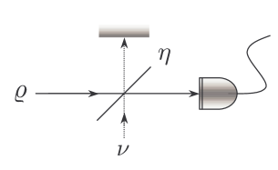
Figure 5.1: Model of a realistic on/off photodetector with non-unit quantum efficiency $\eta$, and non-zero dark counts.

As mentioned above, in a photodetector each photon ionizes a single atom and, at least in principle, the resulting charge is amplified to produce a measurable pulse. Taking into account the quantum efficiency, we conclude that the resulting current is proportional to the incoming photon flux and thus we have a linear detector. On the other hand, detectors operating at very low intensities resort to avalanche process in order to transform a single ionization event into a recordable pulse. This implies that one cannot discriminate between a single photon or many photons as the outcomes from such detectors are either a click, corresponding to any number of photons, or nothing which means that no photons have been revealed. These Geiger-like detectors are often referred to as on/off detectors. For unit quantum efficiency, the action of an on/off detector is described by the two-value POVM $\{\Pi_{0}\doteq|0\rangle\langle 0|,\Pi_{1}\doteq{\mathbb{I}}-\Pi_{0}\}$, which represents a partition of the Hilbert space of the signal. In the realistic case, when an incoming photon is not detected with unit probability, the POVM is given by

$$\Pi_{0}(\eta)=\sum_{k=0}^{\infty}(1-\eta)^{k}\>|k\rangle\langle k|\,,\qquad\Pi_{1}(\eta)={\mathbb{I}}-\Pi_{0}(\eta)\;,$$ (5.20)

with $\eta$ denoting quantum efficiency. The corresponding characteristic and the Wigner functions can be easily obtained from that of a number state [see Eqs. (5.15a) and (5.15b)]. We have

$$\chi[\Pi_{0}(\eta)](\lambda) =\frac{1}{\eta}\>\exp\left\{-\frac{2-\eta}{2\eta}\,|\lambda|^{2}\right\}\,,\quad\chi[\Pi_{1}(\eta)](\lambda)=\pi\delta^{(2)}(\lambda)-\chi[\Pi_{0}(\eta)](\lambda)\>,$$ (5.21a)

$$W[\Pi_{0}(\eta)](\alpha) =\frac{1}{\pi}\frac{2}{2-\eta}\exp\left\{-\frac{2\eta}{2-\eta}\,|\alpha|^{2}\right\}\,,\quad W[\Pi_{1}(\eta)](\alpha)=\frac{1}{\pi}-W[\Pi_{0}(\eta)](\alpha)\;.$$ (5.21b)

Besides quantum efficiency, i.e. lost photons, the performance of a realistic photodetector are also degraded by the presence of dark-count, namely by “clicks” that do not correspond to any incoming photon. In order to take into account both these effects we use the simple scheme introduced in the previous Section and depicted in Fig. 5.1. A real photodetector is modeled as an ideal photodetector (unit quantum efficiency, no dark-count) preceded by a beam splitter of transmissivity equal to the quantum efficiency $\eta$, whose second port is in an auxiliary excited state $\nu$, which can be a thermal state, or a phase-averaged coherent state, depending on the kind of background noise (thermal or Poissonian) we would like to describe. When the second port of the beam splitter is the vacuum $\nu=|0\rangle\langle 0|$, we have no dark-counts and the POVM of the photodetector reduces to that of Eq. (5.20). On the other hand, when the second port of the BS excited in a generic mixture

$$\nu=\sum_{s}\nu_{ss}|s\rangle\langle s|\>,$$

then the overall POVM describing the on/off photodetection is expressed as the following generalized convolution

$$\Pi_{0}^{\nu}(\eta)=\hbox{Tr}_{b}\left[U_{\phi}\varrho\otimes\nu\>U^{\dagger}_{\phi}\>\mathbb{I}\otimes|0\rangle\langle 0|\right]=\sum_{n=0}^{\infty}(1-\eta)^{n}\sum_{s=0}^{\infty}\nu_{ss}\>\eta^{s}\>\binom{n+s}{s}\>|n\rangle\langle n|\;,$$ (5.22)

whereas the characteristic and the Wigner functions read as follows

$$\chi[\Pi_{0}^{\nu}(\eta)](\lambda) =\frac{1}{\eta}\exp\left\{-\frac{2-\eta}{\eta}\,|\lambda|^{2}\right\}\sum_{s=0}^{\infty}\nu_{ss}\,L_{s}\left(\frac{(1-\eta)|\lambda|^{2}}{2\eta}\right)\,,$$ (5.23a)

$$W[\Pi_{0}^{\nu}(\eta)](\alpha) =\frac{2}{\pi}\exp\left\{-\frac{2\eta}{2-\eta}\,|\alpha|^{2}\right\}\sum_{s=0}^{\infty}\nu_{ss}\>\frac{\eta^{s}}{(2-\eta)^{1+s}}\>L_{s}\left(\frac{4(\eta-1)|\alpha|^{2}}{2-\eta}\right)\>.$$ (5.23b)

The density matrices of a thermal state and a phase-averaged coherent state (with $n_{b}$ mean photons) are given by

$$\nu_{t}=\frac{1}{n_{b}+1}\sum_{s=0}^{\infty}\left(\frac{n_{b}}{n_{b}+1}\right)^{s}\>|s\rangle\langle s|\,,\qquad\nu_{p}=e^{-n_{b}}\sum_{s=0}^{\infty}\frac{(n_{b})^{s}}{s!}\,|s\rangle\langle s|\;.$$ (5.24)

In order to reproduce a background noise with mean photon number $N$ we consider the state $\nu$ with average photon number $n_{b}=N/(1-\eta)$. In this case we have

$$\Pi_{0}^{t}(\eta,N) =\frac{1}{1+N}\sum_{n=0}^{\infty}\left(1-\frac{\eta}{1+N}\right)^{n}\>|n\rangle\langle n|\,,$$ (5.25a)

$$\Pi_{0}^{p}(\eta,N) =e^{-N}\sum_{n=0}^{\infty}(1-\eta)^{n}\>L_{n}\left(-\frac{\eta N}{1-\eta}\right)\>|n\rangle\langle n|\;,$$ (5.25b)

where $t$ and $p$ denotes thermal and Poissonian respectively. The corresponding characteristic and Wigner function are given by

$$\chi[\Pi_{0}^{t}(\eta,N)](\lambda) =\frac{1}{\eta}\exp\left\{-\frac{2(1+N)-\eta}{2\eta}\,|\lambda|^{2}\right\}\,,$$ (5.26a)

$$\chi[\Pi_{0}^{p}(\eta,N)](\lambda) =\frac{1}{\eta}\exp\left\{-\frac{2-\eta}{2\eta}\,|\lambda|^{2}\right\}I_{0}\left(2\sqrt{-\frac{N}{\eta}|\lambda|^{2}}\right)$$ (5.26b)

and

$$W[\Pi_{0}^{t}(\eta,N)](\alpha) =\frac{1}{\pi}\frac{2}{2(1+N)-\eta}\exp\left\{-\frac{2\eta}{2(1+N)-\eta}\,|\alpha|^{2}\right\}\,,$$ (5.27a)

$$W[\Pi_{0}^{p}(\eta,N)](\alpha) =\frac{1}{\pi}\>\frac{2}{2-\eta}\exp\left\{-\frac{2\eta}{2-\eta}(N+|\alpha|^{2})\right\}\>I_{0}\left(\frac{4|\alpha|\sqrt{\eta N}}{2-\eta}\right)\;,$$ (5.27b)

respectively, where $I_{0}(x)$ is the $0$-th modified Bessel function of the first kind.

5.4 Application: de-Gaussification by vacuum removal

As we have already pointed out, Gaussian states are very important for continuous variable quantum information. However, there are situations, as for example in testing nonlocality with feasible measurements (see Chapter 6), where one needs to go beyond Gaussian states. Indeed, when the Gaussian character is lost, then immediately the Wigner function of the state becomes negative, for pure states, hence stronger nonclassical properties should emerge. An effective method to “de-Gaussify” a state is through a conditional measurement, and, in particular, by elimination of its vacuum component leading to a state which is necessarily described by a negative Wigner function. In the next two Sections this strategy will be applied both to the TWB and the tripartite state $|T\rangle$ given in Eq. (2.49) through the on/off detection scheme introduced in the previous Section.

5.4.1 De-Gaussification of TWB: the IPS map

In this Section we address a de-Gaussification process onto the twin-beam state (TWB) of two modes of radiation $|\Lambda\rangle\rangle_{ab}=\sqrt{1-\lambda^{2}}\,\sum_{n=0}^{\infty}\,\lambda^{n}|n,n\rangle_{ab}$, where we assume the TWB parameter $\lambda=\tanh r$ as real, $r$ being referred to as the squeezing parameter. The corresponding Wigner function is given by

$$W_{r}(\alpha,\beta)=\frac{4}{\pi^{2}}\exp\{-2A(|\alpha|^{2}+|\beta|^{2})+2B(\alpha\beta+\alpha^{*}\beta^{*})\}\,,$$ (5.28)

with $A\equiv A(r)=\cosh(2r)$ and $B\equiv B(r)=\sinh(2r)$.

The de-Gaussification of a TWB can be achieved by subtracting photons from both modes through on/off detection [92, 93, 94]. Since the scheme does not discriminate the number of subtracted photons, we will refer to this process as to inconclusive photon subtraction (IPS).

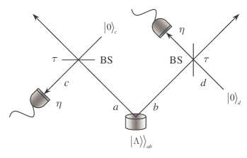
Figure 5.2: Scheme of the IPS process.

The IPS scheme is sketched in Fig. 5.2. The modes $a$ and $b$ of the TWB are mixed with vacuum modes at two unbalanced beam splitters (BS) with equal transmissivity $\tau=\cos^{2}\phi$; the reflected modes $c$ and $d$ are then revealed by avalanche photodetectors (APD) with equal efficiency $\eta$. APD’s can only discriminate the presence of radiation from the vacuum. The positive operator-valued measure (POVM) $\{\Pi_{0}(\eta),\Pi_{1}(\eta)\}$ of each detector is given in Eq. (5.20). Overall, the conditional measurement on modes $c$ and $d$, is described by the POVM (assuming equal quantum efficiency for the photodetectors)

$${\Pi}_{00}(\eta) ={\Pi}_{0,c}(\eta)\otimes{\Pi}_{0,d}(\eta)\,,\qquad\qquad{\Pi}_{01}(\eta)={\Pi}_{0,c}(\eta)\otimes{\Pi}_{1,d}(\eta)\>,$$ (5.29a)

$${\Pi}_{10}(\eta) ={\Pi}_{1,c}(\eta)\otimes{\Pi}_{0,d}(\eta)\,,\qquad\qquad{\Pi}_{11}(\eta)={\Pi}_{1,c}(\eta)\otimes{\Pi}_{1,d}(\eta)\;.$$ (5.29b)

When the two photodetectors jointly click, the conditioned output state of modes $a$ and $b$ is given by [92, 95]

$$\mathcal{E}(R)=\frac{\hbox{Tr}_{cd}\big{[}U_{ac}(\phi)\otimes U_{bd}(\phi)\>R\otimes|0\rangle_{c}{}_{c}\langle 0|\otimes|0\rangle_{d}{}_{d}\langle 0|\>U_{ac}^{{\dagger}}(\phi)\otimes U_{bd}^{{\dagger}}(\phi)\>{\mathbb{I}}_{a}\otimes{\mathbb{I}}_{b}\otimes{\Pi}_{11}(\eta)\big{]}}{p_{11}(r,\phi,\eta)}\>,$$ (5.30)

where $U_{ac}(\phi)=\exp\{-\phi(a^{{\dagger}}c-ac^{{\dagger}})\}$ and $U_{bd}(\phi)$ are the evolution operators of the beam splitters and $R$ the density operator of the two-mode state entering the beam splitters (in our case $R=\varrho_{\hbox{\tiny TWB}}=|\Lambda\rangle\rangle_{ab}{}_{ba}\langle\langle\Lambda|$). The partial trace on modes $c$ and $d$ can be explicitly evaluated, thus arriving at the following decomposition of the IPS map . We have

$$\mathcal{E}(R)=\frac{1}{p_{11}(r,\phi,\eta)}\>\sum_{p,q=1}^{\infty}\>m_{p}(\phi,\eta)\>M_{pq}(\phi)\>R\>M_{pq}^{{\dagger}}(\phi)\>m_{q}(\phi,\eta)\>$$ (5.31)

where

$$m_{p}(\phi,\eta)={\displaystyle\frac{\tan^{2p}\phi\,\,[1-(1-\eta)^{p}]}{p!}}\,,\qquad M_{pq}(\phi)=\frac{\mbox{}}{\mbox{}}a^{p}b^{q}\,(\cos\phi)^{a^{\dagger}a+b^{\dagger}b}\,.$$ (5.32)

Now we explicitly calculate the Wigner function of the state $\varrho_{\hbox{\tiny{IPS}}}=\mathcal{E}(\varrho_{\hbox{\tiny TWB}})$, which, as one may expect, is no longer Gaussian and positive-definite. The state entering the two beam splitters is described by the Wigner function

$$W_{r}^{\hbox{\tiny(in)}}(\alpha,\beta,\zeta,\xi)=W_{r}(\alpha,\beta)\,\frac{4}{\pi^{2}}\exp\left\{-2|\zeta|^{2}-2|\xi|^{2}\right\}\,,$$ (5.33)

where the second factor at the right hand side represents the two vacuum states of modes $c$ and $d$. The action of the beam splitters on $W^{\hbox{\tiny(in)}}_{r}$ can be summarized by the following change of variables (see Section 1.4.2)

$$\alpha \to\alpha\cos\phi+\zeta\sin\phi\,,\quad\zeta\to\zeta\cos\phi-\alpha\sin\phi\,,$$ (5.34a)

$$\beta \to\beta\cos\phi+\xi\sin\phi\,,\quad\xi\to\xi\cos\phi-\beta\sin\phi\,,$$ (5.34b)

and the output state, after the beam splitters, is then given by

$$W_{r,\phi}^{\hbox{\tiny(out)}}(\alpha,\beta,\zeta,\xi)=\frac{4}{\pi^{2}}\,W_{r,\phi}(\alpha,\beta)\,\exp\left\{-a|\xi|^{2}+w\xi+w^{*}\xi^{*}\right\}\\ \times\exp\big{\{}-a|\zeta|^{2}+(v+2B\xi\sin^{2}\phi)\zeta+(v^{*}+2B\xi^{*}\sin^{2}\phi)\zeta^{*}\big{\}}\,,$$ (5.35)

where

$$W_{r,\phi}(\alpha,\beta)=\frac{4}{\pi^{2}}\,\exp\left\{-b(|\alpha|^{2}+|\beta|^{2})+2B\cos^{2}\phi\,(\alpha\beta+\alpha^{*}\beta^{*})\right\}$$ (5.36)

and

$$a \equiv a(r,\phi)=2(A\sin^{2}\phi+\cos^{2}\phi),$$ (5.37a)

$$b \equiv b(r,\phi)=2(A\cos^{2}\phi+\sin^{2}\phi)\,,$$ (5.37b)

$$v \equiv v(r,\phi)=2\cos\phi\,\sin\phi\,[(1-A)\alpha^{*}+B\beta],$$ (5.37c)

$$w \equiv w(r,\phi)=2\cos\phi\,\sin\phi\,[(1-A)\beta^{*}+B\alpha]\,.$$ (5.37d)

At this stage on/off detection is performed on modes $c$ and $d$ (see Fig. 5.2). We are interested in the situation when both the detectors click. The Wigner function of the double click element $\Pi_{11}(\eta)$ of the POVM [see Eq. (5.29)] is given by [92, 96]

$$W_{\eta}(\zeta,\xi)\equiv W[\Pi_{11}(\eta)](\zeta,\xi)=\frac{1}{\pi^{2}}\{1-Q_{\eta}(\zeta)-Q_{\eta}(\xi)+Q_{\eta}(\zeta)Q_{\eta}(\xi)\}\,,$$ (5.38)

with

$$Q_{\eta}(z)=\frac{2}{2-\eta}\,\exp\Bigg{\{}-\frac{2\eta}{2-\eta}\,|z|^{2}\Bigg{\}}\,.$$ (5.39)

Using Eq. (5.30) and the phase-space expression of trace for each mode [see Eq. (1.133)], the Wigner function of the output state, conditioned to the double click event, reads

$$W_{r,\phi,\eta}(\alpha,\beta)=\frac{f(\alpha,\beta)}{p_{11}(r,\phi,\eta)}\,,$$ (5.40)

where $f(\alpha,\beta)\equiv f_{r,\phi,\eta}(\alpha,\beta)$ with

$$f(\alpha,\beta)=\pi^{2}\,\int_{\mathbb{C}^{2}}d^{2}\zeta\,d^{2}\xi\,\frac{4}{\pi^{2}}\,W_{r,\phi}(\alpha,\beta)\,\sum_{k=1}^{4}\frac{C_{k}(\eta)}{\pi^{2}}\,G_{r,\phi,\eta}^{(k)}(\alpha,\beta,\zeta,\xi)\,,$$ (5.41)

and $p_{11}(r,\phi,\eta)$ is the double-click probability reported above, which can be written as function of $f(\alpha,\beta)$ as follows

$$p_{11}(r,\phi,\eta)=\pi^{2}\,\int_{\mathbb{C}^{2}}d^{2}\alpha\,d^{2}\beta\,f(\alpha,\beta)\,.$$ (5.42)

The quantities $G_{r,\phi,\eta}^{(k)}(\alpha,\beta,\zeta,\xi)$ in Eq. (5.41) are given by

$$G_{r,\phi,\eta}^{(k)}(\alpha,\beta,\zeta,\xi)=\exp\big{\{}-x_{k}|\zeta|^{2}+(v+2B\xi\sin^{2}\phi)\zeta+(v^{*}+2B\xi^{*}\sin^{2}\phi)\zeta^{*}\big{\}}\\ \times\exp\left\{-y_{k}|\xi|^{2}+w\xi+w^{*}\xi^{*}\right\}\,,$$ (5.43)

where the expressions of $x_{k}\equiv x_{k}(r,\phi,\eta)$, $y_{k}\equiv y_{k}(r,\phi,\eta)$, and $C_{k}(\eta)$ are reported in Table 5.1.

$k$	$x_{k}(r,\phi,\eta)$	$y_{k}(r,\phi,\eta)$	$C_{k}(\eta)$
1	$a$	$a$	1
2	${\displaystyle a+\frac{2}{2-\eta}}$	$a$	${\displaystyle-\frac{2}{2-\eta}}$
3	$a$	${\displaystyle a+\frac{2}{2-\eta}}$	${\displaystyle-\frac{2}{2-\eta}}$
4	${\displaystyle a+\frac{2}{2-\eta}}$	${\displaystyle a+\frac{2}{2-\eta}}$	${\displaystyle\left(\frac{2}{2-\eta}\right)^{2}}$

Table 5.1: Expressions of $C_{k}$, $x_{k}$, and $y_{k}$ appearing in Eq. (5.43).

The mixing with the vacuum in a beam splitter with transmissivity $\tau$ followed by on/off detection with quantum efficiency $\eta$ is equivalent to mixing with an effective transmissivity [92]

$$\tau_{\rm eff}\equiv\tau_{\rm eff}(\phi,\eta)=1-\eta(1-\tau)$$ (5.44)

followed by an ideal (i.e. efficiency equal to 1) on/off detection. Therefore, the state (5.40) can be studied for $\eta=1$ and replacing $\tau=\cos^{2}\phi=1-\sin^{2}\phi$ with $\tau_{\rm eff}$. Thanks to this substitution, after the integrations we have

$$f(\alpha,\beta)=\frac{1}{\pi^{2}}\,\sum_{k=1}^{4}\frac{16\,C_{k}}{x_{k}y_{k}-4B^{2}(1-\tau_{\rm eff})^{2}}\\ \times\exp\{(f_{k}-b)|\alpha|^{2}+(g_{k}-b)|\beta|^{2}+(2B\tau_{\rm eff}+h_{k})(\alpha\beta+\alpha^{*}\beta^{*})\}$$ (5.45)

and

$$p_{11}(r,\tau_{\rm eff})=\sum_{k=1}^{4}\frac{16\,[x_{k}y_{k}-4B^{2}(1-\tau_{\rm eff})^{2}]^{-1}\,C_{k}}{(b-f_{k})(b-g_{k})-(2B\tau_{\rm eff}+h_{k})^{2}}\,,$$ (5.46)

where we defined $C_{k}\equiv C_{k}(1)$ and

$$f_{k} \equiv f_{k}(r,\tau_{\rm eff})=N_{k}\,[x_{k}B^{2}+4B^{2}(1-A)(1-\tau_{\rm eff})+y_{k}(1-A)^{2}]\,,$$ (5.47a)

$$g_{k} \equiv g_{k}(r,\tau_{\rm eff})=N_{k}\,[x_{k}(1-A)^{2}+4B^{2}(1-A)(1-\tau_{\rm eff})+y_{k}B^{2}]\,,$$ (5.47b)

$$h_{k} \equiv h_{k}(r,\tau_{\rm eff})=N_{k}\,[(x_{k}+y_{k})B(1-A)+2B(B^{2}+(1-A)^{2})(1-\tau_{\rm eff})]\,,$$ (5.47c)

$$N_{k} \equiv N_{k}(r,\tau_{\rm eff})={\displaystyle\frac{4\tau_{\rm eff}\,(1-\tau_{\rm eff})}{x_{k}y_{k}-4B^{2}(1-\tau_{\rm eff})^{2}}\,.}$$ (5.47d)

In this way, the Wigner function of the IPS state can be rewritten as

$$W_{\hbox{\rm\tiny IPS}}(\alpha,\beta)=\frac{4}{\pi^{2}}\frac{1}{p_{11}(r,\tau_{\rm eff})}\sum_{k=1}^{4}{\cal C}_{k}\,W_{k}(\alpha,\beta)\,,$$ (5.48)

where we introduced

$${\cal C}_{k}\equiv{\cal C}_{k}(r,\tau_{\rm eff})=\frac{4\,C_{k}}{x_{k}y_{k}-4B^{2}(1-\tau_{\rm eff})^{2}}\,,$$ (5.49)

and defined

$$W_{k}(\alpha,\beta)=\exp\{(f_{k}-b)|\alpha|^{2}+(g_{k}-b)|\beta|^{2}+(2B\tau_{\rm eff}+h_{k})(\alpha\beta+\alpha^{*}\beta^{*})\}\,.$$ (5.50)

Finally, the density matrix corresponding to $W_{\hbox{\rm\tiny IPS}}(\alpha,\beta)$ reads as follows [92]

$${\varrho}_{\hbox{\rm\tiny IPS}}=\frac{1-\lambda^{2}}{p_{11}(r,\tau_{\rm eff})}\sum_{n,m=0}^{\infty}(\lambda\,\tau_{\rm eff})^{n+m}\\ \times\sum_{h,k=0}^{{\rm Min}[n,m]}\left(\frac{1-\tau_{\rm eff}}{\tau_{\rm eff}}\right)^{h+k}\sqrt{{n\choose h}{n\choose k}{m\choose h}{m\choose k}}\times|n-k\rangle_{a}|n-h\rangle_{b}{{}_{b}}\langle m-h|{{}_{a}}\langle m-k|\,,$$ (5.51)

with $\lambda=\tanh r$.

The state given in Eq. (5.48) is no longer a Gaussian state. Its use in the enhancement of the nonlocality [97, 98, 95] and in the improvement of CV teleportation [92] will be investigated in Chapter 6 and 7, respectively.

5.4.2 De-Gaussification of tripartite state: the TWBA state

In this Section we consider the tripartite state $|T\rangle$ given in Eq. (2.49) as a source of two-mode states. In particular, we analyze two-mode non-Gaussian state obtained by a conditional measurement performed on it. Due to the structure of the state $|T\rangle$, its vacuum component can be subtracted by a conditional measurement on mode $a_{3}$, the same observation being valid for mode $a_{2}$. Let us consider on/off detection performed on mode $a_{3}$. The three-mode two-valued POVM is $\{\Pi_{0}^{(3)}(\eta),\Pi_{1}^{(3)}(\eta)\}$, with the element associated to the “no photons” result given by

$$\Pi_{0}^{(3)}(\eta)\doteq\mathbb{I}_{1}\otimes\mathbb{I}_{2}\otimes\sum_{n=0}^{\infty}(1-\eta)^{n}|n\rangle_{3}{}_{3}\langle n|\>.$$ (5.52)

The probability of a “click” is

$$P_{1}\equiv P_{1}(N_{3},\eta)=\hbox{Tr}_{123}\left[|T\rangle\langle T|\>\Pi_{1}^{(3)}(\eta)\right]=\frac{\eta N_{3}}{(1+\eta N_{3})}\>,$$ (5.53)

while the conditional output state reads as follows

$$\varrho_{\hbox{\tiny TWBA}} =\frac{1}{P_{1}}\hbox{Tr}_{3}\left[|T\rangle\langle T|\>\Pi_{1}^{(3)}(\eta)\right]$$

$$=\frac{1+\eta N_{3}}{(1+N_{1}+N_{2})\eta N_{3}}\,\sum_{p=1}^{\infty}\left(\frac{N_{3}}{1+N_{1}}\right)^{p}\frac{1-(1-\eta)^{p}}{p!}(a^{\dagger}_{1})^{p}\,|\Lambda\rangle\rangle_{12}{}_{21}\langle\langle\Lambda|a^{p}_{1}\>,$$ (5.54)

where we denote by $|\Lambda\rangle\rangle_{12}$ the TWB state of the modes $a_{1}$ and $a_{2}$ with parameter $\lambda=\sqrt{N_{2}/(1+N_{1})}$ (see Section 1.4.4). We indicated this state with a subscript TWBA (i.e. TWB added) since it corresponds to a mixture of TWBs with additional photons in one of the modes. In order to evaluate its Wigner function we use (5.21a) for the characteristic function of $\Pi_{1}^{(3)}(\eta)$, hence the characteristic function of $\varrho_{\hbox{\tiny TWBA}}$ is given by

$$\chi[\varrho_{\hbox{\tiny TWBA}}](\lambda_{1},\lambda_{2})=\frac{1}{P_{1}}\Bigg{\{}\chi[|T\rangle\langle T|](\lambda_{1},\lambda_{2},0)-\frac{1}{\eta}\int_{\mathbb{C}}\frac{d^{2}\mu}{\pi}\chi[|T\rangle\langle T|](\lambda_{1},\lambda_{2},\mu)\exp\left\{-\frac{2-\eta}{2\eta}\,|\mu|^{2}\right\}\Bigg{\}}\;.$$ (5.55)

After some algebra the Wigner function associated with state $\varrho_{\hbox{\tiny TWBA}}$ can now be calculated. It reads as follows

$$W_{\hbox{\tiny TWBA}}({\boldsymbol{Y}})=\frac{1+\eta N_{3}}{4\eta N_{3}}\>\left(\frac{2}{\pi}\right)^{2}\Bigg{\{}\frac{1}{\sqrt{{\rm Det}\,[{\boldsymbol{V}}_{T}^{\prime}]}}\exp\left\{-{\boldsymbol{Y}}^{\scriptscriptstyle T}\left({\boldsymbol{V}}_{T}^{\prime}\right)^{-1}{\boldsymbol{Y}}\right\}\\ -\frac{1}{\eta}\frac{2}{\sqrt{{\rm Det}\,[{\boldsymbol{D}}]}}\exp\left\{-{\boldsymbol{Y}}^{\scriptscriptstyle T}\left({{\boldsymbol{D}}}^{-1}\right)^{\prime}{\boldsymbol{Y}}\right\}\Bigg{\}}\;,$$ (5.56)

where ${\boldsymbol{Y}}=(x_{1},x_{2},y_{1},y_{2})^{\scriptscriptstyle T}$, and ${{\boldsymbol{D}}}={{\boldsymbol{V}}_{T}}+{\rm Diag}(0,0,\frac{2-\eta}{\eta},0,0,\frac{2-\eta}{\eta})$, ${\boldsymbol{V}}_{T}$ being defined in Eq. (2.51). In order to simplify the notation we have indicated with ${{\boldsymbol{O}}}^{\prime}$ the $4\times 4$ matrix obtained from the $6\times 6$ matrix ${{\boldsymbol{O}}}$ deleting the elements corresponding to the third mode (3-rd row/column and 6-th row/column), due to the trace over the 3-rd mode. Nonlocality properties of the TWBA state will investigated in Chapter 6.

5.5 Homodyne detection

Homodyne detection schemes are devised to provide the measurement of a single-mode quadrature $x_{\phi}$ through the mixing of the signal under investigation with a highly excited classical field at the same frequency, referred to as the local oscillator (LO). Homodyne detection was proposed for the radiation field in Ref. [99], and subsequently demonstrated in Ref. [100]. For the radiation field quadrature measurements can be achieved by balanced and unbalanced homodyne schemes, whereas realizations for atomic systems have also been proposed [101].

5.5.1 Balanced homodyne detection

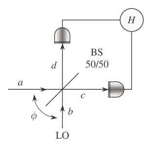
Figure 5.3: Schematic diagram of the balanced homodyne detector.

The schematic diagram of a balanced homodyne detector is reported in Fig. 5.3. The signal mode $a$ interferes with a second mode $b$ excited in a coherent semiclassical state (e.g. a laser beam) in a balanced (50/50) beam splitter (BS). The mode $b$ is the LO mode of the detector. It operates at the same frequency of $a$, and is excited in a coherent state $|z\rangle$ with large amplitude $z$. The BS is tuned to have real coupling, hence no additional phase-shift is imposed on the reflected and transmitted beams. Moreover, since in all experiments that use homodyne detectors the signal and the LO beams are generated by a common source, we assume that they have a fixed phase relation. In this case the LO phase provides a reference for the quadrature measurement, namely we identify the phase of the LO with the phase difference between the two modes. As we will see, by tuning $\phi=\arg[z]$ we can measure the quadrature $x_{\phi}$ at different phases $\phi$. After the BS the two modes are detected by two identical photodetectors (usually linear photodiodes), and finally the difference of photocurrents at zero frequency is electronically processed and rescaled by $2|z|$. According to Eqs. (1.75) and (1.90), denoting by $c$ and $d$ the output mode from the beam splitter, the resulting homodyne photocurrent $H$ is given by

$$H={\frac{c^{{\dagger}}c-d^{{\dagger}}d}{2|z|}}=\frac{{a^{\dagger}}b+b^{{\dagger}}a}{2|z|}\;.$$ (5.57)

Notice that the spectrum of the operators ${a^{\dagger}}b+b^{{\dagger}}a$ is discrete and coincides with the set ${\mathbb{Z}}$ of relative integers. Therefore the spectrum of the homodyne photocurrent $H$ is discrete too, approaching the real axis in the limit of highly excited LO ($|z|\gg 1$). We now exploit the assumption of a LO excited in a strong semiclassical state, i.e. we neglect fluctuations of the LO and make the substitutions $b\rightarrow z$, $b^{\dagger}\rightarrow z^{*}$. The moments of the homodyne photocurrent are then given by

$$H=x_{\phi}\,,\qquad H^{2}=x^{2}_{\phi}+\frac{a^{\dagger}a}{4|z|^{2}}\,,\qquad\cdots\mbox{}\qquad H^{n}=x^{2n-2}_{\phi}\>\left(x^{2}_{\phi}+\frac{a^{\dagger}a}{4|z|^{2}}\right)\;,$$ (5.58)

which coincide with the quadrature moments for signals satisfying $\langle a^{\dagger}a\rangle\ll 4|z|^{2}$. In this limit the distribution of the outcomes $h$ of the homodyne photocurrent is equal to that of the corresponding field quadratures. The POVM $\{\Pi_{h}\}$ of the detector coincides with the spectral measure of the quadratures

$$\Pi_{h}\xrightarrow{|z|\gg 1}\Pi(x)=|x\rangle_{\phi}{}_{\phi}\langle x|\equiv\delta(x_{\phi}-x)\>,$$ (5.59)

i.e. the projector on the eigenstate of the quadrature $x_{\phi}$ with eigenvalue $x$. In conclusion, the balanced homodyne detector achieves the ideal measurement of the quadrature $x_{\phi}$ in the strong LO regime. In this limit, which summarizes the two conditions i) $|z|\gg 1$ to have a continuous spectrum and ii) $|z|^{2}\gg\langle a^{\dagger}a\rangle$ to neglect extra terms in the photocurrent moments, the probability distribution of the output photocurrent $H$ approaches the probability distribution $p(x,\phi)={}_{\phi}\langle x|\varrho|x\rangle_{\phi}$ of the quadrature $x_{\phi}$ for of the signal mode $a$. The same result [102] can be obtained by evaluating the moment generating function $M_{H}(\mu)=\hbox{Tr}\left[\varrho\otimes|z\rangle\langle z|\>e^{i\mu H}\right]$. Using the disentangling formula for ${\rm SU}(2)$ (1.68) we have

$$M_{H}(\mu)=\left\langle e^{i\tan\left({\frac{\mu}{2|z|}}\right)b^{{\dagger}}a}\left[\cos\left({\frac{\mu}{2|z|}}\right)\right]^{{a^{\dagger}}a-b^{{\dagger}}b}e^{i\tan\left({\frac{\mu}{2|z|}}\right){a^{\dagger}}b}\right\rangle_{ab}\;.$$ (5.60)

Since mode $b$ is in a coherent state $|z\rangle$ the partial trace over $b$ can be evaluated as follows

$$M_{H}(\mu)=\left\langle e^{i\tan\left({\frac{\mu}{2|z|}}\right)z^{*}a}\left[\cos\left({\frac{\mu}{2|z|}}\right)\right]^{{a^{\dagger}}a}e^{i\tan\left({\frac{\mu}{2|z|}}\right)z{a^{\dagger}}}\right\rangle_{a}\left\langle z\Bigg{|}\left[\cos\left({\frac{\mu}{2|z|}}\right)\right]^{-b^{{\dagger}}b}\Bigg{|}z\right\rangle\;.$$ (5.61)

Now, rewriting (5.61) in normal order with respect to mode $a$ we have

$$M_{H}(\mu)=\left\langle e^{iz\sin\left({\frac{\mu}{2|z|}}\right){a^{\dagger}}}\exp\left\{-2\sin^{2}\left({\frac{\mu}{4|z|}}\right)({a^{\dagger}}a+|z|^{2})\right\}e^{iz^{*}\sin\left({\frac{\mu}{2|z|}}\right)a}\right\rangle_{a}\!\!.$$ (5.62)

In the strong LO limit (5.62) becomes

$$\lim_{z\to\infty}M_{H}(\mu)=\left\langle e^{i{\frac{\mu}{2}}e^{i\phi}{a^{\dagger}}}\,\exp\left\{\frac{-\mu^{2}}{8}\right\}\,e^{i{\frac{\mu}{2}}e^{-i\phi}a}\right\rangle_{a}=\left\langle\exp\left\{i\mu x_{\phi}\right\}\right\rangle_{a}\;.$$ (5.63)

The generating function in (5.63) then corresponds to the POVM

$$\Pi(x)=\int_{\mathbb{R}}{\frac{d\mu}{2\pi}}\,\exp\{i\mu(x_{\phi}-x)\}=\delta(x_{\phi}-x)\equiv|x\rangle_{\phi}{}_{\phi}\langle x|\;,$$ (5.64)

which confirm the conclusions drawn in Eq. (5.59).

In order to take into account non-unit quantum efficiency at detectors we employ the model introduced in the previous Sections, i.e. each inefficient detector is viewed as an ideal detector preceded by a beam splitter of transmissivity $\eta$ with the second port left in the vacuum. The homodyne photocurrent is again formed as the difference photocurrent, now rescaled by $2|z|\eta$. We have

$$H_{\eta}\simeq\frac{1}{2|z|}\left\{\left[a+\sqrt{\frac{1-\eta}{2\eta}}(u+v)\right]b^{\dagger}+h.c.\right\}\;,$$ (5.65)

where only terms containing the strong LO mode $b$ are retained, and $u$ and $v$ denote the additional vacuum modes introduced to describe loss of photons. The POVM is obtained by replacing

$$x_{\phi}\rightarrow x_{\phi}+\sqrt{\frac{1-\eta}{2\eta}}(u_{\phi}+v_{\phi})\;$$ (5.66)

in Eqs. (5.64), with $w_{\phi}=\frac{1}{2}(w^{\dagger}e^{i\phi}+we^{-i\phi})$, $w=u,v$, and tracing the vacuum modes $u$ and $v$. One then obtains

$$\Pi_{\eta}(x) =\frac{1}{\sqrt{2\pi\delta^{2}_{\eta}}}\>\exp\left\{-\frac{(x_{\phi}-x)^{2}}{2\delta_{\eta}^{2}}\right\}$$

$$=\frac{1}{\sqrt{2\pi\delta^{2}_{\eta}}}\int_{\mathbb{C}}dy\,\exp\left\{-\frac{(x-y)^{2}}{2\delta_{\eta}^{2}}\right\}|y\rangle_{\phi}{}_{\phi}\langle y|\;,$$ (5.67)

where

$$\delta_{\eta}^{2}=\frac{1-\eta}{4\eta}\;.$$ (5.68)

Thus the POVMs, and in turn the probability distribution of the output photocurrent, are just the Gaussian convolutions of the ideal ones.

The Wigner functions of the homodyne POVM is given by

$$W[\Pi_{\eta}(x)](\alpha)=\frac{1}{\sqrt{2\pi\delta^{2}_{\eta}}}\exp\left\{-\frac{[x-\frac{1}{2}(\alpha e^{-i\phi}+\alpha^{*}e^{i\phi})]^{2}}{2\delta_{\eta}^{2}}\right\}\>,$$ (5.69)

which leads to $W[\Pi(x)](\alpha)\xrightarrow{\eta\rightarrow 1}\delta(x-\frac{1}{2}(\alpha e^{-i\phi}+\alpha^{*}e^{i\phi}))$ in the limit of an ideal homodyne detector.

5.5.2 Unbalanced homodyne detection

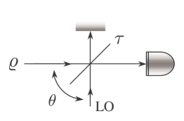
Figure 5.4: Schematic diagram of unbalanced homodyne detector.

The scheme of Fig. 5.4 is known as unbalanced homodyne detector and represents an alternative method to measure the statistics of a field quadrature. The signal under investigation is mixed with the LO at a beam splitter with transmissivity $\tau=\cos^{2}\phi$. The reflected beam is then absorbed, whereas the transmitted beam is revealed through a linear photocounter. If $a$ is the signal mode and $b$ the LO mode the transmitted mode $c$ can be written as $c=a\cos\phi+b\sin\phi$. The detected photocurrent is given by

$$n_{c} \equiv c^{\dagger}c=a^{\dagger}a\cos^{2}\phi+b^{\dagger}b\sin^{2}\phi+(a^{\dagger}b+b^{\dagger}a)\sin\phi\cos\phi\>$$ (5.70)

and the unbalanced homodyne photocurrent is obtained by a simple rescaling

$$I_{H}=\frac{n_{c}}{2\sin^{2}\phi|z|}\>,$$

where $z$ is again the LO amplitude. Upon tracing over the local oscillator, in the limit of $|z|\gg\langle a^{\dagger}a\rangle$, we have for the first two moments

$$\langle I_{H}\rangle =\frac{1}{2}+\frac{1}{|z|\tan\phi}\langle x_{\theta}\rangle+O(|z|^{-2})\,,$$ (5.71)

$$\langle I_{H}^{2}\rangle =\frac{1}{4}+\frac{1}{|z|\tan\phi}\langle x_{\theta}\rangle+\frac{1}{|z|^{2}\tan^{2}\phi}\langle x^{2}_{\theta}\rangle+O(|z|^{-2})\;,$$ (5.72)

and therefore $\langle\Delta I^{2}_{H}\rangle=(|z|^{2}\tan^{2}\phi)^{-1}\langle\Delta x^{2}_{\theta}\rangle$, where $\theta$ is the shift between signal and LO. The procedure can be generalized to higher moments, thus concluding that through unbalanced homodyne one can recover the statistics of the field quadratures. In order to minimize the effect of LO, the regime $\phi\ll 1$ with $|z|\phi$ finite should be adopted.

5.5.3 Quantum homodyne tomography

The measurement of the field quadrature $x_{\phi}$ for all values of the phase $\phi$ provides the complete knowledge of the state under investigation, i.e. the expectation values of any quantity of interest (including quantities not directly observable). This kind of measurement is usually referred to as quantum homodyne tomography [102, 103] for reasons that will be explained at the end of this Section.

In order to see how the knowledge of $p(x,\phi)={}_{\phi}\langle x|\varrho|x\rangle_{\phi}$ allows the reconstruction of any expectation value let us rewrite the Glauber formula (1.45) changing to polar variables $\lambda=(-i/2)ke^{i\phi}$

$$O=\int^{\pi}_{0}\frac{d\phi}{\pi}\int_{\mathbb{R}}\frac{dk\,|k|}{4}\,\hbox{Tr}[O\;e^{ikx_{\phi}}]\,e^{-ikx_{\phi}}\;,$$ (5.73)

which shows explicitly the dependence on the quadratures $x_{\phi}$. Taking the ensemble average of both members and evaluating the trace over the set of eigenvectors of $x_{\phi}$, one obtains

$$\langle O\rangle=\int^{\pi}_{0}\frac{d\phi}{\pi}\int_{\mathbb{R}}dx\;p(x,\phi)\;{\cal R}[O](x,\phi)\,,$$ (5.74)

The function ${\cal R}[O](x,\phi)$ is known as kernel or pattern function for the operator $O$, its trace form is given by ${\cal R}[O](x,\phi)=\hbox{Tr}[OK(x_{\phi}-x)]$ where $K(x)$ writes as

$$K(x)\equiv\int_{\mathbb{R}}\frac{dk}{4}|k|e^{ikx}=\frac{1}{2}\Re\mbox{e}\int_{0}^{+\infty}dk\;k\,e^{ikx}\;.$$ (5.75)

Therefore, upon calculating the corresponding pattern function, any expectation value can be evaluated as an average over homodyne data. Remarkably, tomographic reconstruction is possible also taking into account nonunit quantum efficiency of homodyne detectors, i.e. upon replacing $p(x,\phi)$ with $p_{\eta}(x,\phi)$. Indeed, we have

$$\langle O\rangle=\int_{0}^{\pi}\frac{d\phi}{\pi}\int_{\mathbb{R}}dx\;p_{\eta}(x,\phi)\;{\cal R}_{\eta}[O](x,\phi)\;,\;$$ (5.76)

where the pattern function is now ${\cal R}_{\eta}[O](x,\phi)=\hbox{Tr}[O\>K_{\eta}(x_{\phi}-x)]$, with

$$K_{\eta}(x)=\frac{1}{2}\Re\hbox{e}\int_{0}^{+\infty}dk\;k\,\exp\left\{\frac{1-\eta}{8\eta}k^{2}+ikx\right\}\;.$$ (5.77)

Notice that the anti-Gaussian in (5.77) causes a slower convergence of the integral (5.76) and thus, in order to achieve good reconstructions with non-ideal detectors, one has to collect a larger number of homodyne data. As an example, the kernel functions for the normally ordered products of mode operators are given by [104, 105]

$${\cal R}_{\eta}[a^{{\dagger}}{}^{n}a^{m}](x,\phi)=e^{i(m-n)\phi}\frac{H_{n+m}(\sqrt{2\eta}x)}{\sqrt{(2\eta)^{n+m}}{{n+m}\choose n}}\;,$$ (5.78)

where $H_{n}(x)$ is the $n$-th Hermite polynomials, whereas the reconstruction of the elements of the density matrix in the number representation $\varrho_{nm}=\hbox{Tr}[\varrho\>|n\rangle\langle m|]$ corresponds to averaging the kernel

$${\cal R}_{\eta}[|n\rangle\langle n+d|](x,\phi)=e^{id(\phi+\frac{\pi}{2})}\sqrt{\frac{n!}{(n+d)!}}\int_{\mathbb{R}}dk\,|k|e^{\frac{1-2\eta}{2\eta}k^{2}-i2kx}k^{d}L_{n}^{d}(k^{2})\>,$$ (5.79)

where $L_{n}^{d}(x)$ denotes the generalized Laguerre polynomials. Notice that the estimator is bounded only for $\eta>1/2$, and below the method would give unbounded statistical errors.

The name quantum tomography comes from the first proposal of using homodyne data for state reconstruction. For a single mode a relevant property of the Wigner function $W[\varrho](\alpha)$ is expressed by the following formula

$$p(x,\phi)\equiv{}_{\phi}\langle x|\varrho|x\rangle_{\phi}=\int_{\mathbb{R}}\frac{dy}{\pi}W[\varrho]\left((x+iy)e^{i\phi}\right)\>,$$ (5.80)

which says that the marginal probability obtained from the Wigner function integrating over a generic direction in the complex plane coincides with the distribution of a field quadrature. In conventional medical tomography, one collects data in the form of marginal distributions of the mass function $m(x,y)$. In the complex plane the marginal $r(x,\phi)$ is a projection of the complex function $m(\alpha)\equiv m(x,y)$ on the direction indicated by the angle $\phi\in[0,\pi]$, namely

$$r(x,\phi)=\int_{\mathbb{R}}\frac{dy}{\pi}\,m\left((x+iy)e^{i\phi}\right).\;$$ (5.81)

The collection of marginals for different $\phi$ is called “Radon transform”. The tomographic reconstruction essentially consists in the inversion of the Radon transform (5.81), in order to recover the mass function $m(x,y)$ from the marginals $r(x,\phi)$. Thus, by applying the same procedure used in medical imaging Vogel and Risken [106] proposed a method to recover the Wigner function via an inverse Radon transform from the quadrature probability distributions $p(x,\phi)$, namely

$$W(x,y)=\int_{0}^{\pi}\frac{d\phi}{\pi}\int_{\mathbb{R}}dx^{\prime}\;p(x^{\prime},\phi)\int_{\mathbb{R}}\frac{dk}{4}\;|k|\;e^{ik(x^{\prime}-x\cos\phi-y\sin\phi)}\;.$$ (5.82)

In this way the Wigner function, and in turn any quantity of interest, would have been reconstructed by the tomography of the Wigner obtained through homodyne detection. However, this first method is unreliable for the reconstruction of unknown quantum states, since there is an intrinsic unavoidable systematic error. In fact the integral over $k$ in (5.82) is unbounded. In order to use the inverse Radon transform, one would need the analytical form of the marginal distribution of the quadrature $p(x,\phi)$. This can be obtained by collecting the experimental data into histograms and splining these histograms. This is not an unbiased procedure since the degree of splining, the width of the histogram bins and the number of different phases on which the experimental data should be collected are arbitrary parameters and introduce systematic errors whose effects cannot be easily controlled. For example, the effect of using high degrees of splining is the wash–out of the quantum features of the state, and, vice-versa, the effect of low degrees of splining is to create negative bias for the probabilities in the reconstruction (see Refs. [102, 103] for details). On the other hand, the procedure outlined above allows the reconstruction of the mean values of arbitrary operators directly from the data, abolishing all the sources of systematic errors. Only statistical errors are present, and they can be reduced arbitrarily by collecting more experimental data.

5.6 Two-mode entangled measurements

In this Section we describe in some details three different schemes achieving the joint measurement of the real and the imaginary part of the complex normal operators $Z_{\pm}=a\pm b^{\dagger}$, $a$ and $b$ being two modes of the field. The POVMs (actually spectral measures since $Z_{\pm}$ are normal) of this class of detectors are entangled, i.e. consist of projectors over a set of maximally entangled states, and thus represent the generalization to CV systems of the so-called Bell measurement. Detection of $Z$ has been realized in different contexts, e.g. the double-homodyne scheme has been employed in the experimental demonstration of CV quantum teleportation [27].

In the next three Sections we address double (eight-port) homodyne, heterodyne, and six-port homodyne respectively, whereas in Section 5.6.4 the common two-mode POVM is evaluated. In Section 5.6.4 we also derive the single mode POVMs corresponding to situations in which the quantum state of one of the mode is known and used as a probe for the other one.

5.6.1 Double-homodyne detector

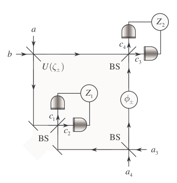
Figure 5.5: Schematic diagram of an eight-port homodyne detector.

Double homodyne, also called eight-port homodyne, detector is known for a long time for the joint determination of phase and amplitude of the field in microwave domain, and it was subsequently introduced in the optical domain [107].

A schematic diagram of the experimental setup is reported in Fig. 5.5. There are four input modes, which are denoted by $a$, $b$, $a_{3}$, and $a_{4}$, whereas the output modes, i.e. the modes that are detected, are denoted by $c_{k}$. There are four identical photodetectors whose quantum efficiency is given by $\eta$. The noise modes used to take into account inefficiency are denoted by $u_{k}$. The mixing among the modes is obtained through four balanced beam splitters: three of them (denoted by BS in Fig. 5.5) have real coupling $\zeta=\pi/4$, i.e. they do not impose any additional phase, whereas the fourth has evolution operator [see Eq. (1.67)] given by

$$U(\zeta_{\pm})=\exp\left\{\zeta_{\pm}a^{\dagger}b-\zeta_{\pm}^{*}ab^{\dagger}\right\}$$ (5.83a)

$$\zeta_{\pm}=\frac{\pi}{4}\,\exp\left\{i\left(\frac{\pi}{2}-\phi_{\pm}\right)\right\}\,,$$ (5.83b)

where $\phi_{\pm}=\pm\pi/2$ is the phase-shift imposed by a shifter (a quarter-wave plate) inserted in one arm. We consider $a$ and $b$ as signal modes. The mode $a_{4}$ is unexcited, whereas $a_{3}$ is placed in a highly excited coherent state $|z\rangle$ provided by an intense laser beam, and represents the local oscillator of the device. The detected photocurrents are $I_{k}=c^{{\dagger}}_{k}c_{k}$, which form the eight-port homodyne observables

$${Z}_{1}=\frac{I_{2}-I_{1}}{2\eta|z|}\,,\qquad{Z}_{2}=\frac{I_{3}-I_{4}}{2\eta|z|}\>.$$ (5.84)

The latter are derived by rescaling the difference photocurrent, each of them obtained in an homodyne scheme. In Eq. (5.84) $\eta$ denotes the quantum efficiency of the photodetectors whereas $|z|$ is the intensity of the local oscillator. In order to obtain ${Z}_{1}$ and ${Z}_{2}$ in terms of the input modes we first note that the input-output mode transformation is necessarily linear, as only passive components are involved in the detection scheme. Thus, we can write

$$c_{k}=\sum_{l=1}^{4}M_{kl}a_{l}\,,\qquad{{\boldsymbol{M}}}=\frac{1}{2}\left(\begin{array}[]{cccc}1&e^{i\theta_{\pm}}&-1&1\\ 1&e^{i\theta_{\pm}}&1&-1\\ -e^{-i\theta_{\pm}}&1&e^{i\phi_{\pm}}&e^{i\phi_{\pm}}\\ e^{-i\theta_{\pm}}&-1&e^{i\phi_{\pm}}&e^{i\phi_{\pm}}\end{array}\right)\>,$$ (5.89)

where $a_{1}=a$, $a_{2}=b$, $\theta_{\pm}=\frac{\pi}{2}-\phi_{\pm}$, and the transformation matrix ${\boldsymbol{M}}$ can be computed starting from the corresponding transformations for the beam splitters and the phase shifter. Eq. (5.89) together with the equivalent scheme for the inefficient detection leads to the following expression for the output modes, namely

$$c_{k}=\sqrt{\eta}\,\sum_{l=1}^{4}M_{kl}a_{l}+\sqrt{1-\eta}\>u_{k}\>.$$ (5.90)

Upon inserting Eqs. (5.90) in Eq. (5.84), and by considering the limit of highly excited local oscillator, we obtain the two photocurrents in terms of the input modes. If we set the phase shifter at $\phi_{+}$ and tune the fourth beam splitter accordingly we have

$${Z}_{1\eta+} =q_{a}+q_{b}+\sqrt{\frac{1-\eta}{\eta}}\left[q_{u_{1}}-q_{u_{2}}\right]+O(|z|^{-1})\,,$$ (5.91a)

$${Z}_{2\eta+} =p_{a}-p_{b}+\sqrt{\frac{1-\eta}{\eta}}\left[p_{u_{4}}-p_{u_{3}}\right]+O(|z|^{-1})\>,$$ (5.91b)

while if we choose $\phi_{-}$ we obtain

$${Z}_{1\eta-} =q_{a}-q_{b}+\sqrt{\frac{1-\eta}{\eta}}\left[q_{u_{1}}+q_{u_{2}}\right]+O(|z|^{-1})\,,$$ (5.92a)

$${Z}_{2\eta-} =p_{a}+p_{b}+\sqrt{\frac{1-\eta}{\eta}}\left[p_{u_{4}}+p_{u_{3}}\right]+O(|z|^{-1})\>,$$ (5.92b)

where $q_{k}$ and $p_{k}$ in Eqs. (5.92) denotes quadratures of the different modes for specific phases as following (we assume $\kappa_{1}=1$)

$$q\equiv x_{0}=\frac{1}{2}(a^{\dagger}+a)\,,\qquad p\equiv x_{\pi/2}=\frac{1}{2i}(a-a^{\dagger})\;.$$ (5.93)

Using Eq. (5.93) we may write the complex photocurrent ${Z}={Z}_{1}+i{Z}_{2}$ as follows

$${Z_{-}}=a-b^{{\dagger}}\,\quad\mbox{or}\quad{Z_{+}}=a+b^{{\dagger}}\>,$$ (5.94)

whereas, for non unit quantum efficiency, it becomes a Gaussian convolution of Eq. (5.94), as we will discuss in detail in Section 5.6.4.

It is worth noticing here that the mode transformation defined by Eq. (5.89) is distinctive for a canonical $4\times 4$-port linear coupler as defined in Refs. [108]. It has been rigorously shown [109] that a $N\times N$-port linear coupler can always be realized in terms of a number of beam splitters and phase-shifters. However, this implementation is, in general, not unique. The interest of eight-port homodyne scheme lies in the fact it provides the minimal scheme for realizing a $4\times 4$-multiport.

5.6.2 Heterodyne detector

Heterodyne detection scheme is known for a long time in radiophysics and it has been subsequently introduced in the domain of optics [110]. The term “heterodyne” comes from the fact that the involved modes are excited on different frequencies.

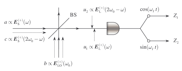
Figure 5.6: Schematic diagram of a heterodyne detection. Relevant modes are pointed out.

In Fig. 5.6 we show a schematic diagram of the detector. We denote by ${{\boldsymbol{E}}}_{\rm S}$ the signal field, whereas ${{\boldsymbol{E}}}_{\rm LO}$ describes the local oscillator. The field ${{\boldsymbol{E}}}_{\rm L}$ accounts for the losses due to inefficient photodetection. The input signal is excited in a single mode (say $a$) at the frequency $\omega$, as well as the local oscillator which is excited at a mode at the frequency $\omega_{0}$. This local oscillator mode is placed in a strong coherent state $|z\rangle$ by means of an intense laser beam. The beam splitter has a transmissivity given by $\tau$, whereas the photodetectors shows quantum efficiency $\eta$. The heterodyne output photocurrents are given by the real ${Z}_{1}$ and the imaginary ${Z}_{2}$ part of the complex photocurrent ${Z}$. The latter is obtained after the rescaling of the output photocurrent $I$, which is measured at the intermediate frequency $\omega_{I}=\omega-\omega_{0}$. By Fourier transform of Eq. (5.11) we have

$$I(\omega_{I})=\int_{\mathbb{R}}d\omega^{\prime}\;{{\boldsymbol{E}}}^{(-)}_{\rm O}(\omega^{\prime}+\omega_{I})\>{{\boldsymbol{E}}}^{(+)}_{\rm O}(\omega^{\prime})\;,$$ (5.95)

${{\boldsymbol{E}}}^{(\pm)}_{\rm O}$ being the positive and the negative part of the output field. In terms of the input fields Eq. (5.95) can be written as

$$I(\omega_{I})=\int_{\mathbb{R}}\!\!\!d\omega^{\prime}\Big{[}\sqrt{\eta\tau}{{\boldsymbol{E}}}^{(-)}_{\rm S}(\omega^{\prime}+\omega_{I})+\sqrt{\eta(1-\tau)}{{\boldsymbol{E}}}^{(-)}_{\rm LO}(\omega^{\prime}+\omega_{I})+\sqrt{1-\eta}{{\boldsymbol{E}}}^{(-)}_{\rm L}(\omega^{\prime}+\omega_{I})\Big{]}\\ \times\Big{[}\sqrt{\eta\tau}{{\boldsymbol{E}}}^{(+)}_{\rm S}(\omega^{\prime})+\sqrt{\eta(1-\tau)}{{\boldsymbol{E}}}^{(+)}_{\rm LO}(\omega^{\prime})+\sqrt{1-\eta}{{\boldsymbol{E}}}^{(+)}_{\rm L}(\omega^{\prime})\Big{]}\;.$$ (5.96)

Heterodyne photocurrent is obtained by the following rescaling

$${Z}=\lim_{\begin{subarray}{c}\tau\rightarrow 1\\ |z|\rightarrow\infty\end{subarray}}\frac{I(\omega_{I})}{|z|\eta\sqrt{\tau(1-\tau)}}\qquad\;\mbox{(with $|z|\sqrt{1-\tau}$ constant)}\;.$$ (5.97)

In practice, this definition corresponds to have a very intense local oscillator, which is allowed only for a little mixing with the signal mode [111]. In this limit only terms containing the local oscillator field ${\boldsymbol{E}}^{(\pm)}_{\rm LO}(\omega_{0})$ at the frequency $\omega_{0}$ can survive in Eq. (5.96), so that we have

$${Z}_{\eta-}={Z}_{1\eta-}+i{Z}_{2\eta-}\;,$$ (5.98)

where

$${Z}_{1\eta+} =q_{a}+q_{c}+\sqrt{\frac{1-\eta}{\eta}}\left[q_{u_{1}}-q_{u_{2}}\right]+O(|z|^{-1})\,,$$ (5.99a)

$${Z}_{2\eta+} =p_{a}-p_{c}+\sqrt{\frac{1-\eta}{\eta}}\left[p_{u_{1}}-p_{u_{2}}\right]+O(|z|^{-1})\>.$$ (5.99b)

In writing Eq. (5.99) we have substituted

$$c\leftarrow{{\boldsymbol{E}}}^{(+)}_{\rm S}(2\omega_{0}-\omega)\,,\qquad u_{1}\leftarrow{{\boldsymbol{E}}}^{(+)}_{\rm L}(\omega)\,,\qquad u_{2}\leftarrow{{\boldsymbol{E}}}^{(+)}_{\rm L}(2\omega_{0}-\omega)\,,$$ (5.100)

for the relevant modes involved. Since $u_{1}$ and $u_{2}$ are not excited, they play the role of noise modes accounting for the quantum efficiency of the photodetector. The expression (5.99) for the heterodyne photocurrents is thus equivalent to that of Eq. (5.91) for the eight-port homodyne scheme. The full equivalence of the two detection schemes has been thus proved. Also for heterodyne detection, a simple rearrangements of phase-shifts provides the measurement of the complex operators $Z_{+}$ instead of $Z_{-}$.

5.6.3 Six-port homodyne detector

A linear, symmetric three-port optical coupler is a straightforward generalization of the customary lossless symmetric beam splitter. The three input modes $a_{k}$, $k=1,2,3$, are combined to form 3 output modes $c_{k}$, $k=1,2,3$. In analogy to lossless beam splitters, which are described by unitary 2$\times$2 matrices [112], any lossless triple coupler is characterized by a unitary $3\times 3$ matrix [113]. For the symmetric case we have the form

$${{\boldsymbol{T}}}=\frac{1}{\sqrt{3}}\left(\begin{array}[]{ccc}1&1&1\\ 1&\xi&\xi^{*}\\ 1&\xi^{*}&\xi\end{array}\right)\;,$$ (5.104)

where $\xi=\exp\left\{i\frac{2}{3}\pi\right\}$ and each matrix element $T_{hk}$ represents the transmission amplitude from the $k$-th input port to the $h$-th output port, namely $c_{h}=\sum_{k=1}^{3}T_{hk}a_{k}$. Such devices have already been implemented in single-mode optical fiber technology and commercial triple coupler are available [114]. Any triple coupler can be also implemented by discrete optical components using symmetric beam splitters and phase shifters only [113]. As it has already mentioned in Section 5.6.1, this is due to the fact that that any unitary $m$-dimensional matrix can be factorized into a sequence of 2-dimensional transformations plus phase-shifts [109]. Moreover, this decomposition is not, in general, unique. In Fig. 5.7 we sketch a possible implementation of a triple coupler where the input modes are $a_{1}=a$, $a_{2}=b$, and $a_{3}$. Experimental realizations of triple couplers has been reported for both cases, the passive elements case and the optical fiber one [113, 115].

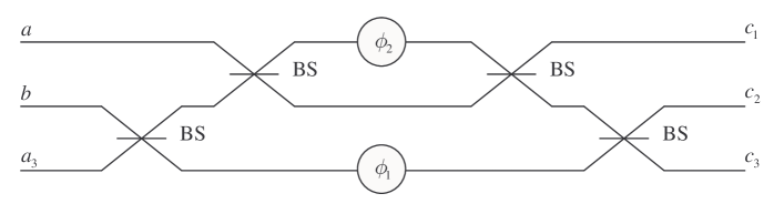
Figure 5.7: Realization of a triple coupler in terms of 50/50 beam splitters (BS) and phase shifters “$\phi$”. In order to obtain a symmetric coupler the following values has to be chosen: $\phi_{1}=\arccos(1/3)$ and $\phi_{2}=\phi_{1}/2$.

Let us now consider the measurement scheme of Fig. 5.8 [116]. The three input modes are mixed by a triple coupler and the resulting output modes are subsequently detected by three identical photodetectors. The measured photocurrents are proportional to $I_{n}$, $n=1,2,3$, given by

$$I_{n}=c^{{\dagger}}_{n}c_{n}=\frac{1}{3}\sum_{k,l=1}^{3}\exp\left\{i\theta_{n}(l-k)\right\}a_{k}^{{\dagger}}a_{l}\;,\qquad\theta_{n}=\frac{2\pi}{3}(n-1)\;,$$ (5.105)

where $a_{1}=a$ and $a_{2}=b$. After photodetection a Fourier transform (FT) on the photocurrents is performed

$${\cal I}_{s}\equiv{\rm FT}(I_{1},I_{2},I_{3})=\frac{1}{\sqrt{3}}\sum_{n=1}^{3}I_{n}\exp\left\{-i\theta_{n}(s-1)\right\}\;\qquad(s=1,2,3)\,.$$ (5.106)

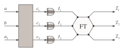
Figure 5.8: Outline of triple coupler homodyne detectors: the hexagonal box symbolizes the electronically performed Fourier transform (FT).

This procedure is a straightforward generalization of the customary two-mode balanced homodyning technique. In that case, in fact, the sum and the difference of the two output photocurrents are considered, which actually represent the Fourier transform in a two-dimensional space. By means of the identity

$$\delta_{3}(s-1)=\frac{1}{3}\sum_{n=1}^{3}\exp\left\{i\frac{2\pi}{3}n(s-1)\right\}\;,$$ (5.107)

for the periodic (modulus 3) Kronecker delta $\delta_{3}$, we obtain our final expressions for the Fourier transformed photocurrents:

$$\begin{array}[]{c}{\cal I}_{1}={\displaystyle\frac{1}{\sqrt{3}}}\left(a^{{\dagger}}a+b^{{\dagger}}b+a^{{\dagger}}_{3}a_{3}\right)\,,\\[8.61108pt] {\cal I}_{2}={\displaystyle\frac{1}{\sqrt{3}}}\left(a^{{\dagger}}b+b^{{\dagger}}a_{3}+a^{{\dagger}}_{3}a\right)\,,\qquad{\cal I}_{3}={\displaystyle\frac{1}{\sqrt{3}}}\left(a^{{\dagger}}a_{3}+b^{{\dagger}}a+a^{{\dagger}}_{3}b\right)\,.\end{array}$$ (5.108)

${\cal I}_{1}$ gives no relevant information as it is insensitive to the phase of the signal field, whereas ${\cal I}_{2}$ and ${\cal I}_{3}$ are hermitian conjugates of each other and contain the relevant information in their real and imaginary part. In the following let us assume $a$ and $b$ as the signal modes and $a_{3}$ fed by a highly excited coherent state $|z\rangle$ representing the local oscillator. For large $|z|$ the output photocurrents are intense enough to be easily detected. They can be combined to give the reduced photocurrents

$${Z}_{1+} =\sqrt{3}\,\frac{{\cal I}_{2}+{\cal I}_{3}}{2|z|}=q_{a}+q_{b}+O(|z|^{-1})\,,$$ (5.109a)

$${Z}_{2+} =\sqrt{3}\,\frac{{\cal I}_{3}-{\cal I}_{3}}{2i|z|}=p_{a}-p_{b}+O(|z|^{-1})\;,$$ (5.109b)

which we refer to as the triple homodyne photocurrents. Again, the complex photocurrent ${Z_{+}}={Z}_{1+}+i{Z}_{2+}$ has the form ${Z_{-}}=a+b^{{\dagger}}$, $a$ and $b$ being two modes of the field.

When accounting for the non unit quantum efficiency $\eta$ of the photodetectors the output modes are written as $c_{h}=\sqrt{\eta}\,\sum_{k=1}^{3}T_{hk}\,a_{k}+\sqrt{1-\eta}\>u_{h}$, $h=1,2,3$, so that the reduced photocurrents are now given by

$${Z}_{1\eta+} =\sqrt{3}\,\frac{{\cal I}_{2}+{\cal I}_{3}}{2\eta|z|}=q_{a}+q_{b}+\sqrt{\frac{1-\eta}{\eta}}\left[q_{u_{1}}+q_{u_{2}}\right]+O(|z|^{-1})\,,$$ (5.110a)

$${Z}_{2\eta+} =\sqrt{3}\,\frac{{\cal I}_{3}-{\cal I}_{2}}{2i\eta|z|}=p_{a}-p_{b}+\sqrt{\frac{1-\eta}{\eta}}\left[p_{u_{2}}-p_{u_{1}}\right]+O(|z|^{-1})\>.$$ (5.110b)

When, as it is the case, the modes $u_{k}$ are placed in the vacuum, the six-port photocurrents in Eq. (5.110) leads to the same statistics of the eight-port photocurrents in Eq. (5.91). Indeed, they describe different devices leading to the same amount of information on the signal modes. The measurements of $Z_{-}$ can also be achieved by six-port homodyne by a suitable choice of the phase-shifts among the modes.

5.6.4 Output statistics from a two-photocurrent device

Although the two pairs of single-mode quadratures $[q_{k},p_{k}]=i/2$, where $k=a,b$ are two modes of the field, do not commute, the sum and difference quadratures do, and therefore can be measured in a single experiment. Indeed, the three detection schemes analyzed in this Section provide the joint measurement of the operators $q_{a}+q_{b}$ and $p_{a}-p_{b}$, or $q_{a}-q_{b}$ and $p_{a}+p_{b}$. In turn, the two cases corresponds to the measurement of the real and the imaginary part of the complex photocurrents $Z_{\pm}=a\pm b^{\dagger}$ respectively. In both cases we have that $[Z_{\pm},Z_{\pm}^{\dagger}]=0=[\Re\hbox{e}[Z_{\pm}],\Im\hbox{m}[Z_{\pm}]]$, i.e. $Z_{\pm}$ are normal operators, and therefore the spectral theorem holds

$$Z_{\pm}=\int_{\mathbb{C}}d^{2}z\>z\>|z\rangle\rangle_{\pm}{}_{\pm}\langle\langle z|\>,$$

where $|z\rangle\rangle_{\pm}$ with $z\in{\mathbb{C}}$ are orthogonal eigenstates of $Z_{\pm}$, respectively.

Let us first consider $Z_{-}=a-b^{\dagger}$. Using the matrix notation introduced in Section 1.2 we have that

$$|z\rangle\rangle_{-}\equiv\frac{1}{\sqrt{\pi}}\>|D(z)\rangle\rangle=\frac{1}{\sqrt{\pi}}\>D(z)\otimes\mathbb{I}\,|\mathbbm{1}\rangle\rangle=\frac{1}{\sqrt{\pi}}\>\mathbb{I}\otimes D(-z^{*})|\mathbbm{1}\rangle\rangle\;,$$ (5.111)

where $D(z)$ is the displacement operator and $|\mathbbm{1}\rangle\rangle=\sum_{n}|n\rangle\otimes|n\rangle$. In fact

$$Z_{-}|z\rangle\rangle_{-} =\frac{1}{\sqrt{\pi}}\>D(z)D^{\dagger}(z)(a-b^{\dagger})D(z)|\mathbbm{1}\rangle\rangle$$

$$=\frac{1}{\sqrt{\pi}}\>D(z)(a+z-b^{\dagger})|\mathbbm{1}\rangle\rangle=\frac{1}{\sqrt{\pi}}\>D(z)\>z|\mathbbm{1}\rangle\rangle=z|z\rangle\rangle_{-}\>,$$ (5.112)

where we have used the fact that $a\otimes\mathbb{I}\,|\mathbbm{1}\rangle\rangle=\mathbb{I}\otimes b^{\dagger}|\mathbbm{1}\rangle\rangle$. Orthogonality of $|z\rangle\rangle_{-}$’s follows from that of displacement operators

$${}_{-}\langle\langle w|z\rangle\rangle_{-}=\frac{1}{\pi}\hbox{Tr}\left[D^{\dagger}(w)D(z)\right]=\delta^{(2)}(z-w)\;.$$ (5.113)

Notice that the eigenstates of the complex photocurrent $Z_{+}=a+b^{\dagger}$ may be analogously written as

$$|z\rangle\rangle_{+}=\frac{1}{\sqrt{\pi}}\>D(z)\otimes\mathbb{I}\,|\mathbb{J}\rangle\rangle\;,$$ (5.114)

where $[\mathbb{J}]_{pq}=(-)^{p}\>\delta_{pq}$, i.e. $|\mathbb{J}\rangle\rangle=\sum_{p}(-)^{p}\>|p\rangle\otimes|p\rangle$. If $R$ is the density matrix describing the quantum state of modes $a$ and $b$ the statistics of the measurement is described by the probability density

$$K_{\pm}(z)=\hbox{Tr}_{ab}\left[R\>E_{\pm}(z)\right]\,,$$

with $E_{\pm}(z)=|z\rangle\rangle_{\pm}{}_{\pm}\langle\langle z|$ denoting the overall POVM of the detector.

Let us now consider the effects of nonunit quantum efficiency. The measured photocurrents are given in Eqs. (5.91), (5.92), (5.99) or (5.110); using (5.9) the POVM $\Pi_{\eta}(z)$ is obtained upon tracing over the vacuum modes used to simulate losses: for either $\Pi_{\eta\pm}(z)$ we have

$$\Pi_{\eta}(z) = \int_{\mathbb{C}}\frac{d^{2}\gamma}{\pi^{2}}{}_{u_{1}u_{2}}\langle\langle 00|\exp\left\{\gamma(Z_{\eta}^{\dagger}-z^{*})-\gamma^{*}(Z_{\eta}-z)\right\}|00\rangle\rangle_{u_{1}u_{2}}$$ (5.115)

$$= \int_{\mathbb{C}}\frac{d^{2}\gamma}{\pi^{2}}\>\exp\left\{\gamma(Z_{+}-z^{*})-\gamma^{*}(Z_{-}-z)\right\}\>\exp\left\{-\frac{1-\eta}{\eta}|\gamma|^{2}\right\}$$

$$= \frac{\eta}{\pi(1-\eta)}\exp\left\{-\frac{\eta}{1-\eta}|Z-z|^{2}\right\}$$

$$= \int_{\mathbb{C}}\frac{d^{2}w}{\pi\Delta^{2}_{\eta}}\exp\left\{-\frac{|z-w|^{2}}{\Delta^{2}_{\eta}}\right\}\>E(z)\;,$$

where

$$\Delta^{2}_{\eta}=\frac{1-\eta}{\eta}\>.$$ (5.116)

The characteristic function of the POVM, for unit quantum efficiency, is given by

$$\chi[E_{-}(z)](\lambda_{1},\lambda_{2}) ={}_{-}\langle\langle z|D(\lambda_{1})\otimes D(\lambda_{2})|z\rangle\rangle_{-}$$

$$=\frac{1}{\pi}e^{\lambda_{1}z^{*}-\lambda_{1}^{*}z}\>\langle\langle\mathbbm{1}|D(\lambda_{1})\otimes D(\lambda_{2})|\mathbbm{1}\rangle\rangle$$

$$=\frac{1}{\pi}e^{\lambda_{1}z^{*}-\lambda_{1}^{*}z}\>\langle\langle\mathbbm{1}|D(\lambda_{1})D^{\scriptscriptstyle T}(\lambda_{2})\rangle\rangle$$

$$=\frac{1}{\pi}e^{\lambda_{1}z^{*}-\lambda_{1}^{*}z}\>\hbox{Tr}[D(\lambda_{1})D^{\scriptscriptstyle T}(\lambda_{2})]$$

$$=e^{\lambda_{1}z^{*}-\lambda_{1}^{*}z}\>\delta^{(2)}(\lambda_{1}-\lambda_{2}^{*})\>.$$ (5.117)

Analogously,

$$\chi[E_{+}(z)](\lambda_{1},\lambda_{2}) ={}_{+}\langle\langle z|D(\lambda_{1})\otimes D(\lambda_{2})|z\rangle\rangle_{+}$$

$$=\frac{1}{\pi}e^{\lambda_{1}z^{*}-\lambda_{1}^{*}z}\>\langle\langle\mathbb{J}|D(\lambda_{1})\otimes D(\lambda_{2})|\mathbb{J}\rangle\rangle$$

$$=\frac{1}{\pi}e^{\lambda_{1}z^{*}-\lambda_{1}^{*}z}\>\langle\langle\mathbb{J}|D(\lambda_{1})\>\mathbb{J}\>D^{\scriptscriptstyle T}(\lambda_{2})\rangle\rangle$$

$$=\frac{1}{\pi}e^{\lambda_{1}z^{*}-\lambda_{1}^{*}z}\>\hbox{Tr}[\boldsymbol{\Pi}\>D(\lambda_{1})\>\boldsymbol{\Pi}\>D^{\scriptscriptstyle T}(\lambda_{2})]$$

$$=e^{\lambda_{1}z^{*}-\lambda_{1}^{*}z}\>\delta^{(2)}(\lambda_{1}+\lambda_{2}^{*})\>,$$ (5.118)

where $\boldsymbol{\Pi}=\otimes_{k}(-)^{a^{\dagger}_{k}a_{k}}\equiv(-)^{\sum_{k}a^{\dagger}_{k}a_{k}}$ is the multimode parity operator. Using (5.117) and (5.118) we have

$$W[E_{\pm}(z)](\boldsymbol{X})=\frac{1}{\pi^{2}}\delta(x_{1}\pm x_{2}-x_{z})\delta(y_{1}\mp y_{2}-y_{z})\>,$$ (5.119)

where $z=x_{z}+iy_{z}$ and we used the Cartesian form of the Wigner function for the sake of simplicity.

For nonunit quantum efficiency $W[\Pi_{\eta\pm}](\boldsymbol{X})$ is given, according to Eq. (5.115), by a Gaussian convolution of $W[E_{\pm}(z)](\boldsymbol{X})$, i.e.

$$W[\Pi_{\eta\pm}](\boldsymbol{X})=\frac{1}{2\pi\Delta^{2}_{\eta}}\exp\left\{-\frac{(x_{1}\pm x_{2}-x_{z})^{2}}{2\Delta_{\eta}^{2}}-\frac{(y_{1}\mp y_{2}-y_{z})^{2}}{2\Delta_{\eta}^{2}}\right\}\>.$$ (5.120)

Let us now consider a situation in which $R$ is factorized, namely $R=\sigma\otimes\tau$. $\sigma$ is the state under investigation and $\tau$ a known reference state usually referred to as the probe of the detector (see Fig. 5.9). The statistics of the outcomes, for unit quantum efficiency, may be described as follows

$$K(z) =\hbox{Tr}_{ab}\left[\sigma\otimes\tau\>\Pi(z)\right]=\frac{1}{\pi}\hbox{Tr}_{a}\Big{[}\sigma\,\hbox{Tr}_{b}\big{[}\mathbb{I}\otimes\tau\>|D(z)\rangle\rangle\langle\langle D(z)|\big{]}\Big{]}$$

$$=\frac{1}{\pi}\hbox{Tr}_{a}\Big{[}\sigma\,\hbox{Tr}_{b}\big{[}|D(z)\tau^{\scriptscriptstyle T}\rangle\rangle\langle\langle D(z)|\big{]}\Big{]}=\hbox{Tr}_{a}\left[\sigma\>\Pi_{1}(z)\right]\,,\;$$ (5.121)

with

$$\Pi_{1}(z)=\frac{1}{\pi}D(z)\,\tau^{\scriptscriptstyle T}D^{\dagger}(z)\>,$$ (5.122)

which is the single mode POVM of the detector viewed as a measurement of the first mode probed by the second mode [117]. If $\tau=|0\rangle\langle 0|$ is the vacuum, then the POVM $\Pi_{1}(z)$ is the set of (nonorthogonal) projectors $|z\rangle\langle z|$ over coherent states, and setup measures the $Q$-function $Q(z)=\pi^{-1}\langle z|\sigma|z\rangle$ of the state $\sigma$. Notice that, as required for a POVM, $\Pi(z)$ is selfadjoint and normalized. The first property follows from the fact that $\tau$ itself is selfadjoint. In fact, $\tau^{\dagger}=\tau$ implies that $\tau^{\scriptscriptstyle T}=\tau^{*}$ and therefore $\Pi_{1}^{\dagger}(z)=\pi^{-1}D(z)\,\tau^{*}D^{\dagger}(z)=\pi^{-1}D(z)\,\tau^{\scriptscriptstyle T}D^{\dagger}(z)=\Pi_{1}(z)$. Normalization follows from completeness of the set of displacement operators, and in particular from Eq. (1.60b). The role of signal and probe may be exchanged, and the statistics can be written as follows

$$K(z) =\frac{1}{\pi}\hbox{Tr}_{b}\Big{[}\tau\,\hbox{Tr}_{a}\big{[}\sigma\otimes{\mathbb{I}}\>|D(z)\rangle\rangle\langle\langle D(z)|\big{]}\Big{]}$$

$$=\frac{1}{\pi}\hbox{Tr}_{b}\Big{[}\tau\,\hbox{Tr}_{a}\big{[}|\sigma D(z)\rangle\rangle\langle\langle D(z)|\big{]}\Big{]}=\hbox{Tr}_{b}\left[\tau\>\Pi_{2}(z)\right]\,,$$ (5.123)

where the POVM acting on the mode $b$ is given by

$$\Pi_{2}(z)=\frac{1}{\pi}D(-z^{*})\,\sigma^{\scriptscriptstyle T}D^{\dagger}(-z^{*})=\frac{1}{\pi}D^{\scriptscriptstyle T}(z)\,\sigma^{\scriptscriptstyle T}D^{*}(z)\>.$$ (5.124)

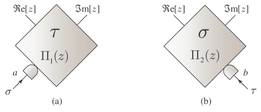
Figure 5.9: (a): measurement of the two-mode POVM $E(z)$ viewed as a single-mode measurement of the $\tau$-dependent POVM (5.122) on mode $a$; (b): the same for the POVM (5.124) on mode $b$.

The action of $\Pi_{1}(z)$ and $\Pi_{2}(z)$ is depicted in Fig. 5.9 (a) and (b) respectively. The Wigner functions of the POVMs $\Pi_{k}(z)$, $k=1,2$ are given by

$$W[\Pi_{1}(z)](\alpha) =\frac{1}{\pi}W[\tau^{\scriptscriptstyle T}](\alpha-z)=\frac{1}{\pi}W[\tau](\alpha^{*}-z^{*})\,,$$

$$W[\Pi_{2}(z)](\alpha) =\frac{1}{\pi}W[\sigma^{\scriptscriptstyle T}](\alpha+z^{*})=\frac{1}{\pi}W[\tau](\alpha^{*}+z)\,,$$ (5.125)

where we have used (1.143b) and the fact that transposition corresponds to mirror reflection in the phase space [see Eq. (3.7)]. For nonunit quantum efficiency the POVMs becomes Gaussian convolutions of the ideal POVM (with variance equal to $\Delta_{\eta}^{2}$). The Wigner functions modify accordingly.

Chapter 6 Nonlocality in continuous variable systems

In their famous paper of 1935 [118], Einstein, Podolsky and Rosen (EPR) introduced in quantum physics two strictly related concepts: entanglement and nonlocality, which afterward generated a longstanding debate on the completeness of quantum mechanics. These two concepts have become more and more important in the subsequent decades, as the recent progresses in quantum information science definitely demonstrated.

In Chapter 3 quantum entanglement for continuous variable (CV) systems has been extensively analyzed. We also pointed out that the concept of entanglement coincides with nonlocality only for the simple case of bipartite pure states. As soon as we deal with bipartite mixed states, entanglement can be found which do not show properties of nonlocality (while the converse instead is always true) [51].

This Chapter will be devoted to the issue of nonlocality for CV systems. First of all, we recall what the concept of nonlocality means. Usually two different notions are subsumed in it: (non-)locality and (non-)realism. A theory is said to be local if no action at distance, between two subsystems $A$ and $B$, is contemplated in it. Hence, quoting Einstein [120]:

“The real factual situation of the system $B$ is independent of what is done with the system $A$, which is spatially separated from the former.”

A realistic theory is a theory able to assign a definite counterpart to every element of reality and again following [118]:

“If, without in any way disturbing a system, we can predict with certainty (i.e., with probability equal one) the value of a physical quantity, then there exist an element of physical reality corresponding to this physical quantity.”

A theory which is not a local realistic one is simply incomplete, according to the spirit of EPR paper. Let us now apply this notions to a composite system of two distant particles, described by the so-called EPR wave function, i.e. the TWB wave function (1.115) in the limit of infinite squeezing. By measuring, say, the position of one particle the position of the other one can be predicted with certainty, as follows from the correlations between the two. If there is no action at distance, this prediction can be made without in any way disturbing the second particle. Hence an element of physical reality must be assigned to its position. On the other hand, the same argument apply to the measurement of momenta. However, quantum theory precludes the simultaneous assignment of position and momentum without uncertainty. So EPR conclude that quantum theory is not complete.

The debate about whether or not quantum mechanics is a local realistic theory remained in the realm of philosophy, rather of physics, for many years. The situation drastically changed when Bell proved that EPR point of view leads to algebraic predictions (the celebrated Bell’s inequalities) that are contradicted by quantum mechanics [72]. Bell formulated his inequalities in a dichotomized fashion, suitable for a discrete variable setting rather than for the original continuous variable one. In particular, Bell followed the simple and elegant formulation given by Bohm to the EPR gedanken experiment using spin-$\frac{1}{2}$ particles. More recently, however, the increasing importance of CV systems leads many authors to explore the nonlocality issue in its original setting, where dichotomic observables to test Bell’s inequalities are not uniquely determined. The attempts to translate Bell’s inequalities to CV clarified the fact that crucial in a nonlocality test is the existence of a set of dichotomized bounded observables used to perform the test itself, from which the so called Bell operator is derived. The more debated question has dealt with the nonlocality of the normalized version of the original EPR state, i.e. the TWB state of radiation. Nonlocality of the TWB was not clear for along time. Using the Wigner function approach, Bell argued that the original EPR state, and as a consequence the TWB too, does not exhibit nonlocality because its Wigner function is positive, and therefore represents a local hidden variable description [121]. More recently, Banaszek and Wodkiewicz [122] showed instead how to reveal nonlocality of the EPR state through the measurement of displaced parity operator. Furthermore a subsequent work of Chen et al. [123] showed that TWB’s violation of Bell’s inequalities may achieve the maximum value admitted by quantum mechanics upon a suitable choice of the measured observables. Indeed, the amount of violation crucially depends on the kind of Bell operator adopted in the analysis, ranging from no violation to maximal violation for the same (entangled) quantum state.

6.1 Nonlocality tests for continuous variables

In this Section we recall the inequalities imposed by local realism to the situations of our interest. Let us start by focusing our attention on a bipartite system. Let $m(\alpha)$ denotes a one-parameter family of single-system observable quantities with dichotomic spectrum. In the following $m(\alpha_{1})=\pm 1$ and $m(\alpha_{1}^{\prime})=\pm 1$ will denote the outcomes of the measurements on the first subsystem and, similarly, $m(\alpha_{2})=\pm 1$ and $m(\alpha_{2}^{\prime})=\pm 1$ for the second subsystem. The essential feature of this measurements is that they are local, dichotomic and bounded. The Bell’s combination

$$B_{2}\equiv m(\alpha_{1})\otimes m(\alpha_{2})+m(\alpha_{1})\otimes m(\alpha_{2}^{\prime})+m(\alpha_{1}^{\prime})\otimes m(\alpha_{2})-m(\alpha_{1}^{\prime})\otimes m(\alpha_{2}^{\prime})\,,$$ (6.1)

under the assumption of local realism, leads to the well known Bell-CHSH inequality [124]:

$${\cal B}_{2}\equiv\left|\langle B_{2}\rangle\right|=|E(\alpha_{1},\alpha_{2})+E(\alpha_{1},\alpha_{2}^{\prime})+E(\alpha_{1}^{\prime},\alpha_{2})-E(\alpha_{1}^{\prime},\alpha_{2}^{\prime})|\leq 2\;,$$ (6.2)

where $E(\alpha_{1},\alpha_{2})=\langle m(\alpha_{1})\otimes m(\alpha_{2})\rangle$ is the correlation function among the measurement results. If we describe the system quantum mechanically, then we have that

$$E(\alpha_{1},\alpha_{2})\equiv{\rm Tr}[R\,m(\alpha_{1})\otimes m(\alpha_{2})]\,,$$

$R$ being the density matrix of the system under investigation.

Bipartite entangled pure states violate (6.2) for a suitable choice of the observables $m(\alpha)$ and of the values of the parameters. Bipartite entangled mixed states may or may not violate (6.2). Systems which involves only two parties are the simplest setting where to study violation of local realism in quantum mechanics. A more complex scenario arises if multipartite systems are considered. Studying the peculiar quantum features of these systems is worthwhile in view of their relevance in the development of quantum communication technology, e.g. to manipulate and distribute information in a quantum communication network [46, 49]. Although the study of multipartite nonlocality has originated without the use of inequalities [70], an approach to derive Bell inequalities (so called Bell-Klyshko inequalities) has been developed [73, 74] also for these systems and applied to characterize their entanglement properties [75]. Being originally developed in the framework of discrete variables, these multiparty Bell inequalities have found application also in the characterization of continuous variable systems [125, 126]. Bell-Klyshko inequalities [73, 74, 75] provides a generalization of inequality (6.2) and are based on the following recursively defined Bell’s combination (operator)

$$B_{n}\equiv\frac{1}{2}\big{[}m(\alpha_{n})+m(\alpha_{n}^{\prime})\big{]}\otimes B_{n-1}+\frac{1}{2}\big{[}m(\alpha_{n})-m(\alpha_{n}^{\prime})\big{]}\otimes B^{\prime}_{n-1}\;,$$ (6.3)

where $B^{\prime}_{n}$ denotes the same expression as $B_{n}$ but with all the $\alpha_{n}$ and $\alpha_{n}^{\prime}$ exchanged, and $m(\alpha_{n})=\pm 1$, $m(\alpha_{n}^{\prime})=\pm 1$ denote the outcomes of the measurements on the $n$-th party of the system. Bell-Klyshko inequalities then read:

$${\cal B}_{n}\equiv|\langle B_{n}\rangle|\leq 2\,.$$ (6.4)

In the case of a three-partite system, local realism assumption imposes the following inequality from combination (6.3):

$${\cal B}_{3}\equiv|E(\alpha_{1},\alpha_{2},\alpha_{3}^{\prime})+E(\alpha_{1},\alpha_{2}^{\prime},\alpha_{3})+E(\alpha_{1}^{\prime},\alpha_{2},\alpha_{3})-E(\alpha_{1}^{\prime},\alpha_{2}^{\prime},\alpha_{3}^{\prime})|\leq 2\;,$$ (6.5)

where again $E(\alpha_{1},\alpha_{2},\alpha_{3})$ is the correlation function between the measurement results.

Quantum mechanical systems can violate inequalities (6.2) and(6.5) by a maximal amount given by, respectively, ${\cal B}_{2}\leq 2\sqrt{2}$ and ${\cal B}_{3}\leq 4$. In general ${\cal B}_{n}^{2}\leq 2^{n+1}$ holds (see, e.g., Ref. [75]).

We now briefly review three different strategies to reveal quantum nonlocality in the framework of continuous variables systems. These nonlocality tests are the basis for the analysis the will be performed in the remaining of the Chapter. In order to introduce the argument, recall that in the case of a discrete bipartite system, for example a spin-$\frac{1}{2}$ two particle system, the local dichotomic bounded observable usually taken into account is the spin of the particle in a fixed direction, say ${\bf d}$. Hence the correlation between two measurements performed over the two particles is $E({\bf d}_{1},{\bf d}_{2})=\langle{\bf d}_{1}\cdot\boldsymbol{\sigma}\otimes{\bf d}_{2}\cdot\boldsymbol{\sigma}\rangle$, where the operator $\boldsymbol{\sigma}=(\boldsymbol{\sigma}_{x},\boldsymbol{\sigma}_{y},\boldsymbol{\sigma}_{z})$ is decomposed on the Pauli matrices base and ${\bf d}_{1},{\bf d}_{2}$ are two unit vectors. The Bell operator is then given by the expression:

$$B_{2\boldsymbol{\sigma}}={\bf d}_{1}\cdot\boldsymbol{\sigma}\otimes{\bf d}_{2}\cdot\boldsymbol{\sigma}+{\bf d^{\prime}}_{1}\cdot\boldsymbol{\sigma}\otimes{\bf d}_{2}\cdot\boldsymbol{\sigma}+{\bf d}_{1}\cdot\boldsymbol{\sigma}\otimes{\bf d^{\prime}}_{2}\cdot\boldsymbol{\sigma}-{\bf d^{\prime}}_{1}\cdot\boldsymbol{\sigma}\otimes{\bf d^{\prime}}_{2}\cdot\boldsymbol{\sigma}\;.$$ (6.6)

Consider now a $n$-partite continuous variable system. Following the original argument by EPR it is quite natural attempting to reveal the nonlocality of this system trying to infer quadratures of one subsystem from those of the others. From now on, we will refer to this procedure as a homodyne nonlocality test ($H$), as quadrature measurements of radiation field are performed through homodyne detection. Here we identify the quadrature $x^{k}_{\vartheta}$, relative to mode $k$, according to the definition (1.13). As they are local but neither bounded nor dichotomic, quadrature observables are not immediately suitable to perform a nonlocality test based on Bell’s inequalities. The procedure to make them bounded and dichotomic is quite arbitrary and consist in the assignment of two domains $D_{+}$ and $D_{-}$ to each observable [127]. When the result of a quadrature measurement falls in the domain $D_{\pm}$ the value $\pm 1$ is associated to it. Usually the choice $D_{\pm}=\mathbb{R}^{\pm}$ is considered, though a choice suitable to the system under investigation may be preferable. Considering a bipartite system we can introduce the following quantities

$$P_{++}(x_{\vartheta}^{1},x_{\varphi}^{2})=\int_{D_{+}}dx_{\vartheta}^{1}\int_{D_{+}}dx_{\varphi}^{2}P(x_{\vartheta}^{1},x_{\varphi}^{2})$$ (6.7a)

$$P_{+-}(x_{\vartheta}^{1},x_{\varphi}^{2})=\int_{D_{+}}dx_{\vartheta}^{1}\int_{D_{-}}dx_{\varphi}^{2}P(x_{\vartheta}^{1},x_{\varphi}^{2})$$ (6.7b)

$$P_{-+}(x_{\vartheta}^{1},x_{\varphi}^{2})=\int_{D_{-}}dx_{\vartheta}^{1}\int_{D_{+}}dx_{\varphi}^{2}P(x_{\vartheta}^{1},x_{\varphi}^{2})$$ (6.7c)

$$P_{--}(x_{\vartheta}^{1},x_{\varphi}^{2})=\int_{D_{-}}dx_{\vartheta}^{1}\int_{D_{-}}dx_{\varphi}^{2}P(x_{\vartheta}^{1},x_{\varphi}^{2})\;$$ (6.7d)

where $P(x_{\vartheta}^{1},x_{\varphi}^{2})$ is the joint probability distribution of the quadratures $x_{\vartheta}^{1}$ and $x_{\varphi}^{2}$. We can now identify the homodyne correlation function $E_{\scriptscriptstyle H}(\vartheta,\varphi)$ as

$$E_{\scriptscriptstyle H}(\vartheta,\varphi)=P_{++}(x_{\vartheta}^{1},x_{\varphi}^{2})+P_{--}(x_{\vartheta}^{1},x_{\varphi}^{2})-P_{+-}(x_{\vartheta}^{1},x_{\varphi}^{2})-P_{-+}(x_{\vartheta}^{1},x_{\varphi}^{2})\;,$$ (6.8)

which can be straightforwardly used to construct the Bell combination ${\cal B}_{2{\scriptscriptstyle H}}$ of Eq. (6.2) and to perform the nonlocality test. The main problem of pursuing such a nonlocality test is that it is not suitable in case of systems described by a positive Wigner function, as the TWB state of radiation. Indeed, a positive Wigner function can be interpreted as a hidden phase-space probability distribution, preventing violation of Bell-CHSH inequality unless the measured observables have an unbounded Wigner representation, which is not the case of the dichotomized quadrature measurement described above. In fact $P(x_{\vartheta}^{1},x_{\varphi}^{2})$ can be determined as a marginal distribution from the Wigner function. From Eqs. (6.7) and (6.8) one has

$$E_{\scriptscriptstyle H}(\vartheta,\varphi)=\int_{\mathbb{R}^{4}}dx_{\vartheta}^{1}\,dx_{\varphi}^{2}\,dx_{\vartheta+\frac{\pi}{2}}^{1}\,dx_{\varphi+\frac{\pi}{2}}^{2}\,{\rm sgn}\big{[}x_{\vartheta}^{1}\,x_{\varphi}^{2}\big{]}W(x_{\vartheta}^{1},x_{\vartheta+\frac{\pi}{2}}^{1},\,x_{\varphi}^{2},x_{\varphi+\frac{\pi}{2}}^{2})\;,$$ (6.9)

where the integration is performed over the whole phase-space and without loss of generality we have considered $D_{\pm}={\mathbb{R}}^{\pm}$. Eq. (6.9) itself is indeed a local hidden variable description of the correlation function, hence obeying inequality (6.2).

In order to overcome this obstacle different strategies have been considered by many authors, based essentially on parity measurements. Banaszek and Wodkiewicz [122] have demonstrated the nonlocality of the TWB considering as local observable on subsystem $k$ the parity operator on the state displaced by $\alpha_{k}$ (hence we will refer to this procedure as a displaced parity ($DP$) test), which is dichotomic and bounded:

$$\Pi(\boldsymbol{\alpha})=\bigotimes_{k=1}^{n}D_{k}(\alpha_{k})(-1)^{n_{k}}D_{k}^{\dagger}(\alpha_{k}).$$ (6.10)

In the above formula, $\boldsymbol{\alpha}=(\alpha_{1},\ldots,\alpha_{n})$, while $n_{k}=a_{k}^{\dagger}a_{k}$ and $D_{k}(\alpha_{k})$ denote the number operator and the phase space displacement operator for the subsystem $k$, respectively. Hence the correlation function reads:

$$E_{{\scriptscriptstyle DP}}(\boldsymbol{\alpha})=\langle\Pi(\boldsymbol{\alpha})\rangle,$$ (6.11)

from which Bell’s combinations ${\cal B}_{2{\scriptscriptstyle DP}}$ in Eq. (6.2) and ${\cal B}_{3{\scriptscriptstyle DP}}$ in Eq. (6.5) can be easily reconstructed in the cases $n=2,3$. The reason why this procedure would be able to reveal nonlocality also in case of quantum states characterized by a positive Wigner function is clear using the following relation [see Eq. (1.135)]:

$$W(\boldsymbol{\alpha})=\left(\frac{2}{\pi}\right)^{n}\langle\Pi(\boldsymbol{\alpha})\rangle\>.$$ (6.12)

Indeed, the analog of Eq. (6.9) is:

$$E_{{\scriptscriptstyle DP}}(\boldsymbol{\alpha})=\int_{\mathbb{C}^{n}}d^{2n}\boldsymbol{\lambda}\left(\frac{2}{\pi}\right)^{n}W(\boldsymbol{\alpha})\,\delta^{(2n)}(\boldsymbol{\alpha}-\boldsymbol{\lambda})\;.$$ (6.13)

Since the Dirac-$\delta$ distribution is unbounded, then Ineqs. (6.2) and (6.5) are no more necessarily valid for ${\cal B}_{2{\scriptscriptstyle DP}}$ and ${\cal B}_{3{\scriptscriptstyle DP}}$.

Another strategy, developed by Chen et al. [123], shares a similar behavior as the one described above, allowing to reveal nonlocality for quantum states with positive Wigner function. This type of nonlocality test will be referred to as Pseudospin ($PS$) nonlocality test. It can be seen as a generalization to CV systems of the strategy introduced by Gisin and Peres for the case of discrete variable systems [53], hence, for the case of a pure bipartite system, it is equivalent to an entanglement test [129]. Let us consider the following set of operators, known as pseudospins in view of their commutation relations, ${\bf s}_{k}=(s^{k}_{x},s^{k}_{y},s^{k}_{z})$ acting on the $k$-th subsystem

$$s^{k}_{z}=\sum_{n=0}^{\infty}\big{(}|2n+1\rangle_{k}{}_{k}\langle 2n+1|-|2n\rangle_{k}{}_{k}\langle 2n|\big{)}\,,$$ (6.14a)

$$s^{k}_{x}\pm is^{k}_{y}=2s^{k}_{\pm}\,,$$ (6.14b)

$${\bf d}_{k}{\bf s}_{k}=\cos\vartheta_{k}\,s^{k}_{z}+\sin\vartheta_{k}\,(e^{i\varphi_{k}}s^{k}_{-}+e^{-i\varphi_{k}}s^{k}_{+})\,,$$ (6.14c)

where $s^{k}_{-}=\sum_{n}|2n\rangle_{k}{}_{k}\langle 2n+1|=(s^{k}_{+})^{\dagger}$ and ${\bf d}_{k}$ is a unit vector associated to the angles $\vartheta_{k}$ and $\varphi_{k}$. In analogy to the spin-$\frac{1}{2}$ system mentioned above and defining the vector ${\bf d}=({\bf d}_{1},\ldots,{\bf d}_{n})$ the correlation function is simply given by:

$$E_{{\scriptscriptstyle PS}}({\bf d})=\langle\otimes_{k=1}^{n}{\bf d}_{k}{\bf s}_{k}\rangle\;,$$ (6.15)

from which the Bell combinations ${\cal B}_{2{\scriptscriptstyle PS}}$ and ${\cal B}_{3{\scriptscriptstyle PS}}$ are evaluated. Also different representations of the spin-$\frac{1}{2}$ algebra have been discussed in the recent literature [130, 131, 132]. In particular in Ref. [132] it has been pointed out that different representations lead to different expectation values of the Bell operators. Hence, the violation of Bell inequality for CV systems turns out to depend, besides to orientational parameters, also to configurational ones. In the following Sections we will also consider the pseudospin operators ${\bf\Pi}_{k}=(\Pi_{x}^{k},\Pi_{y}^{k},\Pi_{z}^{k})$ taken into account in Ref. [132], which have the following Wigner representation (for $\kappa_{1}=2^{-1/2}$):

$$\begin{array}[]{c}W[\Pi_{x}^{k}](\alpha_{k})={\rm sgn}\big{[}\Re\mbox{e}[\alpha_{k}]\big{]}\,,\qquad W[\Pi_{y}^{k}](\alpha_{k})=-\delta^{(2)}\big{(}\Re\mbox{e}[\alpha_{k}]\big{)}~{}{\cal P}{\displaystyle\frac{1}{\Im\mbox{m}[\alpha_{k}]}}\,,\\[8.61108pt] W[\Pi_{z}^{k}](\alpha_{k})=-\pi\delta^{(2)}(\alpha_{k})\,,\end{array}$$ (6.16)

where ${\cal P}$ stands for the “principal value”. The correlation function obtained using operators ${\bf\Pi}_{k}$ will be indicated as ${\cal E}_{{\scriptscriptstyle PS}}({\bf d})=\langle\otimes_{k=1}^{n}{\bf d}_{k}{\bf\Pi}_{k}\rangle$.

6.2 Two-mode nonlocality

In this Section we will analyze the nonlocality properties of two-mode states. First we concentrate on the TWB state of radiation, then we will consider non-Gaussian states and apply to them all the strategies introduced in the preceding section.

6.2.1 Twin-beam state

As already mentioned, the more debated question concerning nonlocality in continuous variable systems involved the TWB state, due to its importance both from an applicative point of view and from a fundamental perspective, as it is a normalized version of the original EPR state. Since it is not suitable for homodyne test, the TWB nonlocality will be investigated exploiting the $DP$ and $PS$ tests.

Displaced parity test

Let us follow Ref. [122]. Using Eq. (2.41) for the Wigner function of the TWB and Eq. (6.12), it is immediate to evaluate the correlation function $E_{{\scriptscriptstyle DP}}(\alpha_{1},\alpha_{2})$ of Eq. (6.11). In Ref. [122] the following parameterization has been considered to construct the Bell combination ${\cal B}_{2{\scriptscriptstyle DP}}$

$$\alpha_{1}=\alpha_{2}=0\,,\qquad\alpha_{1}^{\prime}=-\alpha_{2}^{\prime}=\sqrt{{\cal J}}\;.$$ (6.17)

It follows that

$${\cal B}_{2{\scriptscriptstyle DP}}=1+2\exp\{-2{\cal J}\cosh(2r)\}-\exp\{-4{\cal J}e^{2r}\}\;.$$ (6.18)

Figure 6.1: (a) Plot of the combination ${\cal B}_{2{\scriptscriptstyle DP}}$ defined in Eq. (6.18) and (b) according to the parametrization given by Eq. (6.20). Only values exceeding the bound imposed by local theories are shown.

As depicted in Fig. 6.1(a), ${\cal B}_{2{\scriptscriptstyle DP}}$ in (6.18) violates the upper bound imposed by local theories. For increasing $r$, the violation of the Bell’s inequality is observed for smaller ${\cal J}$. Therefore an asymptotic analysis for large $r$ and ${\cal J}\ll 1$ may be performed. Then a straightforward calculation shows that the maximum value of ${\cal B}_{2}$ (for this particular selection of coherent displacements) is obtained for

$${\cal J}e^{2r}=\frac{1}{3}\ln 2,$$ (6.19)

corresponding to ${\cal B}_{2{\scriptscriptstyle DP}}=1+3\cdot 2^{-4/3}\approx 2.19$. Thus, in the limit $r\rightarrow\infty$, when the original EPR state is recovered, a significant violation of Bell’s inequality takes place. Notice that in order to observe the nonlocality of the EPR state, very small displacements have to be applied, decreasing as ${\cal J}\propto e^{-2r}$. As pointed out in Ref. [122] the results above have been obtained without any serious attempt to find the maximum violation. For this purpose one should consider a general quadruplet of displacements. An analysis to obtain the maximum violation of Bell inequalities within this formalism is performed in [133]. Choosing

$$\alpha_{1}=-\alpha_{2}=i\sqrt{{\cal J}}\alpha_{1}^{\prime}=-\alpha_{2}^{\prime}=-3i\sqrt{{\cal J}}$$ (6.20)

an asymptotic violation of ${\cal B}_{2}\simeq 2.32$ can be obtained (see Fig. 6.1(b)). This shows that the EPR state does not maximally violate Bell’s inequalities in a DP test. The reason for this has been addressed in Ref. [129], and it is attributed to the fact that the displaced parity operator does not completely flip the parity of the entangled quantities characterizing the TWB (i.e., the number states).

Pseudospin test

Let us now focus on the “pseudospin nonlocality test”. Considering a TWB state, it is known that the correlation function (6.15) has the following expression (setting to zero the azimuthal angles) [123]:

$$E_{{\scriptscriptstyle PS}}(\vartheta_{1},\vartheta_{2})=\cos\vartheta_{1}\cos\vartheta_{2}+f_{\hbox{\tiny TWB}}\sin\vartheta_{1}\sin\vartheta_{2}\>,$$ (6.21)

where $f_{\hbox{\tiny TWB}}=\tanh(2r)$. Choosing $\vartheta_{1}=0$, $\vartheta_{1}^{\prime}=\pi/2$ and $\vartheta_{2}=-\vartheta_{2}^{\prime}$, we have

$${\cal B}_{2}=2(\cos\vartheta_{2}+f_{\hbox{\tiny TWB}}\sin\vartheta_{2})\;,$$ (6.22)

and, for this specific setting, the maximum of ${\cal B}_{2}$ is

$${\cal B}_{2}=2\sqrt{1+f_{\hbox{\tiny TWB}}}\,.$$ (6.23)

It turns out that the TWB state violates the Bell’s inequality (6.2) for every $r\neq 0$. The violation increases monotonically to the maximum value of $2\sqrt{2}$ as the function $f_{\hbox{\tiny TWB}}\to 1$, i.e., as the squeezing parameter $r$ increases. This indicates that the EPR state maximally violate Bell’s inequality. Furthermore, $f_{\hbox{\tiny TWB}}$ may be regarded as a quantitative measure of quantum nonlocality.

In Ref. [132] different representations of ${\rm SU}(2)$ algebra have been considered to exploit nonlocality of the TWB. In particular using the operators given in Eq. (6.16) one can show that the correlation ${\cal E}_{{\scriptscriptstyle PS}}$ is still given by Eq. (6.21), where now the function $f_{\hbox{\tiny TWB}}$ is substituted by

$$f^{\prime}_{\hbox{\tiny TWB}}=\frac{2}{\pi}\arctan[\sinh(2r)]\;.$$ (6.24)

Therefore, the behavior of the Bell combination ${\cal B}_{2}$ is the same as above, but for any squeezing parameter $r$ it gives a lower violation of local realism if compared to Eq. (6.23). In general, it is possible to demonstrate that the configurational parameterization given by Eq. (6.14) leads to maximal violation for all values of $r$. Finally, we mention that besides the representations of ${\rm SU}(2)$ given by Eq. (6.14) and Eq. (6.16), different ones may be found for which the Bell combination ${\cal B}_{2}$ is not even a monotonic function of $r$, i.e. is not a monotonic function of the entanglement.

6.2.2 Non-Gaussian states

As already pointed out in Section 5.4, it is expected that non-Gaussian states are characterize by a larger nonlocality. Let us now exploit this possibility using the non-Gaussian states introduced in Section 5.4. Since the Wigner function of IPS and TWBA states is non-positive, all the nonlocality tests introduced will be considered.

Displaced parity test

In addressing nonlocality of IPS state, we will consider both the parameterizations (6.17) and (6.20). We denote $B({\cal J})\equiv\mathcal{B}_{2{\scriptscriptstyle DP}}$ for parameter Eq. (6.17), and $C({\cal J})\equiv\mathcal{B}_{2{\scriptscriptstyle DP}}$ for parameter Eq. (6.20). As for a TWB, the violation of the Bell’s inequality is observed for small $r$ [122]. For the rest of the section, we will refer to $B({\cal J})$ as $B^{\hbox{\tiny(TWB)}}({\cal J})$ when it is evaluated for a TWB (5.28), and as $B^{\hbox{\tiny(IPS)}}({\cal J})$ when we consider the IPS state (5.48).

Figure 6.2: Plot of $B({\cal J})$ for ${\cal J}=10^{-2}$. The dashed line is $B^{\hbox{\tiny(TWB)}}({\cal J})$, while the solid lines are $B^{\hbox{\tiny(IPS)}}({\cal J})$ for different values of $\tau_{\rm eff}$ (see the text): from top to bottom $\tau_{\rm eff}=0.999,0.99$ and $0.9$. When $\tau_{\rm eff}=0.999$, the maximum of $B^{\hbox{\tiny(IPS)}}({\cal J})$ is $2.23$. The plot on the right is a magnification of the region $0\leq r\leq 0.11$ of the upper one. Notice that for small $r$ there is always a region where $B^{\hbox{\tiny(TWB)}}({\cal J})<B^{\hbox{\tiny(IPS)}}({\cal J})$.

We plot $B^{\hbox{\tiny(TWB)}}({\cal J})$ and $B^{\hbox{\tiny(IPS)}}({\cal J})$ in the Figs. 6.2 and 6.3 for different values of the effective transmissivity $\tau_{\rm eff}$ and of the parameter $J$: for not too big values of the squeezing parameter $r$, one has that $2<B^{\hbox{\tiny(TWB)}}({\cal J})<B^{\hbox{\tiny(IPS)}}({\cal J})$. Moreover, when $\tau_{\rm eff}$ approaches unit, i.e. when at most one photon is subtracted from each mode, the maximum of $B{\hbox{\tiny(IPS)}}$ is always greater than the one obtained using a TWB. A numerical analysis shows that in the limit $\tau_{\rm eff}\to 1$ the maximum is $2.27$, that is greater than the value $2.19$ obtained for a TWB [122]. The limit $\tau_{\rm eff}\to 1$ corresponds to the case of one single photon subtracted from each mode [93, 94]. Notice that increasing ${\cal J}$ reduces the interval of the values of $r$ for which one has the violation. For large $r$ the best result is thus obtained with the TWB since, as the energy grows, more photons are subtracted from the initial state [92]. Since the relevant parameter for violation of Bell inequalities is $\tau_{\rm eff}$, we have, from Eq. (5.44), that the IPS state is nonlocal also for low quantum efficiency of the IPS detector.

Figure 6.3: Plots of $B({\cal J})$ as a function of the squeezing parameter $r$ for two different values of $J$: (a) ${\cal J}=5\cdot 10^{-2}$ and (b) ${\cal J}=10^{-1}$. In all the plots the dashed line is $B^{\hbox{\tiny(TWB)}}({\cal J})$, while the solid lines are $B^{\hbox{\tiny(IPS)}}({\cal J})$ for different values of $\tau_{\rm eff}$ (see the text): from top to bottom $\tau_{\rm eff}=0.999,0.9,0.8,0.7$ and $0.5$. Notice that there is always a region for small $r$ where $B^{\hbox{\tiny(TWB)}}({\cal J})<B^{\hbox{\tiny(IPS)}}({\cal J})$. When $\tau_{\rm eff}=0.999$ the maximum of $B^{\hbox{\tiny(IPS)}}({\cal J})$ is always greater than the one of $B^{\hbox{\tiny(TWB)}}({\cal J})$.

The same conclusions holds when we consider the parametrization of Eq. (6.20). In Fig. 6.4 we plot $C^{\hbox{\tiny(TWB)}}({\cal J})$ and $C^{\hbox{\tiny(IPS)}}({\cal J})$, i.e. $C({\cal J})$ evaluated for the TWB and the IPS state, respectively. The behavior is similar to that of $B({\cal J})$, the maximum violation being now $C^{\hbox{\tiny(IPS)}}({\cal J})=2.43$ for $\tau_{\rm eff}=0.9999$ and ${\cal J}=1.6\cdot 10^{-3}$. Finally, notice that the maximum violation using IPS states is achieved (for both parameterizations) when $\tau_{\rm eff}$ approaches unit and for values of $r$ smaller than for TWB.

Figure 6.4: Plots of $C({\cal J})$ as a function of the squeezing parameter $r$ for ${\cal J}=1.6\cdot 10^{-3}$. In all the plots the dashed line is $C^{\hbox{\tiny(TWB)}}({\cal J})$, while the solid lines are $C^{\hbox{\tiny(IPS)}}({\cal J})$ for different values of $\tau_{\rm eff}$ (see the text): from top to bottom $\tau_{\rm eff}=0.9999,0.999,0.99$ and $0.9$. When $\tau_{\rm eff}=0.9999$ the maximum of $C^{\hbox{\tiny(IPS)}}({\cal J})$ is $2.43$.

Concerning the TWBA (5.4.2), let us consider the case of large $N_{2}$ and small $N_{3}$, say $N_{3}=10^{-2}(N_{2})^{-1}$. As in the analysis of the entanglement properties of the tripartite state $|T\rangle$, the phase coefficients $\phi_{2}$ and $\phi_{3}$ play no role in the characterization of nonlocality. Using the parametrization $\alpha_{1}=\frac{1}{2}\alpha_{2}=\frac{1}{3}\alpha_{1}^{\prime}=i\sqrt{{\cal J}}$ and $\alpha_{2}^{\prime}=0$, an enhancement of the violation of Bell’s inequality can be observed with respect to the TWB. Indeed the asymptotic violation turns out to be of ${\cal B}_{2{\scriptscriptstyle DP}}=2.41$. It can be found, for large $N_{2}$, when ${\cal J}N_{2}=0.042$ (see Fig. 6.5).

Figure 6.5: Bell combination obtained choosing optimized displacement parameters for TWBA state (5.4.2) (see text for details). Only values violating inequality (6.2) are shown.

Although the IPS and the TWBA states allow for an enhancement of nonlocality with respect to the usual TWB state, they never reach the maximum violation admitted by quantum mechanics. As already pointed out the reason for this can be attributed to the fact that the displaced parity operator does not completely flip the parity of the entangled quantities characterizing the three states above (i.e. the number states). However, the maximum violation of the Bell’s inequality in the contest of a DP test could be achieved if the following state $|\hbox{ECS}\rangle$ (entangled coherent state) [134] could be produced experimentally

$$|{\rm ECS}\rangle={\cal N}(|\gamma\rangle|-\gamma\rangle-|-\gamma\rangle|\gamma\rangle)\;,$$ (6.25)

where ${\cal N}$ is a normalization factor and $|\gamma\rangle$ is a coherent state with $\gamma\neq 0$. Its Wigner function read as follows:

$$W_{\hbox{\tiny ECS}}(\alpha,\beta)=4{\cal N}^{2}\Big{\{}\exp\{-2|\alpha-\gamma|^{2}-2|\beta+\gamma|^{2}\}+\exp\{-2|\alpha+\gamma|^{2}-2|\beta-\gamma|^{2}\}\\ -\exp\{-2(\alpha-\gamma)(\alpha^{*}+\gamma)-2(\beta+\gamma)(\beta^{*}-\gamma)-4\gamma^{2}\}\\ -\exp\{-2(\alpha^{*}-\gamma)(\alpha+\gamma)-2(\beta^{*}+\gamma)(\beta-\gamma)-4\gamma^{2}\}\Big{\}}\;,$$ (6.26)

where $\gamma$ is assumed to be real for simplicity. Notice that the ECS state may be represented in the $2\times 2$-Hilbert space as

$$|{\rm ECS}\rangle=\frac{1}{\sqrt{2}}(|e\rangle|d\rangle-|d\rangle|e\rangle),$$ (6.27)

where $|e\rangle={\cal N_{+}}(|\gamma\rangle+|-\gamma\rangle)$ and $|d\rangle={\cal N_{-}}(|\gamma\rangle-|-\gamma\rangle)$ are even and odd states with normalization factors ${\cal N_{+}}$ and ${\cal N_{-}}$. Note that these states form an orthogonal basis, regardless of the value of $\gamma$, which span the two-dimensional Hilbert space. For this state the maximum violation can be achieved due to the fact the displaced parity operators act like an ideal rotation on the even and odd microscopic states $|e\rangle$ and $|d\rangle$ in which the ECS state may be decomposed [see Eq. (6.27)]. As a consequence the parity of $|e\rangle$ and $|d\rangle$, which are the orthogonal entangled elements in the entangled coherent state, can be perfectly flipped by the displacement operator (for $\gamma\rightarrow\infty$), allowing for the maximum violation of Bell’s inequality [129].

Pseudospin test

Figure 6.6: Plots of ${\cal B}_{PS}$: the dashed line refers to the TWB, whereas the solid lines refer to the IPS with, from top to bottom, $\tau_{\rm eff}=0.9999,0.99,0.9$, and $0.8$.

Now we investigate the nonlocality of the IPS state by means of the pseudospin test considering the pseudospin operators given in Eqs. (6.16). If we set to zero the azimuthal angle, the correlation function (6.15) reads

$$E_{{\scriptscriptstyle PS}}^{\hbox{\tiny(IPS)}}(\vartheta_{1},\vartheta_{2})=\frac{1}{p_{11}(r,\tau_{\rm eff})}\sum_{k=1}^{4}{\cal C}_{k}\,\big{[}\cos\vartheta_{1}\cos\vartheta_{2}+f_{\hbox{\tiny IPS}}\,\sin\vartheta_{a}\sin\vartheta_{b}\big{]}\,,$$ (6.28)

where we defined

$$f_{\hbox{\tiny IPS}}=\frac{8}{\pi{\cal A}_{k}}\,\arctan\left(\frac{2B\tau_{\rm eff}+h_{k}}{\sqrt{{\cal A}_{k}}}\right)\,,$$

with

$${\cal A}_{k}=(b-f_{k})(b-g_{k})-(2B\tau_{\rm eff}+h_{k})^{2}\,,$$

and all the quantities appearing in Eq. (6.28) have been defined in Section 5.4.1.

In Fig. 6.6 we plot ${\cal B}_{{\scriptscriptstyle PS}}$ for the TWB and IPS; we set $\vartheta_{1}=0$, $\vartheta^{\prime}_{1}=\pi/2$, and $\vartheta_{2}=-\vartheta^{\prime}_{2}=\pi/4$. As usual the IPS leads to better results for small values of $r$. Whereas ${\cal B}_{{\scriptscriptstyle PS}}^{\hbox{\tiny(TWB)}}\to 2\sqrt{2}$ as $r\to\infty$, ${\cal B}_{{\scriptscriptstyle PS}}^{\hbox{\tiny(IPS)}}$ has a maximum and, then, falls below the threshold $2$ as $r$ increases. It is interesting to note that there is a region of small values of $r$ for which ${\cal B}_{{\scriptscriptstyle PS}}^{\hbox{\tiny(TWB)}}\leq 2<{\cal B}_{{\scriptscriptstyle PS}}^{\hbox{\tiny(IPS)}}$, i.e. the IPS process can increases the nonlocal properties of a TWB which does not violates the Bell’s inequality for the pseudospin test, in such a way that the resulting state violates it. Note that the maximal of violation for the IPS occur for a range of values $r$ experimentally achievable.

Concerning the TWBA state, a straightforward calculation shows that an expression identical in form to Eq. (6.21), where the following function $f_{\hbox{\tiny TWBA}}$ can be identified:

$$f_{\hbox{\tiny TWBA}}=2\,{\sqrt{\frac{N_{2}}{1+N_{1}}}}\,\frac{\left(1+N_{3}\,\eta\right)}{N_{3}\,\left(1+N_{1}\right)\,\eta}\\ \times\sum_{k,p=0}^{\infty}\frac{\left(2\,k+p\right)!}{\left(2\,k\right)!\,p!}\,{\sqrt{\frac{2\,k+p+1}{2\,k+1}}}\,\left(1-{\left(1-\eta\right)}^{p}\right){\left(\frac{N_{3}}{1+N_{1}}\right)}^{p}\,{\left(\frac{N_{2}}{1+N_{1}}\right)}^{2\,k}\>.$$ (6.29)

In order to compare the violations in the case of the TWB and the TWBA, let us fix as in the previous subsection a small value for $N_{3}$. A plot of the functions $f_{\hbox{\tiny TWB}}$ and $f_{\hbox{\tiny TWBA}}$ versus the total number of photons of the TWB, and the total number of photons of the initial three-partite state, is given in Fig. (6.7).

Figure 6.7: Comparison between $f_{\hbox{\tiny TWB}}$ (solid line) and $f_{\hbox{\tiny TWBA}}$ (dotted line) as functions of the total number of photons $N$ (the summation has been numerically performed for $\eta=0.8$ and $N_{3}=0.1$).

It can be seen that the TWBA reaches large violations for smaller energies with respect to the TWB. As for the TWBA state, also in the ECS case an expression identical in form to Eq. (6.21) may be found, where now the following function $f_{\hbox{\tiny ECS}}$ can be identified:

$$f_{\hbox{\tiny ECS}}=\cosh(\gamma^{2})\,\sinh(\gamma^{2})\,\left(\sum_{n=0}^{\infty}\frac{\gamma^{4n+1}}{\sqrt{(2n)!(2n+1)!}}\right)^{-2}\;.$$

A remarkable feature of this case is that it allows for a maximum violation not only when $\gamma\rightarrow\infty$, but also when $\gamma\rightarrow 0$.

Homodyne test

The negativity of the Wigner function that may occur for non-Gaussian states suggests to perform a nonlocality test based upon a homodyne detection scheme. Indeed, homodyne nonlocality test has attracted much attention in the recent years [127, 135, 97, 98, 95], in view of the high quantum efficiency achievable with homodyne detection, which offers the possibility of a loop-hole free test of local realistic theories [127]. As we seen, the positivity of a Wigner function prevents the violation of homodyne Bell inequality (6.2). On the other hand, its negativity is not sufficient, in general, to ensure a violation. Quantum states with negative Wigner function that doesn’t violate local realism with homodyne test are given for example in Refs. [135, 136]. As shown in Ref. [127] also the ECS state does not allow for any violation unless it is subjected to an additional squeezing. The same situation occur if the TWBA is considered [137].

Concerning the IPS state if one dichotomizes the measured quadratures as described in Section (6.1) the Bell parameter reads ${\cal B}_{2{\scriptscriptstyle H}}=E(\vartheta_{1},\varphi_{1})+E(\vartheta_{1},\varphi_{2})+E(\vartheta_{2},\varphi_{1})-E(\vartheta_{2},\varphi_{2})$ where $\vartheta_{h}$ and $\varphi_{h}$ are the phases of the two homodyne measurements at the modes $a$ and $b$, respectively. Eq. (6.8) can be rewritten as

$$E(\vartheta_{h},\varphi_{k})=\int_{\mathbb{R}^{2}}dx_{\vartheta_{h}}\,dx_{\varphi_{k}}\,{\rm sign}[x_{\vartheta_{h}}\,x_{\varphi_{k}}]\,P(x_{\vartheta_{h}},x_{\varphi_{k}})\,,$$ (6.30)

$P(x_{\vartheta_{h}},x_{\varphi_{k}})$ being the joint probability of obtaining the two outcomes $x_{\vartheta_{h}}$ and $x_{\varphi_{k}}$.

Figure 6.8: Plots of ${\cal B}_{2}$ as a function of $\tanh r$: (a) for different values of $\tau_{\rm eff}$ and for ideal homodyne detection (i.e. with quantum efficiency $\eta_{\rm H}=1$): from top to bottom $\tau_{\rm eff}=0.99,0.95,0.90,0.80$ and $0.70$; (b) with $\tau_{\rm eff}=0.99$ and for different values of the homodyne detection efficiency $\eta_{\hbox{\tiny H}}$: from top to bottom $\eta_{\hbox{\tiny H}}=1,0.95,0.90,0.85$ and $0.80$. The maximum of the violation decreases and shifts toward higher values of $r$ as $\eta_{\hbox{\tiny H}}$ decreases. For smaller values of $\tau_{\rm eff}$ the violation is further reduced.

In Fig. 6.8 (a) we plot ${\cal B}_{2{\scriptscriptstyle H}}$ for $\vartheta_{1}=0$, $\vartheta_{2}=\pi/2$, $\varphi_{1}=-\pi/4$ and $\varphi_{2}=\pi/4$: as pointed out in Ref. [98], the Bell’s inequality is violated for a suitable choice of the squeezing parameter $r$. Moreover, when $\tau_{\rm eff}$ decreases the maximum of violation shifts toward higher values of $r$. As one expects, nonunit quantum efficiency $\eta_{\hbox{\tiny H}}$ of the homodyne detection further reduces the violation [see Fig. 6.8 (b)]. Notice that, when $\eta_{\hbox{\tiny H}}<1$, violation occurs for higher values of $r$, although its maximum is actually reduced: in order to have a significant violation one needs a homodyne efficiency greater than $80\%$ (when $\tau_{\rm eff}=0.99$). On the other hand, the high efficiencies of this kind of detectors allow a loophole-free test of hidden variable theories [127, 128], though the violations obtained are quite small. This is due to the intrinsic information loss of the binning process, which is used to convert the continuous homodyne data in dichotomic results [135]. Better results, even if the violation is always small, can be achieved using a circle coherent state [127, 128] or a superposition of photon number states [135], while maximal violation, i.e. ${\cal B}_{2{\scriptscriptstyle H}}=2\sqrt{2}$, is obtained by means of a different binning process, called root binning, and choosing a particular family of quantum states [138, 139].

6.3 Three-mode nonlocality

As we have seen in Section 6.1 nonlocality of multipartite systems may be analyzed by means of Bell-Klyshko inequalities. In particular, we have explicitly considered the constraints (6.5) that every tripartite system must respect in order to be described by a local realistic theory. The aim of this section is to analyze the violation of Ineq. (6.5) in tripartite systems. Both the states introduced in Section 2.4 will be considered, as well as the parity-entangled GHZ state introduced in Ref. [126].

6.3.1 Displaced parity test

Let us start our study of nonlocality for tripartite systems using the displaced parity test. Considering the correlation function $E_{{\scriptscriptstyle DP}}(\boldsymbol{\alpha})$ given by Eq. (6.11), the state ${\boldsymbol{V}}_{3}$ (i.e., the state whose covariance matrix ${\boldsymbol{V}}_{3}$ is given by Eq. (2.46)) was found in [125] to give a maximal violation of ${\cal B}_{3{\scriptscriptstyle DP}}\simeq 2.32$ in the limit of large squeezing and small displacement. The study in [125] however was performed for a particular choice of displacement parameters: $\alpha_{1}=\alpha_{2}=\alpha_{3}=0$ and $\alpha_{1}^{\prime}=\alpha_{2}^{\prime}=\alpha_{3}^{\prime}=i\sqrt{{\cal J}}$. One can identify a number of parameterizations that allow a significantly higher violation of Bell’s inequality [137]. Consider the one given by $\alpha_{1}=\alpha_{2}=\alpha_{3}=i\sqrt{{\cal J}}$ and $\alpha_{1}^{\prime}=\alpha_{2}^{\prime}=\alpha_{3}^{\prime}=-2i\sqrt{{\cal J}}$ from which follows that

$${\cal B}_{3{\scriptscriptstyle DP}}=3\exp\left\{-12e^{-2r}{\cal J}\right\}-\exp\left\{24e^{2r}{\cal J}\right\}\;.$$ (6.31)

The asymptotic value ${\cal B}_{3{\scriptscriptstyle DP}}=3$ is found for large $r$ and ${\cal J}\neq 0$ [see Fig. 6.9 (a)]. The importance of a suitable choice of the displacement parameters is apparent if this asymptotic value is compared to the violations obtained in Ref. [125]. In that work in fact generalizations to more than three modes of state ${\boldsymbol{V}}_{3}$ were also considered, giving an increasing violation of Bell inequality as the number of modes increases, but never founding a violation greater than $2.8$.

Figure 6.9: (a) Plot of the Bell combination (6.31) and (b) Bell combination obtained choosing optimized displacement parameters for state $|T\rangle$ (see text for details). Only values violating Bell Inequality (6.5) are shown.

Let us now consider the tripartite state $|T\rangle$, the correlation function is now given by Eq. (6.11) with the covariance matrix ${\boldsymbol{V}}_{T}$ in Eq. (2.51). The symmetry of the state suggests a maximum violation of Bell inequality for $N_{2}=N_{3}=\frac{1}{4}N$ [recall Eq. (2.50)], while the fact that the separability of the state doesn’t depend on the phases $\phi_{2}$ and $\phi_{3}$ suggests that they are not crucial for the nonlocality test. If we consider the same parametrization leading to Eq. (6.31) and fix $\phi_{2}=\phi_{3}=\pi$, we find:

$${\cal B}_{3{\scriptscriptstyle DP}}=\frac{-1+e^{6\,{\cal J}\,\left(1+N+2\,{\sqrt{2}}\,{\sqrt{N\,\left(2+N\right)}}\right)}+2\,e^{\frac{3}{2}\,{\cal J}\,\left(4+7\,N+6\,{\sqrt{2}}\,{\sqrt{N\,\left(2+N\right)}}\right)}}{e^{4\,{\cal J}\,\left(3+3\,N+2\,{\sqrt{2}}\,{\sqrt{N\,\left(2+N\right)}}\right)}}\;,$$ (6.32)

from which follows an asymptotic violation of Bell’s inequalities of ${\cal B}_{3{\scriptscriptstyle DP}}=2.89$, for large $N$ and small ${\cal J}$. A slightly better result is found if a parametrization, more suitable and numerically optimized for the state $|T\rangle$, is considered: $\alpha_{1}=\frac{2}{3}\sqrt{{\cal J}},\alpha_{2}=\alpha_{3}=\alpha_{1}^{\prime}=0,\alpha_{2}^{\prime}=-\sqrt{{\cal J}},\alpha_{3}^{\prime}=\sqrt{{\cal J}},\phi_{2}=0$ and $\phi_{2}=\pi$. The Bell combination ${\cal B}_{3{\scriptscriptstyle DP}}$ for this choice of parameters is depicted in Fig. 6.9(b). We note that in this case a larger choice of angles allows the violation of Bell inequality if compared with Fig. 6.9 (a). The asymptotic violation of Bell’s inequality is now ${\cal B}_{3{\scriptscriptstyle DP}}=2.99$. Comparing the results obtained for the two states ${\boldsymbol{V}}_{3}$ and $|T\rangle$ it is possible to show that, even if the two states have quite the same asymptotic violation, state ${\boldsymbol{V}}_{3}$ reaches it for lower energies [137].

6.3.2 Pseudospin test

Consider now the pseudospin nonlocality test. Let us calculate the expectation value of the correlation function (6.15) for the state $|T\rangle$ (for simplicity we consider $\phi_{2}=\phi_{3}=0$). The only non vanishing contributes are given by:

$$c_{1} =\langle s_{z}^{1}\otimes s_{x}^{2}\otimes s_{x}^{3}\rangle=\langle s_{z}^{1}\otimes s_{y}^{2}\otimes s_{y}^{3}\rangle$$

$$=-\frac{\sqrt{{\cal N}_{2}{\cal N}_{3}}}{2(1+N_{1})}\sum_{s,t}{\cal N}_{2}^{2s}\,{\cal N}_{3}^{2t}\,\frac{(2s+2t+1)!}{(2s)!(2t)!\sqrt{(2s+1)(2t+1)}}\;,$$ (6.33a)

$$c_{2} =\langle s_{x}^{1}\otimes s_{z}^{2}\otimes s_{x}^{3}\rangle=-\langle s_{y}^{1}\otimes s_{z}^{2}\otimes s_{y}^{3}\rangle$$

$$=\frac{\sqrt{{\cal N}_{3}}}{2(1+N_{1})}\sum_{s,t}{\cal N}_{2}^{2s}\,{\cal N}_{3}^{2t}\,\frac{(2s+2t)!}{(2s)!(2t)!}\sqrt{\frac{2s+2t+1}{2t+1}}\;,$$ (6.33b)

$$c_{3} =\langle s_{x}^{1}\otimes s_{x}^{2}\otimes s_{z}^{3}\rangle=-\langle s_{y}^{1}\otimes s_{x}^{2}\otimes s_{z}^{3}\rangle$$

$$=\frac{\sqrt{{\cal N}_{2}}}{2(1+N_{1})}\sum_{s,t}{\cal N}_{2}^{2s}\,{\cal N}_{3}^{2t}\,\frac{(2s+2t)!}{(2s)!(2t)!}\sqrt{\frac{2s+2t+1}{2s+1}}\;,$$ (6.33c)

with ${\cal N}_{k}=N_{k}/(1+N_{1})$, and by $\langle s_{z}^{1}\otimes s_{z}^{2}\otimes s_{z}^{3}\rangle=1$. The correlation function then, according to Eqs. (6.14) and (6.15), reads as follows:

$$E_{{\scriptscriptstyle PS}}({\bf d})=\cos\vartheta_{1}\cos\vartheta_{2}\cos\vartheta_{3}+c_{1}\cos\vartheta_{1}\sin\vartheta_{2}\sin\vartheta_{3}\cos(\varphi_{2}-\varphi_{3})\\ +c_{2}\cos\vartheta_{2}\sin\vartheta_{1}\sin\vartheta_{3}\cos(\varphi_{1}+\varphi_{3})+c_{3}\cos\vartheta_{3}\sin\vartheta_{1}\sin\vartheta_{2}\cos(\varphi_{1}-\varphi_{2})\,.$$ (6.34)

Hence, without loss of generality, we can fix for example $\varphi_{1}=0$ and $\varphi_{2}=\varphi_{3}=\pi$ and look for the maximum violation of Bell inequality (6.5) constructed from Eq. (6.34). Notice that if the coefficients $c_{k}$, $k=1,2,3$, were equal to $1$ then the maximum violation admitted, ${\cal B}_{3{\scriptscriptstyle PS}}=4$, should be reached. Considering Eqs. (6.33) two limiting cases can be studied. First, for large $N_{2}$ and small $N_{3}$ (or viceversa) a numerical evaluation of the coefficients $c_{k}$ shows that $c_{3}\rightarrow 1$, while the other two vanish. Hence, considering $\vartheta_{3}=0$, the correlation function (6.34) reduces to that of a TWB subjected to a pseudospin nonlocality test [see Eq. (6.21)], allowing an asymptotic violation of ${\cal B}_{3{\scriptscriptstyle PS}}=2\sqrt{2}$. This result should be expected, since in this case the state (2.49) reduces to a TWB for modes $a_{1}$ and $a_{2}$, while mode $a_{3}$ remains in the vacuum state and factors out. Consider now the case in which $N_{2}=N_{3}=\frac{1}{4}N$. A numerical evaluation shows that the coefficients $c_{4}\rightarrow\frac{1}{2}$ for large $N$, hence also in this case the maximum violation cannot be attained. The asymptotic violation turns out to be ${\cal B}_{3{\scriptscriptstyle PS}}=2.63$.

As already mentioned in Section 6.1 other representations for the pseudospin operators can be considered. Using Eqs. (6.16) and the Wigner function associated to state $|T\rangle$ it is possible to calculate the correlation function ${\cal E}_{{\scriptscriptstyle PS}}({\bf d})$. Setting again the azimuthal angles $\varphi_{k}=0$, the latter shows the same structure as $E_{{\scriptscriptstyle PS}}({\bf d})$ where now the coefficient $c_{k}$ are replaced by

$$c_{1}^{\prime}=\frac{2\arctan\left({\displaystyle\frac{N}{2\sqrt{1+N}}}\right)}{\pi(1+N)}\,,\qquad c_{2}^{\prime}=c_{3}^{\prime}=\frac{2\arctan\sqrt{N}}{\pi(1+\frac{1}{2}N)}\;.$$ (6.35)

An appropriate choice of angles leads to a violation of Bell’s inequality given by ${\cal B}_{3{\scriptscriptstyle PS}}=2.22$, which is now reached for $N\simeq 1$, value for which the coefficients $c_{k}^{\prime}$ are approximately near their maxima. As already pointed out, we see that different representations of the pseudospin operators give rise to different expectation values for the Bell operator.

Applying now the same procedure to state ${\boldsymbol{V}}_{3}$ we find the same structure for the correlation function $E_{{\scriptscriptstyle PS}}^{\prime}$, where the coefficients are now given by

$$c_{1}^{\prime}=c_{2}^{\prime}=c_{3}^{\prime}=\frac{-6\,\arctan\left[{\displaystyle\frac{4\,\cosh r\,\sinh r}{\,{\sqrt{3(2+e^{4\,r})}}}}\right]}{\pi\,{\sqrt{5+4\,\cosh(4\,r)}}}\;.$$ (6.36)

After an optimization of the angles $\vartheta_{k}$ we obtain a maximal violation of ${\cal B}_{3{\scriptscriptstyle PS}}=2.09$, for $r\simeq 0.42$ ($N\simeq 0.56$) that maximizes the coefficients $c_{k}$.

Finally, one may consider the nonlocality issue in the general case of an $n$-party system. We recall that in the case of discrete variable systems Mermin [73] showed that the multipartite GHZ state, defined as

$$|\hbox{GHZ}\rangle_{n}=\frac{1}{\sqrt{2}}(|+\rangle_{1}\ldots|+\rangle_{n}-|-\rangle_{1}\ldots|-\rangle_{n})\;,$$ (6.37)

where $|+\rangle_{k}$ is the eigenvector with eigenvalue $+1$ of the Pauli matrix $\boldsymbol{\sigma}_{z}$ relative to the $k$-qubit, admits a violation of local realism that exponentially grows with the number of party. The first attempt to compare this behavior with continuous variables case was performed in Ref. [125]. There, the violation of local realism by the states ${\boldsymbol{V}}_{n}$, a straightforward generalization to $n$ modes of state ${\boldsymbol{V}}_{3}$, has been analyzed. Considering the Bell combination ${\cal B}_{n}$ given in Eq. (6.4) in a DP setting, it was found that the degree of nonlocality of states ${\boldsymbol{V}}_{n}$ indeed grows with increasing number of parties. This growth, however continuously decrease for large $n$, as opposite to the qubit case. Nevertheless, as already pointed out in Ref. [125], this analysis was performed for a particular choice of displacement parameters $\boldsymbol{\alpha}$, ${\boldsymbol{\alpha}}^{\prime}$ which unfortunately seems not to be optimal. In fact, the maximum violation attained with that choice never reach the asymptotic value of ${\cal B}_{3{\scriptscriptstyle PS}}=3$ obtained with Eq. (6.31) (e.g., ${\cal B}_{85}=2.8$ in [125]). Another approach has been pursued in Ref. [126], where eigenstates of the pseudospin operator $s_{z}$ (parity-entangled states) has been considered, in direct analogy to the $n$-party GHZ states (6.37). Due to this analogy it is straightforward to show that these states lead to an exponential increase of the violation of local realism. For example in the tripartite case a maximum violation ${\cal B}_{3}=4$ can be found. Hence a behavior identical to that of the discrete variable systems is recovered. However, recall that to our knowledge there is no proposal concerning a possible experimental realization of the parity-entangled (non-Gaussian) states.

Chapter 7 Teleportation and telecloning

In this Chapter we deal with the transfer and the distribution of quantum information, i.e. of the information contained in a quantum state. At first we address teleportation, i.e. the transmission of an unknown quantum state from a sender to receiver that are spatially separated. Teleportation is achieved by means of a classical and a distributed quantum communication channel, realized by a suitably chosen nonlocal entangled state. Indeed, quantum teleportation has no classical analog: the use of entanglement permits to transmit an unknown signal without classically broadcasting the whole information about its quantum state. On the other hand, we have that quantum information cannot be perfectly copied, even in principle. The no-cloning theorem follows from the linearity of quantum mechanics [140, 141], and forbids the existence of any device producing perfect copies of generic unknown quantum states. Only approximate clones can be realized, that can be subsequently distributed in a quantum network by means of teleportation. Alternatively, the entire process can be realized nonlocally exploiting multipartite entanglement which is shared among all the involved parties. The latter process is known as telecloning, and will analyzed in the second part of this Chapter.

7.1 Continuous variable quantum teleportation

In this Section we address continuous variable quantum teleportation (CVQT), where the goal is teleporting an unknown state $\sigma_{1}$ of a given mode 1, from Alice, the sender, to Bob, the receiver, i.e. reconstructing the quantum state onto another mode, on which Alice has no access. In the following we refer to the CVQT protocol sketched in Fig. 7.1. Alice and Bob share an entangled two-mode state of radiation described by the density matrix $\varrho_{23}$, where the subscripts refer to modes 2 and 3, respectively: mode 2 is own by Alice, the other by Bob. In order to implement the teleportation, Alice performs a joint measurement, i.e. the measurement of the normal operator $Z$ on modes 1 and 2, getting as outcome a complex number $z$ (see Section 5.6.1); then, she sends her result to Bob via a classical communication channel. Once received this classical information, Bob applies a displacement $D(z)$ to his mode 3 and obtains a quantum state $\varrho_{\rm out}$ which, in the ideal case, is identical to the initial state $\sigma_{1}$ [142].

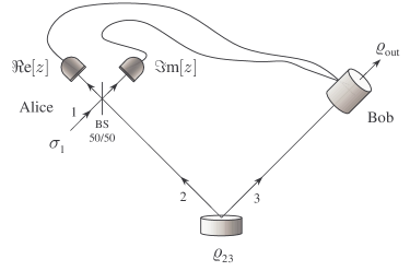
Figure 7.1: Continuous variable quantum teleportation: scheme of the optical realization.

The original proposal for teleportation concerned states in a bidimensional Hilbert space [143]. The corresponding experiments have been performed in the optical domain, using polarization qubit [144, 145], and for the state of a trapped ion [146]. Also CVQT can be realized by optical means [142], and successful teleportation of coherent states has been realized [27]. In optical CVQT, entanglement is provided by the twin-beam state (TWB) of radiation $|\Lambda\rangle\rangle_{23}=\sqrt{1-\lambda^{2}}\sum_{n=0}^{\infty}\lambda^{n}|n\rangle_{2}|n\rangle_{3}$, $2$ and $3$ being two modes of the field and $\lambda$ the TWB parameter. We assume $\lambda$ as real $|\lambda|<1$. TWBs $|\Lambda\rangle\rangle_{23}$ are produced by optical amplifiers (see Section 1.4.4) and, being a pure state, their entanglement can be quantified by the excess von Neumann entropy. We refer to Section 3.1 for details and just remind that the degree of entanglement is a monotonically increasing function of $\lambda$ (or equivalently of the average number of photons). As we will see, the larger is the entanglement the higher (closer to unit) is the fidelity of teleportation based. There are different ways to describe CVQT [142, 147, 148], but, in general, two of them are the most common: the first makes use of photon number-state basis, the other is in terms of Wigner functions. This Section addresses the description of CVQT protocol following these two approaches and, in particular, we derive the completely positive (CP) map $\mathcal{L}$ describing the teleportation process also in the presence of noise.

7.1.1 Photon number-state basis representation

Here we describe the teleportation protocol in the photon number basis. The state Alice wishes to teleport to Bob is described by the density matrix

$$\sigma_{1}=\sum_{p,q}\>\sigma_{pq}\>|p\rangle_{1}{}_{1}\langle q|\,,\;$$ (7.1)

while the pure two-mode state they share is (in general)

$$\varrho_{23}=|{\boldsymbol{C}}\rangle\rangle_{23}{}_{32}\langle\langle{\boldsymbol{C}}|\,,\quad|{\boldsymbol{C}}\rangle\rangle_{23}=\sum_{h,k}\>c_{hk}\>|h\rangle_{2}|k\rangle_{3}\;,$$ (7.2)

where we used the matrix notation introduced in Section 1.2.

The first step of the protocol consists in Alice’s joint measurement on modes 1 and 2, which corresponds to the measure of the complex photocurrent $Z=a_{1}+a_{2}^{{\dagger}}$ (see Section 5.6.1). The whole measurement process is described by the POVM

$$\Pi_{12}(z)=\frac{1}{\pi}\>D_{1}(z)|\mathbbm{1}\rangle\rangle_{12}{}_{21}\langle\langle\mathbbm{1}|D_{1}^{{\dagger}}(z)\,,\;$$ (7.3)

where $|\mathbbm{1}\rangle\rangle_{12}\equiv\sum_{v}\>|v\rangle_{1}|v\rangle_{2}$, and $D_{1}(z)$ is a displacement operator on mode 1 (see Section 5.6.4). The conditional state of mode 3 is then

$$\varrho_{3}(z) =\frac{1}{p(z)}\>{\rm Tr}_{12}\left[\sigma_{1}\otimes\varrho_{23}\>\Pi_{12}(z)\otimes\mathbb{I}_{3}\right]$$ (7.4)

$$=\frac{1}{\pi p(z)}\>{\rm Tr}_{12}\Bigg{[}\Bigg{(}\sum_{p,q}\>\sigma_{pq}|p\rangle_{1}{}_{1}\langle q|\Bigg{)}\otimes\Bigg{(}\sum_{h,k}\>\sum_{n,m}\>c_{hk}\>c^{*}_{nm}|h\rangle_{2}|k\rangle_{3}{}_{3}\langle m|{}_{2}\langle n|\Bigg{)}$$

$$\mbox{}\hskip 56.9055pt\times D_{1}(z)\Bigg{(}\sum_{v,w}\>|v\rangle_{1}|v\rangle_{2}{}_{2}\langle w|{}_{1}\langle w|\Bigg{)}D_{1}^{{\dagger}}(z)\Bigg{]}$$ (7.5)

$$=\frac{1}{\pi p(z)}\>{\rm Tr}_{12}\Bigg{[}\sum_{p,q}\>\sum_{h,k}\>\sum_{n,m}\>\sum_{v,w}\>\sigma_{pq}\>c_{hk}\>c^{*}_{nm}\>\underbrace{{}_{2}\langle n|v\rangle_{2}}_{\delta_{n,v}}\>{}_{1}\langle q|D_{1}(z)|v\rangle_{1}$$

$$\mbox{}\hskip 56.9055pt\times|k\rangle_{3}{}_{3}\langle m|\otimes|h\rangle_{2}{}_{2}\langle w|\otimes|p\rangle_{1}{}_{1}\langle w|D_{1}^{{\dagger}}(z)\Bigg{]}$$ (7.6)

$$=\frac{1}{\pi p(z)}\>\sum_{p,q}\>\sum_{h,k}\>\sum_{n,m}\>\sigma_{pq}\>c_{hk}\>c^{*}_{nm}\>{}_{1}\langle q|D_{1}(z)|n\rangle_{1}\>{}_{1}\langle h|D_{1}^{{\dagger}}(z)|p\rangle_{1}\,|k\rangle_{3}{}_{3}\langle m|$$

$$=\frac{1}{\pi p(z)}\>{\boldsymbol{C}}^{\scriptscriptstyle T}D^{{\dagger}}(z)\>\sigma\>D(z)\>{\boldsymbol{C}}^{*}\,,$$ (7.7)

where $(\cdots)^{\scriptscriptstyle T}$ denotes transposition, the subscripts have been suppressed, and $p(z)$ is the double-homodyne probability density, given by

$$p(z)={\rm Tr}_{123}\left[\sigma_{1}\otimes\varrho_{23}\>\Pi_{12}(z)\otimes\mathbb{I}_{3}\right]\,.$$ (7.8)

After the measurement, Alice sends her result to Bob through a classical channel and, then, he applies a displacement $D(z)$ to his mode, in formula:

$$\varrho_{3}(z)\rightarrow\varrho^{\prime}_{3}(z)\equiv D(z)\>\varrho_{3}(z)\>D^{{\dagger}}(z)\,.$$ (7.9)

If the entangled channel is provided by the TWB, then ${\boldsymbol{C}}=(1-\lambda^{2})^{1/2}\>\lambda^{a^{{\dagger}}a}$ and Eq. (7.9) rewrites as

$$\varrho^{\prime}_{3}(z)=\frac{(1-\lambda^{2})}{\pi p(z)}\>D(z)\>\lambda^{a^{{\dagger}}a}\>D^{{\dagger}}(z)\>\sigma\>D(z)\>\lambda^{a^{{\dagger}}a}\>D^{{\dagger}}(z)\,.$$ (7.10)

Now, using the operatorial identity (1.57), Eq. (7.10) can be reduced to

$$\varrho^{\prime}_{3}(z)=\frac{(1-\lambda^{2})}{\pi p(z)}\>\int_{\mathbb{C}^{2}}\frac{d^{2}w\>d^{2}v}{\pi^{2}(1-\lambda)^{2}}\>\exp\left\{-\frac{1}{2}\frac{1+\lambda}{1-\lambda}\>\big{(}|w|^{2}+|v|^{2}\big{)}\right\}\\ \times D(z)\>D(w)\>D^{{\dagger}}(z)\>\sigma\>D(z)\>D^{{\dagger}}(v)\>D^{{\dagger}}(z)\,,\;$$ (7.11)

which, thanks to (1.51), becomes

$$\varrho^{\prime}_{3}(z)=\frac{(1+\lambda)}{\pi p(z)}\>\int_{\mathbb{C}^{2}}\frac{d^{2}w\>d^{2}v}{\pi^{2}(1-\lambda)}\>\exp\left\{-\frac{1}{2}\frac{1+\lambda}{1-\lambda}\big{(}|w|^{2}+|v|^{2}\big{)}\right\}\\ \times\>\exp\left\{(w-v)^{*}z-(w-v)z^{*}\right\}\>D(w)\>\sigma\>D^{{\dagger}}(v)\,.$$ (7.12)

The final output of CVQT is obtained integrating $\varrho^{\prime}_{3}$ over all the possible outcomes $z$ of the double-homodyne detection, i.e.

$$\varrho_{\rm out}=\int_{\mathbb{C}}d^{2}z\>p(z)\>\varrho^{\prime}_{3}(z)\,,$$ (7.13)

and, remembering the definition (1.52) of the delta function $\delta^{(2)}(\xi)$, we obtain

$$\varrho_{\rm out}=\int_{\mathbb{C}}\frac{d^{2}w}{4\pi\sigma_{-}^{2}}\>\exp\left\{-\frac{|w|^{2}}{4\sigma_{-}^{2}}\right\}\>D(w)\>\sigma\>D^{{\dagger}}(w)\,,\;$$ (7.14)

with

$$\sigma_{-}^{2}\equiv\frac{1}{4}\frac{1-\lambda}{1+\lambda}=\frac{1}{4}\,e^{-2r}\,,$$

$r=\tanh^{-1}\lambda$ being the squeezing parameter of the TWB. Eq. (7.14) corresponds to an overall Gaussian noise with parameter $\sigma_{-}^{2}$ (see Section 4.2): in this way the CVQT protocol can be seen as a thermalizing quantum channel [149]. Notice that $\varrho_{\rm out}$ approaches the input state $\sigma$ only for $\lambda\to 1$ (or $r\to\infty$), i.e. for a TWB with infinite energy.

7.1.2 The completely positive map of CVQT

CVQT corresponds to a Gaussian completely positive (CP) map and, as we will see in Section 7.1.6, this result holds also in the presence of noise. If $\varrho_{\rm in}$ is the state at Alice’s side, the state at Bob’s side will be

$$\varrho_{\rm out}=\mathcal{L}\varrho_{\rm in}\equiv\int_{\mathbb{C}}d^{2}w\>\frac{\exp\left\{-\boldsymbol{w}^{\scriptscriptstyle T}\,\boldsymbol{\Sigma}^{-1}\,\boldsymbol{w}\right\}}{\pi\sqrt{{\rm Det}[\boldsymbol{\Sigma}]}}\>D(w)\>\varrho_{\rm in}\>D^{{\dagger}}(w)\;,$$ (7.15)

$\boldsymbol{w}$ denoting the vector $(\Re\mbox{e}[w],\Im\mbox{m}[w])^{\scriptscriptstyle T}$, and $\boldsymbol{\Sigma}$ is a $2\times 2$ matrix describing a Gaussian noise, as we have addressed in Section 4.2. Notice that Eq. (7.15) provides already the Kraus diagonal form of the teleportation map. In Section 7.1.6 we will explicitly derive the map (7.15) for teleportation in the presence of noise. In the case of Eq. (7.14) one has

$$\boldsymbol{\Sigma}=\boldsymbol{\Sigma}_{0}\equiv 4\left(\begin{array}[]{cc}\sigma_{-}^{2}&0\\ 0&\sigma_{-}^{2}\end{array}\right)\,.$$ (7.16)

7.1.3 CVQT as conditional measurement on the TWB

As we have seen in Section 5.6.4, when the modes in the measurement of $Z$ are initially excited in a factorized state, then we can write the POVM as a single-mode POVM depending on the state of the other mode. This is the case of CVQT, which can be seen as the measurement of the POVM [see Eq. (5.124)]

$$\Pi_{2}(z)=\frac{1}{\pi}\,D_{2}^{\scriptscriptstyle T}(z)\>\sigma^{\scriptscriptstyle T}\>D^{*}_{2}(z)\,,$$ (7.17)

acting on the mode 2: in this way CVQT is reduced to a conditional measurement on the TWB followed by a displacement. Let $\sigma$ be again the state we wish to teleport and let the TWB be the entangled state shared between Alice and Bob. The conditioned state of mode 2 is then (we put $\varrho_{\hbox{\tiny TWB}}\equiv\varrho_{23}$)

$$\varrho_{3}(z) =\frac{1}{p(z)}\>{\rm Tr}_{2}\left[\varrho_{\hbox{\tiny TWB}}\>\Pi_{2}(z)\otimes\mathbb{I}\right]$$

$$=\frac{(1-\lambda^{2})}{\pi p(z)}\>{\rm Tr}_{2}\left[\sum_{h,k}\>\lambda^{h+k}\>|h\rangle_{2}|h\rangle_{3}{}_{3}\langle k|{}_{2}\langle k|D_{2}^{\scriptscriptstyle T}(z)\>\sigma^{\scriptscriptstyle T}\>D^{*}_{2}(z)\right]$$

$$=\frac{(1-\lambda^{2})}{\pi p(z)}\>\sum_{h,k}\>\lambda^{h+k}\>{}_{2}\langle k|D_{2}^{\scriptscriptstyle T}(z)\>\sigma^{\scriptscriptstyle T}\>D^{*}_{2}(z)|h\rangle_{2}\>|h\rangle_{3}{}_{3}\langle k|\,,$$ (7.18)

with the double-homodyne density probability distribution $p(z)$ given by

$$p(z)={\rm Tr}_{23}\left[\varrho_{\hbox{\tiny TWB}}\>\Pi_{2}(z)\otimes\mathbb{I}\right]\,.$$ (7.19)

Since $[D^{\scriptscriptstyle T}(z)]^{*}=D^{{\dagger}}(z)$, in Eq. (7.18) we can write

$${}_{2}\langle k|D_{2}^{\scriptscriptstyle T}(z)\>\sigma^{\scriptscriptstyle T}\>D^{*}_{2}(z)|h\rangle_{2} ={}_{2}\langle k|\big{[}D_{2}^{{\dagger}}(z)\>\sigma\>D_{2}(z)\big{]}^{\scriptscriptstyle T}|h\rangle_{2}$$

$$={}_{2}\langle h|D_{2}^{{\dagger}}(z)\>\sigma\>D_{2}(z)|k\rangle_{2}\,,\;$$ (7.20)

and, suppressing all the subscripts, we have

$$\varrho_{3}(z)=\frac{(1-\lambda^{2})}{\pi p(z)}\>\sum_{h,k}\>\lambda^{h+k}\>\langle h|D^{{\dagger}}(z)\>\sigma\>D(z)|k\rangle\>|h\rangle\langle k|\,.$$ (7.21)

In order to have a full quantum teleportation, we must displace the state (7.21) applying $D(z)$, obtaining

$$\varrho^{\prime}_{3}(z) =D(z)\>\varrho_{3}(z)\>D^{{\dagger}}(z)$$

$$=\frac{(1-\lambda^{2})}{\pi p(z)}\>\sum_{h,k}\>\lambda^{h+k}\>\langle h|D^{{\dagger}}(z)\>\sigma\>D(z)|k\rangle\>D(z)|h\rangle\langle k|D^{{\dagger}}(z)$$ (7.22)

$$=\frac{(1-\lambda^{2})}{\pi p(z)}\>\sum_{h,k}\>\lambda^{h+k}\>\langle\psi_{h}(z)|\sigma|\psi_{k}(z)\rangle\>|\psi_{h}(z)\rangle\langle\psi_{k}(z)|\,,$$ (7.23)

where we defined the new s.o.n.c. $\left\{|\psi_{h}(z)\rangle\right\}$, with $|\psi_{h}(z)\rangle\equiv D(z)|h\rangle$. Notice that Eq. (7.22) can be written in operational form as

$$\varrho^{\prime}_{3}(z) =\frac{(1-\lambda^{2})}{\pi p(z)}\>\sum_{h,k}\>\lambda^{h+k}\>D(z)|h\rangle\langle h|D^{{\dagger}}(z)\>\sigma\>D(z)|k\rangle\>\langle k|D^{{\dagger}}(z)$$

$$=\frac{(1-\lambda^{2})}{\pi p(z)}\>\sum_{h,k}\>\>D(z)|h\rangle\lambda^{a^{{\dagger}}a}\langle h|D^{{\dagger}}(z)\>\sigma\>D(z)|k\rangle\>\langle k|\lambda^{a^{{\dagger}}a}D^{{\dagger}}(z)$$

$$=\frac{(1-\lambda^{2})}{\pi p(z)}\>D(z)\>\lambda^{a^{{\dagger}}a}\>D^{{\dagger}}(z)\>\sigma\>D(z)\>\lambda^{a^{{\dagger}}a}\>D^{{\dagger}}(z)\,,$$ (7.24)

which is the same as in Eq. (7.10). Finally, $\varrho_{\rm out}$ is obtained by means of Eq. (7.13).

7.1.4 Wigner functions representation

This Section addresses CVQT described in terms of Wigner functions. We first derive the teleported state Wigner function when the shared state has the general form given in Eq. (7.2), then we specialize the results to the case of a TWB.

Let $W[\sigma](\alpha_{1})$ and $W[\varrho_{23}](\alpha_{2},\alpha_{3})$ be the Wigner functions associated to the states (7.1) and (7.2), respectively, where $\alpha_{h}=\kappa_{2}(x_{h}+iy_{h})$ (see Chapter 1). Since the Wigner function corresponding to the POVM of ideal double- homodyne detection on mode 1 and 2 is

$$W[\Pi_{12}(z)](\alpha_{1},\alpha_{2})=\frac{1}{\pi^{2}}\>\delta^{(2)}\big{(}(\alpha_{1}-\alpha_{2}^{*})-z\big{)}\,,\;$$ (7.25)

with $z=\kappa_{2}(x+iy)$, using Eq. (1.133) the double-homodyne density probability distribution (7.8) reads

$$p(z)=\pi^{3}\,\int_{\mathbb{C}^{3}}d^{2}\alpha_{1}\,d^{2}\alpha_{2}\,d^{2}\alpha_{3}\,W[\sigma](\alpha_{1})\,W[\varrho_{23}](\alpha_{2},\alpha_{3})\,W[\Pi_{12}(z)](\alpha_{1},\alpha_{2})\>W[\mathbb{I}_{3}](\alpha_{3})\,,\;$$ (7.26)

while the conditioned state of mode 3 is

$$W[\varrho_{3}(z)](\alpha_{3})=\frac{\pi^{2}}{p(z)}\>\int_{\mathbb{C}^{2}}d^{2}\alpha_{1}\,d^{2}\alpha_{2}\>W[\sigma](\alpha_{1})\>W[\varrho_{23}](\alpha_{2},\alpha_{3})\,W[\Pi_{12}(z)](\alpha_{1},\alpha_{2})\,W[\mathbb{I}_{3}](\alpha_{3})\,,$$ (7.27)

where $W[\mathbb{I}_{3}](\alpha_{3})=\pi^{-1}$. Thanks to Eq. (7.25) and after the integration over $\alpha_{1}$, Eq. (7.27) becomes

$$W[\varrho_{3}(z)](\alpha_{3}) =\frac{1}{\pi p(z)}\>\int_{\mathbb{C}}d^{2}\alpha_{2}\,\>W[\sigma](\alpha_{2}^{*}+z)\>W[\varrho_{23}](\alpha_{2},\alpha_{3})$$

$$=\frac{1}{\pi p(z)}\>\int_{\mathbb{C}}d^{2}\alpha_{2}\>W[\sigma](\alpha_{2})\>W[\varrho_{23}](\alpha_{2}^{*}-z^{*},\alpha_{3})\,.$$ (7.28)

Now we perform the displacement $D(z)$, on mode 3, obtaining

$$W[\varrho^{\prime}_{3}(z)](\alpha_{3})=\frac{1}{\pi p(z)}\>\int_{\mathbb{C}}d^{2}\alpha_{2}\>W[\sigma](\alpha_{2})\>W[\varrho_{23}](\alpha_{2}^{*}-z^{*},\alpha_{3}-z)\,.$$ (7.29)

with $\varrho^{\prime}_{3}(z)\equiv D(z)\>\varrho_{3}(z)\>D^{{\dagger}}(z)$, and where we used the property (1.143b). The output state of CVQT is obtained integrating Eq. (7.29) over all the possible outcomes of the double homodyne detection, namely

$$W[\varrho_{\rm out}](\alpha_{3})=\int_{\mathbb{C}}d^{2}z\>p(z)\>W[\varrho^{\prime}_{3}(z)](\alpha_{3})\,.$$ (7.30)

If the shared state is the TWB, the Wigner function reads as follows

$$W[{\varrho_{23}}](\alpha_{2},\alpha_{3})=\frac{\exp\left\{-\frac{1}{2}\,\boldsymbol{\alpha}_{23}^{\scriptscriptstyle T}\,\boldsymbol{\sigma}_{\boldsymbol{\alpha}}^{-1}\,\boldsymbol{\alpha}_{23}\right\}}{(2\,\pi)^{2}\sqrt{{\rm Det}[\boldsymbol{\sigma}_{\boldsymbol{\alpha}}]}}$$ (7.31)

with $\boldsymbol{\alpha}_{hk}\equiv\big{(}\Re\mbox{e}[\alpha_{h}],\Im\mbox{m}[\alpha_{h}],\Re\mbox{e}[\alpha_{k}],\Im\mbox{m}[\alpha_{k}]\big{)}^{\scriptscriptstyle T}$ and

$$\boldsymbol{\sigma}_{\boldsymbol{\alpha}}=\frac{1}{2}\left(\begin{array}[]{cc}(\sigma_{+}^{2}+\sigma_{-}^{2})\,{\mathbbm{1}}_{2}&(\sigma_{+}^{2}-\sigma_{-}^{2})\,\boldsymbol{\sigma}_{3}\\[4.30554pt] (\sigma_{+}^{2}-\sigma_{-}^{2})\,\boldsymbol{\sigma}_{3}&(\sigma_{+}^{2}+\sigma_{-}^{2})\,{\mathbbm{1}}_{2}\end{array}\right)\,,$$ (7.32)

${\mathbbm{1}}_{2}$ being the $2\times 2$ identity matrix, $\sigma_{\pm}^{2}=\frac{1}{4}e^{\pm 2r}$, $\boldsymbol{\sigma}_{3}={\rm Diag}(1,-1)$ is a Pauli matrix, and $r=\tanh^{-1}\lambda$ is the squeezing parameter of the TWB. Substituting Eq. (7.31) into Eq. (7.29) and integrating over $z$ one has

$$W[\varrho_{\rm out}](\alpha_{3}) =\int_{\mathbb{C}}\frac{d^{2}\alpha_{2}}{4\pi\sigma_{-}^{2}}\>\exp\left\{-\frac{|\alpha_{2}-\alpha_{3}|^{2}}{4\sigma_{-}^{2}}\right\}\>W[\sigma](\alpha_{2})$$ (7.33)

$$=\int_{\mathbb{C}}d^{2}w\>\frac{\exp\left\{-\boldsymbol{w}^{\scriptscriptstyle T}\,\boldsymbol{\Sigma}^{-1}\,\boldsymbol{w}\right\}}{\pi\sqrt{{\rm Det}[\boldsymbol{\Sigma}]}}\>W[D(w)\>\sigma\>D^{{\dagger}}(w)](\alpha_{3})\,,$$ (7.34)

with $w\equiv\alpha_{2}$, $\boldsymbol{w}=(\Re\mbox{e}[w],\Im\mbox{m}[w])^{\scriptscriptstyle T}$, and $\boldsymbol{\Sigma}\equiv\boldsymbol{\Sigma}_{0}$ is given in Eq. (7.16). Finally, using Eq. (1.134), we obtain the same density matrix as in Eq. (7.15).

7.1.5 Teleportation fidelity

Teleportation has occurred when the output signal $\varrho_{\rm out}$ is in the same quantum state of the unknown input $\sigma$. Therefore, we need to define a quantity which gauges the similarity between $\sigma$ and $\varrho_{\rm out}$. This task is achieved using the so called “fidelity” or “average fidelity” between the input and output state. When the input signal is a pure state $\sigma=|\psi\rangle\langle\psi|$ the fidelity is defined in the following way [152]

$$\overline{F} \equiv{\rm Tr}[\sigma\>\varrho_{\rm out}]=\langle\psi|\varrho_{\rm out}|\psi\rangle\>,$$ (7.35a)

$$\overline{F} \equiv\pi\int_{\mathbb{C}}d^{2}\alpha\>W[\sigma](\alpha)\>W[\varrho_{\rm out}](\alpha)\,,\;$$ (7.35b)

in terms of density matrix and Wigner function representation, respectively. $\overline{F}$ has the property that it equals 1 if and only if $\sigma$ is a pure state and $\varrho_{\rm out}=\sigma$; on the other hand, it equals 0 if and only if the input and output states can be distinguished with certainty by some quantum measurement. In particular the average fidelity evaluates the extent at which all possible measurement statistics produceable by the output state match the corresponding statistics produceable by the input state. In order to explain this last consideration, let us consider the generic POVM $\{\Pi_{\alpha}\}$, describing a certain observable, with measurement outcomes $\alpha$. If the observable were performed on the input system, it would give a probability density for the outcomes $\alpha$ given by

$$P_{\rm in}(\alpha)={\rm Tr}[\sigma\>\Pi_{\alpha}]\,;\;$$ (7.36)

if the same observable were performed on the output system, it would give, instead, the probability density

$$P_{\rm out}(\alpha)={\rm Tr}[\varrho_{\rm out}\>\Pi_{\alpha}]\,.\;$$ (7.37)

Now, a natural way to gauge the similarity of these two probability densities is by their overlap $\mathcal{Q}$, defined as follows

$$\mathcal{Q}=\int_{\mathbb{C}}d^{2}\alpha\>\sqrt{P_{\rm in}(\alpha)\>P_{\rm out}(\alpha)}\;.$$ (7.38)

It turns out that regardless of which observable is being considered $\mathcal{Q}\geq\overline{F}$ and, moreover, one can show [150] that there exists an observable that gives precise equality in this expression.

When the shared state is the TWB, substituting Eq. (7.14) into the Eq. (7.35a), one straightforward obtains

$$\overline{F}_{\hbox{\tiny TWB}}(\lambda)\equiv\overline{F}(\lambda)=\frac{1}{1+4\>\sigma_{-}^{2}}=\frac{1+\lambda}{2}\;.$$ (7.39)

The maximum average fidelity achievable by means of some classical (local) procedure to teleport a state is known as classical limit. This procedure should be characterized by a local measurement on the state to be teleported, a classical communication of the result, say $\mathcal{R}$, and, finally, a preparation stage at the receiver, according to a rule that associates a certain output state to $\mathcal{R}$ such that fidelity is maximized.

Let us suppose that Alice wishes to transmit to Bob an unknown coherent state without the resource of entanglement, i.e. by no means of a shared entangled state. In such a case, we are interested in evaluating the maximum average fidelity achievable. First of all we assume that the coherent state is drawn from the set $\cal S$ constituted by the coherent states $|\beta\rangle$,where the complex parameter $\beta$ is distributed according to the Gaussian distribution

$$p(\beta)=\frac{\Omega}{\pi}\,e^{-\Omega|\beta|^{2}}\;,$$ (7.40)

$\Omega$ being a real, positive parameter. Ultimately, of course, we would like to consider the case where Alice and Bob have no information about the drown coherent state: this is simply described by taking the limit $\Omega\rightarrow 0$.

Alice’s measurement for estimating the unknown parameter $\beta$ when it is distributed according to a Gaussian distribution [151] is the POVM $\{\Pi_{z}\}$ constructed from the coherent state projectors according to $\Pi_{z}=\pi^{-1}|z\rangle\langle z|$: this kind of measurement is equivalent to optical heterodyning described in Section 5.6.4, where we send the vacuum in the other detector input port [see Eq. (5.122) with $\tau=|0\rangle\langle 0|$]. As in the case of the teleportation protocol, Alice’s measurement outcome $z$ is classically sent to Bob, that generates a new quantum state according to the rule $z\rightarrow|f_{z}\rangle$. Let us make no a priori restrictions on the states $|f_{z}\rangle$.

Now, we find the maximum average fidelity $\overline{F}_{\rm max}(\Omega)$ Bob can achieve for a given $\Omega$. For a given strategy $z\rightarrow|f_{z}\rangle$, the achievable average fidelity is [152]

$$\overline{F}(\Omega) =\int_{\mathbb{C}}d^{2}\beta\,p(\beta)\int_{\mathbb{C}}d^{2}z\,p(z|\beta)\,|\langle f_{z}|\beta\rangle|^{2}=\frac{\Omega}{\pi^{2}}\int_{\mathbb{C}^{2}}d^{2}z\,d^{2}\beta\,e^{-\Omega|\beta|^{2}}\,e^{-|z-\beta|^{2}}|\langle f_{z}|\beta\rangle|^{2}$$

$$=\frac{\Omega}{\pi^{2}}\int_{\mathbb{C}}d^{2}z\,e^{-|z|^{2}}\langle f_{z}|{\cal O}_{z}(\Omega)|f_{z}\rangle\;,$$ (7.41)

where $p(z|\beta)={\rm Tr}[|\beta\rangle\langle\beta|\,\Pi_{z}]$ is the heterodyne probability density distribution and we defined the positive semi-definite Hermitian operator

$${\cal O}_{z}(\Omega)\equiv\int_{\mathbb{C}}d^{2}\beta\,\exp\Big{\{}-(1+\Omega)|\beta|^{2}+2\Re{\rm e}[z^{*}\beta]\Big{\}}\,|\beta\rangle\langle\beta|\;,$$ (7.42)

that depends only on the real parameter $\Omega$ and the complex parameter $z$. It follows that

$$\langle f_{z}|{\cal O}_{z}(\Omega)|f_{z}\rangle\leq\max\big{[}{\cal O}_{z}(\Omega)\big{]}\;,$$ (7.43)

where $\max[X]$ denotes the largest eigenvalue of the operator $X$.

Now, for each $z$, Bob adjusts the state $|f_{z}\rangle$ to be the eigenvector of ${\cal O}_{z}(\Omega)$ with the largest eigenvalue. Then equality is achieved in Eq. (7.43) and it is just a question of being able to perform the integral in Eq. (7.41). The first step in carrying this out is to find the eigenvector and the eigenvalue achieving equality in Eq. (7.43). This is most easily evaluated by unitarily transforming ${\cal O}_{z}(\Omega)$ into a new operator diagonal in the number basis, picking off the largest eigenvalue and transforming back to get the optimal $|f_{z}\rangle$ (we remember that eigenvalues are invariant under unitary transformations).

In order to find the largest eigenvalue of ${\cal O}_{z}(\Omega)$, we consider the positive operator

$$P=\int_{\mathbb{C}}d^{2}\beta\,e^{-(1+\Omega)|\beta|^{2}}|\beta\rangle\langle\beta|\,.$$ (7.44)

Since the number basis expansion of $P$ has the following diagonal form

$$P =\int_{\mathbb{C}}d^{2}\beta\,e^{-(1+\Omega)|\beta|^{2}}\,\sum_{n,m}\frac{e^{-|\beta|^{2}}}{\sqrt{n!\,m!}}\,\beta^{n}\,(\beta^{*})^{m}\,|n\rangle\langle m|$$

$$=\sum_{n,m}\frac{1}{\sqrt{n!\,m!}}\underbrace{\int_{0}^{2\pi}d\phi\,e^{i\phi(n-m)}}_{\displaystyle 2\pi\delta_{n,m}}\int_{0}^{\infty}d\rho\,\rho^{n+m+1}\,e^{-(2+\Omega)\rho^{2}}\,|n\rangle\langle m|$$

$$=\sum_{n}\frac{2\pi}{n!}\underbrace{\int_{0}^{\infty}d\rho\,\rho^{2n+1}\,e^{-(2+\Omega)\rho^{2}}}_{\displaystyle\mbox{$\frac{1}{2}$}n!\,(2+\Omega)^{-(n+1)}}\,|n\rangle\langle n|=\pi\sum_{n=0}^{\infty}(2+\Omega)^{-(n+1)}|n\rangle\langle n|\;,$$ (7.45)

its eigenvalues are $\{\pi\,(2+\Omega)^{-(n+1)}\}$ and, then, $\mu(P)=\pi/(2+\Omega)$, i.e. the vacuum state’s eigenvalue.

Now consider the displaced operator

$$Q_{z}(\Omega)=D\!\left(\frac{z}{1+\Omega}\right)P\,D^{\dagger}\!\left(\frac{z}{1+\Omega}\right)\;,$$ (7.46)

where $D(\nu)$ is the standard displacement operator. Using Eq. (7.44), one finds

$$Q_{z}(\Omega) =\int_{\mathbb{C}}d^{2}\beta\,\exp\left\{-(1+\Omega)|\beta|^{2}\right\}\left|\beta+\frac{z}{1+\Omega}\right\rangle\left\langle\beta+\frac{z}{1+\Omega}\right|$$

$$=\int_{\mathbb{C}}d^{2}\xi\,\exp\left\{-(1+\Omega)\left|\xi-\frac{z}{1+\Omega}\right|^{2}\,\right\}|\xi\rangle\langle\xi|$$

$$=\exp\left\{-\frac{|z|^{2}}{1+\Omega}\right\}\int_{\mathbb{C}}d^{2}\xi\,\exp\Big{\{}-(1+\Omega)|\xi|^{2}+2\Re{\rm e}[z^{*}\xi]\Big{\}}|\xi\rangle\langle\xi|\,$$

$$=\exp\left\{-\frac{|z|^{2}}{1+\Omega}\right\}\,{\cal O}_{z}(\Omega)\;,$$ (7.47)

and, substituting this into Eq. (7.41), we have

$$\overline{F}(\Omega) =\frac{\Omega}{\pi^{2}}\int_{\mathbb{C}}d^{2}z\,\exp\left\{-\left(1-\frac{1}{1+\Omega}\right)|z|^{2}\right\}\langle f_{z}|Q_{z}(\Omega)|f_{z}\rangle$$

$$\leq\frac{1}{\pi}\frac{\Omega}{2+\Omega}\int_{\mathbb{C}}d^{2}z\,\exp\left\{-\frac{\Omega}{1+\Omega}|z|^{2}\right\}=\frac{1+\Omega}{2+\Omega}\;.$$ (7.48)

Equality is obviously achieved in the previous expression by taking

$$|f_{z}\rangle=D\!\left(\frac{z}{1+\Omega}\right)|0\rangle=\left|\frac{z}{1+\Omega}\right\rangle\,;$$ (7.49)

therefore the maximum average fidelity is given by

$$\overline{F}_{\rm max}(\Omega)=\frac{1+\Omega}{2+\Omega}\;.$$ (7.50)

For $\Omega\rightarrow\infty$ we have $\overline{F}_{\rm max}(\Omega)\rightarrow 1$ since this situation corresponds to the teleportation of a single known coherent state, a task that can be achieved classically by transmitting the value of the amplitude. On the other hand, in the limit $\Omega\rightarrow 0$, i.e. when the coherent state to be sent is drawn from a uniform distribution, we have $\overline{F}_{\rm max}(\Omega)\to 1/2$.

It should be noted that nothing in this argument depended upon the mean of the Gaussian distribution being $\beta=0$: Bob would need to minimally modify his strategy to take into account Gaussians with a non-vacuum state mean, but the optimal fidelity would remain the same.

7.1.6 Effect of noise

In this Section we study CVQT assisted by a TWB propagating through a squeezed-thermal environment. Taking into account the results obtained in Section 4.4, the teleported state is now obtained from Eq. (7.34) with

$$\boldsymbol{\Sigma}\equiv\boldsymbol{\Sigma}(\Gamma,N_{\rm th},N_{\rm s})=4\left(\begin{array}[]{cc}\Sigma_{3}^{2}&0\\ 0&\Sigma_{2}^{2}\end{array}\right)\,,$$ (7.51)

$\Sigma_{2}^{2}$, $\Sigma_{3}^{2}$ being given in Eqs. (4.49).

Finally, non-unit quantum efficiency $\eta$ in the joint measurement modifies the POVM, which becomes a Gaussian convolution of the ideal one, as pointed out in Chapter 5. In this case the output state is given by Eq. (7.34) where

$$\boldsymbol{\Sigma}\equiv\boldsymbol{\Sigma}(\Gamma,N_{\rm th},N_{\rm s},\eta)=\left(\begin{array}[]{cc}4\,\Sigma_{3}^{2}+D_{\eta}^{2}&0\\ 0&4\,\Sigma_{2}^{2}+D_{\eta}^{2}\end{array}\right)\,,$$ (7.52)

with $D_{\eta}^{2}=(1-\eta)/\eta$ [96].

7.1.7 Optimized teleportation in the presence of noise

In order to use CVQT as a resource for quantum information processing, we look for a class of squeezed states which achieves an average teleportation fidelity greater than the one obtained teleporting coherent states in the same conditions. If the input squeezed state to be teleported is $\sigma=|\alpha,\xi\rangle\langle\alpha,\xi|$, $|\alpha,\xi\rangle=D(\alpha)S(\xi)|0\rangle$, then the teleported state given by Eq. (7.34) has average teleportation fidelity [see Eq. (7.35b)]

$$\overline{F}_{\xi}(\lambda)=\Big{(}\sqrt{(e^{2\xi}+4\>\Sigma_{2}^{2})(e^{-2\xi}+4\>\Sigma_{3}^{2})}\Big{)}^{-1}\,,$$ (7.53)

which attains its maximum

$$\overline{F}(\lambda)=(1+4\>\Sigma_{2}\>\Sigma_{3})^{-1}\,,$$ (7.54)

when

$$\xi=\xi_{\rm max}\equiv\frac{1}{2}\ln\left(\frac{\Sigma_{2}}{\Sigma_{3}}\right)\,.$$ (7.55)

For non squeezed environment $N_{\rm s}\rightarrow 0$ we have $\Sigma_{2}=\Sigma_{3}$, and thus then $\xi_{\rm max}\rightarrow 0$, i.e. the input state that maximizes the average fidelity (7.53) reduces to a coherent state. In other words, in a non squeezed environment the teleportation of coherent states is more effective than that of squeezed states. Moreover, Eq. (7.54) shows that meanwhile the TWB becomes separable, i.e. $\Sigma_{2}^{2}\>\Sigma_{3}^{2}\geq 16^{-1}$ [see Eqs. (4.51)], one has $\overline{F}\leq 0.5$. Finally, the asymptotic value of $\overline{F}$ for $\Gamma t\rightarrow\infty$ is

$$\overline{F}^{(\infty)}=[2\>(1+N_{\rm th})]^{-1}\,,$$ (7.56)

which does not depend on the number of squeezed photons and is equal to $0.5$ only if $N_{\rm th}=0$. This last result is equivalent to say that in the presence of a zero-temperature environment, no matter if it is squeezed or not, the TWB is non-separable at every time.

Figure 7.2: Plots of the average teleportation fidelity. The solid and the dashed lines represent squeezed and coherent state fidelity, respectively, for different values of the number of squeezed photons $N_{\rm s}$: (a) $N_{\rm s}=0$, (b) $0.1$, (c) $0.3$, (d) $0.7$. In all the plots we put the TWB parameter $\lambda=1.5$ and number of thermal photons $N_{\rm th}=0.5$. The dot-dashed vertical line indicates the threshold $\Gamma t_{\rm s}$ for the separability of the shared state: when $\Gamma t>\Gamma t_{\rm s}$ the state is no more entangled. Notice that, in the case of squeezed state teleportation, the threshold for the separability corresponds to $\overline{F}=0.5$.

In Fig. 7.2 we plot $\overline{F}_{\rm tele}$ as a function of $\Gamma t$ for different values of $\lambda$, $N_{\rm th}$ and $N_{\rm s}$. As $N_{\rm s}$ increases, the nonclassicality of the thermal bath starts to affect the teleportation fidelity and we observe that the best results are obtained when the state to be teleported is the squeezed state that maximizes (7.53). Furthermore the difference between the two fidelities increases as $N_{\rm s}$ increases. Notice that there is an interval of values for $\Gamma t$ such that the coherent state teleportation fidelity is less than the classical limit $0.5$, although the shared state is still entangled.

7.1.8 Teleportation improvement

TWBs are produced either by degenerate (with additional beam splitters) or nondegenerate optical parametric amplifiers. The TWB parameter $\lambda=\tanh r$ depends on the physical parameters as $r\propto\chi^{(2)}L$, $\chi^{(2)}$ being the nonlinear susceptibility of the crystal used as amplifying medium and $L$ the effective interaction length. For a given amplifier, the TWB parameter and thus the amount of entanglement are fixed. Therefore, since nonlinearities are small, and the crystal length cannot be increase at will, it is of interest to devise suitable quantum operations to increase entanglement and in turn to improve teleportation fidelity.

In Section 6.2.1 we have seen that the nonlocal correlations of TWB are enhanced for small energies by means of the IPS process described in Section 5.4.1: motivated by this result, we will use the IPS state (5.48) or, equivalently, (5.51) as shared entangled state between Alice and Bob. In this case, Eqs. (7.35) lead to the following expression for the average teleportation fidelity of coherent states[92]

$$\overline{F}(\lambda,\tau_{\rm eff})=\frac{1}{2}\frac{(1+\lambda)(1+\lambda\tau_{\rm eff})(1-\lambda^{2}\tau_{\rm eff})[2-2\lambda\tau_{\rm eff}+\lambda^{2}\tau_{\rm eff}]}{(1+\lambda^{2}\tau_{\rm eff})[1+(1-\tau_{\rm eff})\lambda]\{2-[2+(1-\tau_{\rm eff})\lambda]\lambda\tau_{\rm eff}\}}\>,$$ (7.57)

where $\tau_{\rm eff}=1-\eta(1-\tau)$ (see Section 5.4.1).

Figure 7.3: On the left: IPS average fidelity $\overline{F}(\lambda,\tau_{\rm eff})$ as a function of the TWB parameter $\lambda$ for different values of $\tau_{\rm eff}=1-\eta(1-\tau)$: (a) $\tau_{\rm eff}=1$, (b) $0.9$, (c) $0.8$, and (d) $0.5$; the dashed line is the average fidelity $\overline{F}_{\hbox{\tiny TWB}}(\lambda)$ for teleportation with TWB. On the right: Threshold value $\lambda_{\rm th}(\tau_{\rm eff})$ on the TWB parameter $x$ (solid line): when $\lambda<\lambda_{\rm th}$ we have $\overline{F}(\lambda,\tau_{\rm eff})>\overline{F}_{\hbox{\tiny TWB}}(\lambda)$ and teleportation is improved. The dot-dashed line is $\lambda=1/3$, which corresponds to $\overline{F}_{\hbox{\tiny TWB}}=2/3$: when fidelity is greater than 2/3 Bob is sure that his teleported state is the best existing copy of the initial state [155]. The dashed line represents the values $\lambda_{2/3}(\tau_{\rm eff})$ giving an average fidelity $\overline{F}(\lambda,\tau_{\rm eff})=2/3$. When $\lambda_{2/3}<\lambda<\lambda_{\rm th}$ both the teleportation is improved and the fidelity is greater than $2/3$.

In Fig. 7.3 we plot the average fidelity for different values of $\tau_{\rm eff}$: the IPS state improves the average fidelity of quantum teleportation when the energy of the incoming TWB is below a certain threshold, which depends on $\tau_{\rm eff}$ and, in turn, on $\tau$ and $\eta$. When $\tau_{\rm eff}$ approaches unit (when $\eta\rightarrow 1$ and $\tau\rightarrow 1$), Eq. (7.57) reduces to the result obtained by Milburn et al. in Ref. [94] and the IPS average fidelity (line labeled with “a” in Fig. 7.2) is always greater than the fidelity $\overline{F}_{\hbox{\tiny TWB}}(\lambda)$ obtained with the TWB state [see Eq. (7.39)]. However, a threshold value, $\lambda_{\rm th}(\tau_{\rm eff})$, for the TWB parameter $\lambda$ appears when $\tau_{\rm eff}<1$: only if $\lambda$ is below this threshold the teleportation is actually improved [$\overline{F}(\lambda,\tau_{\rm eff})>\overline{F}_{\hbox{\tiny TWB}}(\lambda)$], as shown in Fig. 7.3. Notice that, for $\tau_{\rm eff}<0.5$, $\overline{F}(\lambda,\tau_{\rm eff})$ is always below $\overline{F}_{\hbox{\tiny TWB}}(\lambda)$.

Ralph et al. demonstrated that entanglement is needed to achieve a fidelity greater than $1/2$ [153] and, using both the TWB and the IPS state (5.51), this limit is always reached (see Fig. 7.3). Nevertheless, we remember that in teleportation protocol the state to be teleported is destroyed during the measurement process performed by Alice, so that the only remaining copy is that obtained by Bob. When the initial state carries reserved information, it is important that the only existing copy will be the Bob’s one. On the other hand, using the usual teleportation scheme, Bob cannot avoid the presence of an eavesdropper, which can clone the state, obviously introducing some error [154], but he is able to to verify if his state was duplicated. This is possible by the analysis of the average teleportation fidelity: when fidelity is greater than $2/3$, Bob is sure that his state was not cloned [154, 155]. The dashed line in Fig. 7.3 (right) shows the values $\lambda_{2/3}(\tau_{\rm eff})$ which give an average fidelity (7.57) equal to $2/3$: notice that when $\lambda_{2/3}<\lambda<\lambda_{\rm th}$ both the teleportation is improved and the the fidelity is greater than $2/3$. Moreover, while the condition $\overline{F}_{\hbox{\tiny TWB}}(\lambda)>2/3$ is satisfied only if $\lambda>1/3$, for the IPS state there exists a $\tau_{\rm eff}$-dependent interval of $\lambda$ values ($\lambda_{\rm 2/3}<\lambda<1/3$) for which teleportation can be considered secure [$\overline{F}(\lambda,\tau_{\rm eff})>2/3$].

7.2 Quantum cloning

A fundamental difference between classical and quantum information is that the latter cannot be perfectly copied, even in principle. This means that there exist no physical process that can produce perfect copies of generic unknown quantum states. This so called no-cloning theorem emerges as an immediate consequence of the linearity of quantum dynamics [140, 141]. Remarkably, if cloning was permitted, the Heisenberg uncertainty principle would be violated by measuring conjugate observables on many copies of a single quantum state. Nevertheless, even if perfect cloning is not possible, one may attempt to attain imperfect copies of generic unknown quantum states. With an abuse of language, this is what is generally referred to as cloning process. With an $n$ to $m$ cloning process it is thus meant that $m$ imperfect copies are produced from $n$ identical original states ($m>n$). In this section we address the cloning issue for Gaussian states, first recalling the bounds that no-cloning theorem imposes in this case, then investigating some local and nonlocal (telecloning) cloning protocols.

7.2.1 Optimal universal cloning

The first concept to introduce is the universality of a cloning machine [156]. By universality we mean that the quality of the clones should be independent on the original states. As we have already seen in Section 7.1.5, we may use the fidelity as a measure of the similarity between two states, hence in a universal cloning machine every clone has the same fidelity with respect to the original state, independently of the original state itself. Furthermore, when the clones are equal one each other then we deal with symmetric cloning, while if we admit differences in the copies we have asymmetric cloning. Consider for the moment the first scenario. Universal cloning machines have been extensively studied for the case of discrete variables, for which it has been shown that the optimal $n$ to $m$ universal cloning machine of $d$-dimensional systems yields the fidelity [157]:

$$F=\frac{n(d-1)+m(n+1)}{m(n+d)}\,.$$ (7.58)

In the limit of infinite dimensional systems one can show that the optimal universal cloner reduces to a classical probability distributor, attaining $F=n/m$ [158], consistent with the $d\rightarrow\infty$ limit of Eq. (7.58). This means that a universal continuous variable cloner behaves like a simple classical device that distributes the $n$ original input states into $n$ output states, chosen by chance between the possible $m$ outputs and disregarding the remaining states. Nevertheless, a more interesting situation occur if we restrict the input states to the class of Gaussian states. Consider for the moment $n$ identical arbitrary coherent states. The imperfection of the $m$ copies may be regarded as an excess noise variance $\sigma_{n,m}^{2}$ in the quadratures, due to the $n$ to $m$ cloning process. Then, a procedure similar to what was done for qubits [159] allows one to estimate a lower bound $\overline{\sigma}_{n,m}^{2}$ on the noise variance [160]. In fact, make use of the property that cascading two cloning processes results in a single cloning process whose excess noise variance is simply the sum of the variances of the two cloning. Then, the variance $\overline{\sigma}_{n,l}^{2}$ of an optimal $n$ to $l$ cloning must satisfy $\overline{\sigma}_{n,l}^{2}\leq\sigma_{n,m}^{2}+\sigma_{m,l}^{2}$ ($n\leq m\leq l$). In particular, if the $m$ to $l$ cloner is itself optimal and $l\rightarrow\infty$, we have

$$\overline{\sigma}_{n,\infty}^{2}\leq\sigma_{n,m}^{2}+\overline{\sigma}_{m,\infty}^{2}\,.$$ (7.59)

As a matter of fact, a cloner that allows to build infinitely many copies corresponds to an optimal measurement of the original states, hence, with the aid of quantum estimation theory, one may identify $\overline{\sigma}_{n,\infty}^{2}=1/n$ (we put $\kappa_{1}=2^{-1/2}$). As a consequence, the lower bound we were looking for is given by

$$\overline{\sigma}_{n,m}^{2}=\frac{m-n}{m\,n}\,.$$ (7.60)

This result implies that the optimal cloning fidelity for coherent states is bounded by [160]

$$F_{n,m}=\frac{m\,n}{m\,n+m-n}\,.$$ (7.61)

Notice that this result does not depend on the amplitude of the input coherent states. If general squeezed states are considered, optimality can then be achieved only if the excess noise variance is squeezed by the same amount as the initial state, thus making the cloner state-dependent.

Remarkably, optimal cloners achieving the fidelity given in Eq. (7.61) may be implemented in an optical framework with the aid of only a phase-insensitive two-mode squeezer and a sequence of beam splitters [161, 162]. As an example, consider the $1$ to $2$ cloner depicted in Fig. 7.4. Mode $a_{0}$, excited in the state to be cloned, is sent to a two-mode squeezer with an ancillary mode $a_{1}$. Using the notation introduced in Section 1.4.4, we have that the output mode $b_{0}$ is given by $b_{0}=\mu a_{0}+\nu a_{1}$. Then a linear mixing of modes $b_{0}$ and $b_{1}$ in a phase insensitive balanced beam splitter give rise to

$$c_{0}=\frac{1}{\sqrt{2}}(\mu a_{0}+\nu a_{1}^{\dagger}+b_{1})\,,\qquad c_{1}=\frac{1}{\sqrt{2}}(\mu a_{0}+\nu a_{1}^{\dagger}-b_{1}).$$ (7.62)

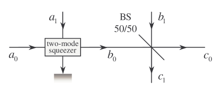
Figure 7.4: Scheme of local $1$ to $2$ cloning.

Now, considering vacuum inputs for modes $a_{1}$ and $b_{1}$, and squeezing parameters $\mu=\sqrt{2}$, $\nu=1$, it follows that $\langle c_{0}\rangle=\langle c_{1}\rangle=\langle a_{0}\rangle$. As a consequence, the scheme considered allows to copy the amplitude of the original mode $a_{0}$. Thus, if the latter is excited in a coherent state two clones are produced at the output modes $c_{0}$ and $c_{1}$. The optimality of the cloner follows from the fact that the two-mode squeezing chosen yields an excess noise variance $\sigma^{2}=1/2$ [163]. Finally, the generalization of this method allows to realize an optimal $n$ to $m$ local cloning machine.

7.2.2 Telecloning

The cloning process described above, even if local, may be applied in order to distribute quantum information among many distant parties, in what is called a quantum information network. Suppose that one wants to distribute the information stored into $n$ states to $m$ receivers. This may be achieved by two steps. One may first produce locally $m$ copies of the original states by means of the cloning protocol presented above. Then, the teleportation of each copy, following the scheme described in Section 7.1, allows to attain the transfer of information [164]. This strategy has the obvious advantage to use only bipartite entangled sources. However, even in the absence of losses, it does not leave the receivers with $m$ optimum clones of the original states, due to the non-unitary fidelity of the teleportation protocol in case of finite energy. This problem may be circumvented by pursuing a one-step strategy consisted of a nonlocal cloning. By this we mean that the cloning process is supported by a multipartite ($m+n$) entangled state which is distributed among all the parties involved. This so called telecloning process is thus nonlocal in the sense that it proceed along the lines of a natural generalization of the teleportation protocol to the many-recipient case [164]. To clarify this second scenario, let us describe now in details a $1$ to $2$ telecloning process based on the tripartite state $|T\rangle$ introduced in Eq. (2.49) [47].

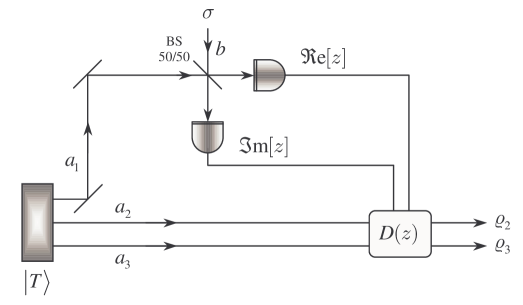
Figure 7.5: Schematic diagram of the $1\rightarrow 2$ telecloning scheme described in the text.

A schematic diagram of the telecloning process is depicted in Fig. 7.5. After the preparation of the state $|T\rangle$, a joint measurement is made on the mode $a_{1}$ and the mode $b$ to be telecloned, which corresponds to the measure of the complex photocurrent $Z=b+a_{1}^{\dagger}$, as in the case of the teleportation protocol. The whole measurement is described by the POVM (5.122), acting on the mode $a_{1}$, namely $\Pi(z)=\pi^{-1}D(z)\>\sigma^{\scriptscriptstyle T}D^{\dagger}(z)$, where $\sigma$ is the the state to be teleported and cloned. The probability distribution of the outcomes is given by

$$P(z) =\hbox{Tr}_{123}\left[|T\rangle\langle T|\>\Pi(z)\otimes\mathbb{I}_{2}\otimes\mathbb{I}_{3}\right]$$

$$=\frac{1}{\pi(1+N_{1})}\sum_{pq}\frac{N_{2}^{p}N_{3}^{q}}{(1+N_{1})^{p+q}}\frac{(p+q)!}{p!\>q!}\>\langle p+q|D(z)\,\sigma^{\scriptscriptstyle T}D^{\dagger}(z)|p+q\rangle\;.$$ (7.63)

The conditional state of the mode $a_{2}$ and $a_{3}$ after the outcome $z$ is given by

$$\varrho_{z} =\frac{1}{P(z)}\>\hbox{Tr}_{1}\left[|T\rangle\langle T|\>\Pi(z)\otimes\mathbb{I}_{2}\otimes\mathbb{I}_{3}\right]$$

$$=\frac{1}{P(z)}\frac{1}{\pi(1+N_{1})}\sum_{p,q}\sum_{k,l}\sqrt{\frac{N_{2}^{p+k}\,N_{3}^{q+l}}{(1+N_{1})^{p+q+k+l}}}\,\sqrt{\frac{(p+q)!}{p!\,q!}\frac{(k+l)!}{k!\,l!}}\,$$

$$\hskip 128.0374pt\times\langle k+l|D(z)\,\sigma^{\scriptscriptstyle T}D^{\dagger}(z)|p+q\rangle\>|p,q\rangle\langle k,l|\;.$$ (7.64)

After the measurement, the conditional state should be transformed by a further unitary operation, depending on the outcome of the measurement. In our case, this is a two-mode product displacement $U_{z}=D_{2}^{\scriptscriptstyle T}(z)\otimes D_{3}^{\scriptscriptstyle T}(z)$. This is a local transformation which generalizes to two modes the procedure already used in the original CVQT protocol described in Section 7.1. The overall state of the two modes is obtained by averaging over the possible outcomes

$$\varrho_{23}=\int_{\mathbb{C}}d^{2}z\>P(z)\>\tau_{z}\>.$$

where $\tau_{z}=U_{z}\>\varrho_{z}\>U_{z}^{\dagger}$.

If $b$ is excited in a coherent state $\sigma=|\alpha\rangle\langle\alpha|$, then the probability of the outcomes is given by

$$P_{\alpha}(z)=\frac{1}{\pi(1+N_{1})}\>\exp\left\{-\frac{|z+\alpha^{*}|^{2}}{1+N_{1}}\right\}\;.$$ (7.65)

Moreover, since the POVM is pure also the conditional state is pure. Is this way we have that $\varrho_{z}=|\psi_{z}\rangle\rangle\langle\langle\psi_{z}|$ is the product of two states, namely

$$|\psi_{z}\rangle\rangle=|(\alpha+z^{*})\,\varepsilon_{2}\rangle\otimes|(\alpha+z^{*})\,\varepsilon_{3}\rangle\;,$$ (7.66)

where

$$\varepsilon_{h}=\sqrt{\frac{N_{h}}{1+N_{1}}}\qquad(h=2,3)\;.$$ (7.67)

Correspondingly, we have $\tau_{z}=U_{z}\>|\psi_{z}\rangle\rangle\langle\langle\psi_{z}|\>U_{z}^{\dagger}$ with

$$U_{z}\>|\psi_{z}\rangle\rangle=|\alpha\varepsilon_{2}+z^{*}\,(\varepsilon_{2}-1)\rangle\otimes|\alpha\varepsilon_{3}+z^{*}\,(\varepsilon_{3}-1)\rangle\>.$$ (7.68)

The partial traces $\varrho_{2}=\hbox{Tr}_{3}[\varrho_{23}]$ and $\varrho_{3}=\hbox{Tr}_{2}[\varrho_{23}]$ read as follows

$$\varrho_{h}=\int_{\mathbb{C}}d^{2}z\>P_{\alpha}(z)\>|\alpha\varepsilon_{h}+z^{*}\,(\varepsilon_{h}-1)\rangle\langle\alpha\varepsilon_{h}+z^{*}\,(\varepsilon_{h}-1)|\;.$$ (7.69)

From the teleported states in (7.69) we see that, depending on the values of the coupling constants of the Hamiltonian (2.48) the two clones can either be equal one to each other or be different. In other words, a remarkable feature of this scheme is that it is suitable to realize both symmetric, when $N_{2}=N_{3}=N$, and asymmetric cloning, $N_{2}\neq N_{3}$. This arise as a consequence of the possible asymmetry of the state that supports the teleportation.

Let us first consider the symmetric cloning. According to Eq. (2.50) the condition $N_{2}=N_{3}=N$ holds when

$$\cos(\Omega t)=\frac{|\gamma_{1}|^{2}}{2|\gamma_{2}|^{2}-|\gamma_{1}|^{2}}\;,\qquad N=\frac{4|\gamma_{1}|^{2}|\gamma_{2}|^{2}}{(2|\gamma_{2}|^{2}-|\gamma_{1}|^{2})^{2}}\;.$$ (7.70)

Since $|\langle z^{{}^{\prime}}|z^{{}^{\prime\prime}}\rangle|^{2}=\exp\{-|z^{{}^{\prime}}-z^{{}^{\prime\prime}}|^{2}\}$, the fidelity of the clones is given by (we put $\varepsilon_{2}=\varepsilon_{3}=\varepsilon$)

$$F =\int_{\mathbb{C}}\frac{d^{2}z}{\pi(2N+1)}\>\exp\left\{-\frac{|\alpha+z^{*}|^{2}}{2N+1}\right\}\>\exp\left\{-|\alpha+z^{*}|^{2}(\varepsilon-1)^{2}\right\}$$

$$=\left(2+3N-2\sqrt{N(2N+1)}\right)^{-1}\;.$$ (7.71)

As we expect from a proper cloning machine, the fidelity is independent of the amplitude of the initial signal and for $0<N<4$ it is larger than the classical limit $F=1/2$. Notice that the transformation $U_{z}$ performed after the conditional measurement, is the only one assuring that the output fidelity is independent of the amplitude of the initial state. Exploiting Eq. (7.71) we can see that the fidelity reaches its maximum $F=2/3$ for $N=1/2$ which means, according to Eq. (7.70), that the physical system allows an optimal cloning when its coupling constants are chosen in such a way that $|\gamma_{1}/\gamma_{2}|=(6-\sqrt{32})^{1/2}\simeq 0.586$ . The total mean photon number required to reach the optimal telecloning is thus $N_{1}+N_{2}+N_{3}=2$, hence, as we claimed above, it can be achieved without the need of infinite energy. The scheme presented is analog to that of Ref. [125] in the absence of an amplification process for the signal. There, the telecloning is supported by a state similar to the one given in Eq. (2.46), where at the input ports of the tritter only two squeezed states are involved, the third mode being a vacuum state. Both the protocols described here and in Ref. [125] achieve the optimality relying on minimal energetic resources, i.e. the total mean photon number is $2$ in both cases. Notice that a generalization to realize a $1\rightarrow m$ telecloning machine can be realized upon the implementation of ${\rm SU}(p,1)$ Hamiltonian introduced in Section 1.4.5. In fact, having at disposal a $1+m$ multipartite entangled state of the form (1.126), it is straightforward to show that a measurement of $Z$ on the mode to be telecloned and the sum-mode of (1.126), followed by a local multimode displacement operation provides optimal clones in the remaining $m$ modes.

Let us now consider the asymmetric case. For $N_{2}\neq N_{3}$ the fidelities of the two clones (7.69) are given by

$$F_{h}=\left(2+N_{h}+2N_{k}-2\sqrt{N_{h}(N_{1}+1)}\right)^{-1}\;,$$ (7.72)

where $h,k=2,3$ ($h\neq k$). A question arises whether it is possible to tune the coupling constants so as to obtain a fidelity larger than the bound $F=2/3$ for one of the clones, say $\varrho_{2}$, while accepting a decreased fidelity for the other clone. In particular if we impose $F_{3}=1/2$, i.e. the minimum value to assure the genuine quantum nature of the telecloning protocol, we can maximize $F_{2}$ by varying the value of the coupling constants $\gamma_{1}$ and $\gamma_{2}$. The maximum value turns out to be $F_{2,{\rm max}}=4/5$ and it corresponds to the choice $N_{3}=1/4$ and $N_{2}=1$. More generally one can fix $F_{3}$, then the maximum value of $F_{2}$ is obtained choosing $N_{2}=(1/F_{3}-1)$ and $N_{3}=(4/F_{3}-4)^{-1}$. The relation between the fidelities is then

$$F_{2}=4\frac{(1-F_{3})}{(4-3F_{3})}\>,$$ (7.73)

which shows that $F_{2}$ is a decreasing function of $F_{3}$ and that $2/3<F_{2}<4/5$ when $1/2<F_{3}<2/3$ . The sum of the two fidelities $F_{2}+F_{3}=1+3F_{2}F_{3}/4$ is maximized in the symmetric case in which optimal fidelity $F_{2}=F_{3}=2/3$ can be reached. The role of $\varrho_{2}$ and $\varrho_{3}$ can be exchanged, and the above considerations still hold.

Chapter 8 State engineering

In this Chapter we analyze the use of conditional measurements on entangled twin-beam state (TWB) of radiation to engineer quantum states, i.e. to produce, manipulate, and transmit nonclassical light. In particular, we will focus our attention on realistic measurement schemes, feasible with current technology, and will take into account imperfections of the apparata such as quantum efficiency and finite resolution.

The reason to choose TWB as entangled resource for conditional measurements is twofold. On one hand, TWBs are the natural generalization to continuous variable (CV) systems of Bell states, i.e. maximally entangled states for qubit systems. On the other hand TWBs are CV entangled states that can be reliably produced with current technology, either by parametric downconversion of the vacuum in a nondegenerate parametric amplifier [165], or by mixing two squeezed vacua from a couple of degenerate parametric amplifiers in a balanced beam splitter [27, 26].

The first kind of measurement we analyze is on/off photodetection, which provides the generation of conditional nonclassical mixtures, which are not destroyed by decoherence induced by noise and permits a robust test of the quantum nature of light.

The second apparatus is homodyne detection, which represents a tunable source of squeezed light, with high conditional probability and robustness to experimental imperfections, such non-unit quantum efficiency and finite resolution.

The third kind of measurement is that of the normal operator $Z=b+c^{\dagger}$, $b$ and $c$ being two modes of the field, as described in Section 5.6. In our case one of the two modes is a beam of the TWB, whereas the second one, usually referred to as the probe of the measurement, is excited in a given reference state. This approach allows to describe CV quantum teleportation as a conditional measurement, and to easily evaluate the degrading effects of finite amount of entanglement, decoherence due to losses, and imperfect detection [96].

8.1 Conditional quantum state engineering

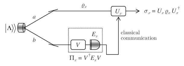
Figure 8.1: Scheme for quantum state engineering assisted by entanglement.

The general measurement scheme we are going to consider is schematically depicted in Fig. 8.1. The entangled state subjected to the conditional measurement is the TWB $|\Lambda\rangle\rangle$, $\Lambda=\sqrt{1-\lambda^{2}}\lambda^{a^{\dagger}a}$, with $\lambda=\tanh r$ assumed as real. A measurement, performed on one of the two modes, reduces the other one accordingly to the projection postulate. Each possible outcome $x$ of such a measurement occurs with probability $P_{x}$, and corresponds to a conditional state $\sigma_{x}$ on the other subsystem (Fig. 8.1). Upon denoting by $\Pi_{x}$ the POVM of the measurement we have

$$P_{x} =\hbox{Tr}_{ab}\Big{[}|\Lambda\rangle\rangle\langle\langle\Lambda|\>\mathbb{I}\otimes\Pi_{x}\Big{]}(1-\lambda^{2})\sum_{q=0}^{\infty}\>\lambda^{2q}\>\langle q|\Pi_{x}|q\rangle=(1-\lambda^{2})\,\hbox{Tr}_{b}\big{[}\lambda^{2b^{\dagger}b}\>\Pi_{x}^{\scriptscriptstyle T}\big{]}\,,$$ (8.1)

and

$$\varrho_{x} =\frac{1}{P_{x}}\,\hbox{Tr}_{b}\Big{[}|\Lambda\rangle\rangle\langle\langle\Lambda|\>\mathbb{I}\otimes\Pi_{x}\Big{]}\frac{1-\lambda^{2}}{P_{x}}\sum_{p,q}\>\lambda^{p+q}\>\langle p|\Pi_{x}^{\scriptscriptstyle T}|q\rangle\>|p\rangle\langle q|=\frac{\displaystyle\lambda^{a^{\dagger}a}\>\Pi_{x}^{\scriptscriptstyle T}\>\lambda^{a^{\dagger}a}}{\displaystyle\hbox{Tr}_{b}\big{[}\lambda^{2b^{\dagger}b}\>\Pi_{x}^{\scriptscriptstyle T}\big{]}}\,.$$ (8.2)

Notice that in the second line of Eq. (8.2) $\Pi_{x}$ should be meant as an operator acting on the Hilbert space ${\cal H}_{a}$ of the mode $a$. Our scheme is general enough to include the possibility of performing any unitary operation on the beam subjected to the measurement. In fact, if $E_{x}$ is the original POVM and $V$ the unitary, the overall measurement process is described by $\Pi_{x}=V^{\dagger}E_{x}V$, which is again a POVM. In the following we always consider $V=\mathbb{I}$, i.e. no transformation before the measurement. A further generalization consists in sending the result of the measurement (by classical communication) to the reduced state location and then performing a conditional unitary operation $U_{x}$ on the conditional state, eventually leading to the state $\sigma_{x}=U_{x}\varrho_{x}U_{x}^{\dagger}$. This degree of freedom will be used in Section 8.1.3, where we re-analyze CV quantum teleportation as a conditional measurement.

8.1.1 On/off photodetection

By looking at the expression of TWB in the Fock basis, $|\Lambda\rangle\rangle=\sqrt{1-\lambda^{2}}\sum_{q}\lambda^{q}|q\rangle|q\rangle$, or at Eq. (8.2) it is apparent that ideal photocounting on one of the two beams, described by the POVM $\Pi_{k}=|k\rangle\langle k|$, is a conditional source of Fock number state $|k\rangle$, which would be produced with a conditional probability $P_{k}=(1-\lambda^{2})\lambda^{k}$. However, realistic photocounting can be very challenging experimentally, therefore we consider the situation in which one of the two beams, say mode $b$, is revealed by an avalanche on/off photodetector (see Section 5.3.2). The action of an on/off detector is described by the two-value POVM $\{\Pi_{0}(\eta),\Pi_{1}(\eta)\}$ given in Eq. (5.20). The outcome “$1$” (i.e. registering a “click” corresponding to one or more incoming photons) occurs with probability

$$P_{1}=\langle\langle\Lambda|\mathbb{I}\otimes\Pi_{1}(\eta)|\Lambda\rangle\rangle=\frac{\eta\,\lambda^{2}}{1-\lambda^{2}(1-\eta)}=\frac{\eta\,N_{\lambda}}{2+\eta\,N_{\lambda}}\;,$$ (8.3)

with $N_{\lambda}=2\lambda^{2}/(1-\lambda^{2})$, and correspondingly, the conditional output state for the mode $a$ is given by [166]

$$\varrho_{1}=\frac{1-\lambda^{2}}{P_{1}}\sum_{k=1}^{\infty}\lambda^{2k}\left[1-(1-\eta)^{k}\right]\>|k\rangle\langle k|\;.$$ (8.4)

The density matrix in Eq. (8.4) describes a mixture: a pseudo-thermal state where the vacuum component has been removed by the conditional measurement. Such a state is highly nonclassical, as also discussed in Ref. [8]. Notice that the nonclassicality is present only when the state exiting the amplifier is entangled. In the limit of low TWB energy the conditional state $\varrho_{1}$ approaches the number state $|1\rangle\langle 1|$ with one photon.

The Wigner function $W[\varrho_{1}](\alpha)$ of $\varrho_{1}$ exhibits negative values for any value of $\lambda$ and $\eta$. In particular, in the origin of the phase space we have

$$W[\varrho_{1}](0)=-\frac{2}{\pi}\>\frac{1}{1+N_{\lambda}}\>\frac{2+\eta\,N_{\lambda}}{2(1+N_{\lambda})-\eta\,N_{\lambda}}\;.$$ (8.5)

One can see that also the generalized Wigner function for $s$-ordering

$$W_{s}[\varrho_{1}](\alpha)=-\frac{2}{\pi s}\int_{\mathbb{C}}d^{2}\gamma\>W[\varrho_{1}](\gamma)\,\exp\left\{\>-\frac{2}{s}\>|\alpha-\gamma|^{2}\right\}\>,$$

shows negative values for $s\in(-1,0)$. In particular one has

$$W_{s}[\varrho_{1}](0)=-\frac{2(1+s)(2+\eta\,N_{\lambda})}{\pi(1+N_{\lambda}-s)\left[2(1+N_{\lambda}-s)-\eta\,N_{\lambda}(1+s)\right]}\;.$$ (8.6)

A good measure of nonclassicality is given by the lowest index $s^{\star}$ for which $W_{s}$ is a well-behaved probability, i.e. regular and positive definite [83]. Eq. (8.6) says that for $\varrho_{1}$ we have $s^{\star}=-1$, that is $\varrho_{1}$ describes a state as nonclassical as a Fock number state.

Since the Fano factor of $\varrho_{1}$ is given by

$$F\equiv\frac{\left\langle[b^{\dagger}b-\langle b^{\dagger}b\rangle]^{2}\right\rangle}{\langle b^{\dagger}b\rangle}=\frac{\left(2+N_{\lambda}\right)}{2}\left[1+{\frac{2}{2+\eta\,N_{\lambda}}}-{\frac{4\,\left(2+N_{\lambda}\right)}{4+N_{\lambda}\,\left(4+\eta\,N_{\lambda}\right)}}\right]\;,$$ (8.7)

we have that the beam $b$ is always subPossonian for (at least) $N_{\lambda}<2$. The verification of nonclassicality can be performed, for any value of the gain, by checking the negativity of the Wigner function through quantum homodyne tomography [166], and in the low gain regime, also by verifying the subPoissonian character by measuring the Fano factor via direct noise detection [167, 168].

Note that besides quantum efficiency, i.e. lost photons, the performance of a realistic photodetector may be degraded by the presence of dark-counts, i.e. by “clicks” that do not correspond to any incoming photon. In order to take into account both these effects we should describe the detector by the POVM (5.22) rather than (5.20). However, at optical frequencies the number of dark counts is small and we are not going here to take into account this effect, which have been analyzed in details in Ref. [166].

8.1.2 Homodyne detection

In this Section we consider the kind of conditional state that can be obtained by homodyne detection on one of the two beams of the TWB . We will show that they are squeezed states. We first consider ideal homodyne detection described by the POVM $\Pi_{x}=|x\rangle\langle x|$ where $|x\rangle$ denotes the eigenstate (1.15) of the quadratures $x=\frac{1}{2}(a+a^{\dagger})$ (throughout the Section we use $\kappa_{1}=\kappa_{2}=1$) and where, without loss of generality, we have chosen a zero reference phase (see Section 5.5 for details about homodyne detection). Then, in the second part of the Section we will consider two kinds of imperfections: non-unit quantum efficiency and finite resolution. As we will see, the main effect of the conditional measurement, i.e the generation of squeezing, holds also for these realistic scenarios.

The probability of obtaining the outcome $x$ from a homodyne detection on the mode $b$ is obtained from Eq. (8.1). We have

$$P_{x}=(1-\lambda)^{2}\sum_{q=0}^{\infty}\lambda^{2q}\>\left|\langle x|q\rangle\right|^{2}=\frac{1}{\sqrt{2\pi\sigma_{\lambda}^{2}}}\ \exp\left\{-\frac{x^{2}}{2\sigma_{\lambda}^{2}}\right\}\;,$$ (8.8)

where

$$\sigma_{\lambda}^{2}=\frac{1}{4}\frac{1+\lambda^{2}}{1-\lambda^{2}}=\frac{1}{4}(1+N_{\lambda})\>.$$ (8.9)

$P_{x}$ is Gaussian with variance that increases as $\lambda$ is approaching unit. In the (unphysical) limit $\lambda\rightarrow 1$, i.e. infinite gain of the amplifier, the distribution for $x$ is uniform over the real axis. The conditional output state is given by Eq. (8.2), and, since $\Pi_{x}$ is a pure POVM, it is a pure state $\varrho_{x}=|\psi_{x}\rangle\langle\psi_{x}|$ where

$$|\psi_{x}\rangle=\sqrt{\frac{1-\lambda^{2}}{P_{x}}}\,\lambda^{a^{\dagger}a}\>|x\rangle=\sum_{k=0}^{\infty}\psi_{k}\,|k\rangle\;.$$ (8.10)

The coefficients of $|\psi_{x}\rangle$ in the Fock basis are given by

$$\psi_{k}=(1-\lambda^{4})^{1/4}\left(\frac{\lambda^{2}}{2}\right)^{k/2}\frac{H_{k}(\sqrt{2}x)}{\sqrt{k!}}\,\exp\left\{-\frac{2\lambda^{2}x^{2}}{1+\lambda^{2}}\right\}\,,$$ (8.11)

which means that $|\psi_{x}\rangle$ is a squeezed state of the form

$$|\psi_{x}\rangle=D(\alpha_{x})S(\zeta)|0\rangle\>,$$ (8.12)

where

$$\alpha_{x} =\frac{2x\lambda}{1+\lambda^{2}}=\frac{x\sqrt{N_{\lambda}(N_{\lambda}+2)}}{1+N_{\lambda}}$$ (8.13a)

$$\zeta =\tanh^{-1}(\lambda^{2})=\tanh^{-1}\left(\frac{N_{\lambda}}{N_{\lambda}+2}\right)\>,$$ (8.13b)

and the quadrature fluctuations are given by

$$\Delta x_{a}^{2}=\frac{1}{4}\frac{1}{1+N_{\lambda}}\,,\qquad\Delta y_{a}^{2}=\frac{1}{4}(1+N_{\lambda})\>.$$ (8.14)

Notice that (i) the amount of squeezing is independent on the outcome of the measurement, which only influences the coherent amplitude; (ii) according to Eq. (8.8) the most probable conditional state is a squeezed vacuum. The average number of photon of the conditional state is given by

$$N_{x}=\langle\psi_{x}|a^{\dagger}a|\psi_{x}\rangle=x^{2}\,\frac{N_{\lambda}(2+N_{\lambda})}{(1+N_{\lambda})^{2}}+\frac{1}{4}\,\frac{N_{\lambda}^{2}}{1+N_{\lambda}}\>.$$ (8.15)

The conservation of energy may be explicitly checked by averaging over the possible outcomes, namely

$$\int_{\mathbb{R}}dx\>P_{x}\>N_{x}=\frac{1}{4}\frac{N_{\lambda}^{2}}{1+N_{\lambda}}+\sigma_{\lambda}^{2}\,\frac{N_{\lambda}(2+N_{\lambda})}{(1+N_{\lambda})^{2}}=\frac{1}{2}\,N_{\lambda}\>,$$ (8.16)

which correctly reproduces the number of photon pertaining each part of the TWB.

We now take into account the effects of non-unit quantum efficiency $\eta$ at the homodyne detector on the conditional state. We anticipate that $\varrho_{x\eta}$ will be no longer pure states, and in particular they will not be squeezed states of the form (8.12). Nevertheless, the conditional output states still exhibit squeezing, i.e. quadrature fluctuations below the coherent level, for any value of the outcome $x$, and for $\eta>1/2$. The POVM of a homodyne detector with quantum efficiency $\eta$ is given in Eq. (5.67). Since the nonideal POVM is a Gaussian convolution of the ideal POVM, the main effect is that $\Pi_{x\eta}$ is no longer a pure orthogonal POVM. The probability $P_{x\eta}$ of obtaining the outcome $x$ is still a Gaussian with variance

$$\Delta^{2}_{\lambda\eta}=\sigma_{\lambda}^{2}+\delta_{\eta}^{2}\>,$$ (8.17)

where $\delta_{\eta}^{2}$ is given in Eq. (5.68). The conditional output state is again given by Eq. (8.2). After some algebra we get the matrix element in the Fock basis

$$\langle n|\varrho_{x\eta}|m\rangle=\frac{\left(1-\lambda^{2}\right)\lambda^{n+m}}{\sqrt{2^{n+m}n!m!}}\sqrt{\frac{\eta\,[2-\eta(1-\lambda^{2})]}{1-\lambda^{2}}}\exp\left\{-\frac{4\eta^{2}\lambda^{2}x^{2}}{1-\lambda^{2}(1-2\eta)}\right\}\\ \times\sum_{k=0}^{{\rm min}[m,n]}\!\!\!2^{k}k{m\choose k}{n\choose k}\,\sqrt{\eta^{m+n-2k}}\,H_{m+n-2k}\left(\sqrt{2\eta}\>x\right)\>,$$ (8.18)

where $H_{n}(x)$ is the $n$-th Hermite polynomials. The quadrature fluctuations are now given by

$$\Delta x_{a}^{2}=\frac{1}{4}\frac{1+N_{\lambda}(1-\eta)}{1+\eta\,N_{\lambda}}\,,\qquad\Delta y_{a}^{2}=\frac{1}{4}(1+N_{\lambda})\>.$$ (8.19)

As a matter of fact, $\Delta y_{a}^{2}$ is independent on $\eta$, whereas $\Delta x_{a}^{2}$ increases for decreasing $\eta$. Therefore, the conditional output $\varrho_{x\eta}$ is no longer a minimum uncertainty state. However, for $\eta$ large enough we still observe squeezing in the direction individuated by the measured quadrature. We have that the conditional state is a general Gaussian state of the form (2.15) with an average number of thermal photons given by

$$N_{\rm th}=\frac{1}{2}\left\{\sqrt{\frac{(1+N_{\lambda})[1+N_{\lambda}(1-\eta)]}{1+\eta\,N_{\lambda}}}-1\right\}\;,$$ (8.20)

and with amplitude and squeezing parameters

$$\alpha_{x\eta}=\frac{\eta\sqrt{N_{\lambda}(N_{\lambda}+2)}}{1+\eta\,N_{\lambda}}\>x\,,\qquad\xi_{\eta}=\frac{1}{4}\ln\left[\frac{(1+N_{\lambda})(1+\eta\,N_{\lambda})}{1+N_{\lambda}(1-\eta)}\right]\;.$$ (8.21)

From Eqs. (8.19) and (8.21) we notice that $\varrho_{x\eta}$ shows squeezing if $\eta>1/2$, independently on the actual value $x$ of the homodyne outcome.

The outcome of homodyne detection is, in principle, continuously distributed over the real axis. However, in practice, one has always to discretize data, mostly because of finite experimental resolution. The POVM describing homodyne detection with binned data is given by

$$\Pi_{x\eta}(\delta)=\frac{1}{\delta}\int_{x-\delta/2}^{x+\delta/2}dt\>\Pi_{t\eta}\;,$$ (8.22)

where $\Pi_{t\eta}$ is given in Eq. (5.67), and $\delta$ is the width of the bins. The probability distribution is now given by

$$P_{x\eta}(\delta) =\frac{1}{2\delta}\left[\hbox{Erf}\left(\frac{x+\mbox{$\frac{1}{2}$}\delta}{\sqrt{2\Delta^{2}_{\lambda\eta}}}\right)-\hbox{Erf}\left(\frac{x-\mbox{$\frac{1}{2}$}\delta}{\sqrt{2\Delta^{2}_{\lambda\eta}}}\right)\right]$$ (8.23)

$$=\frac{1}{\sqrt{2\pi\Delta^{2}_{\lambda\eta}}}\,\exp\left\{-\frac{x^{2}}{2\Delta^{2}_{\lambda\eta}}\right\}\,\left(1-\frac{x^{2}-\Delta^{2}_{\lambda\eta}}{24\Delta^{2}_{\lambda\eta}}\>\delta^{2}\right)+O(\delta^{3})\;$$ (8.24)

where $\Delta_{\lambda\eta}^{2}$ is given in Eq. (8.17) and

$$\hbox{Erf}(x)=\frac{2}{\sqrt{\pi}}\int_{0}^{x}dt\,e^{-t^{2}}$$

denotes the error function. The conditional state is modified accordingly. Concerning the quadrature fluctuations of the conditional state we have, up to second order in $\delta$,

$$\Delta x_{a}^{2}(\delta)=\Delta x_{a}^{2}+\frac{\delta^{2}}{12}\frac{\eta^{2}N_{\lambda}(2+N_{\lambda})}{(1+\eta\,N_{\lambda})^{2}}\,x^{2}\;,$$ (8.25)

which is below the coherent level for $\eta>1/2$ and for

$$|x|<x_{\delta}\equiv\frac{1}{\delta}\sqrt{\frac{3(1+\eta\,N_{\lambda})(2\eta-1)}{\eta^{2}(N_{\lambda}+2)}}\;.$$ (8.26)

Therefore, the effect of finite resolution is that the conditional output is squeezed only for the subset $|x|<x_{\delta}$ of the possible outcomes which, however, represents the range where the probability is higher [96].

8.1.3 Joint measurement of two-mode quadratures

In this Section we assume that mode $b$ is subjected to the measurement of the the real and the imaginary part of the complex operator $Z=b+c^{\dagger}$, where $c$ is an additional mode excited in a reference state $S$. As we have seen in Section 5.6 this kind of measurement is described by the POVM

$${\Pi}_{\alpha}=\frac{1}{\pi}{D}(\alpha)\,{S}^{\scriptscriptstyle T}\,{D}^{{\dagger}}(\alpha)\>.$$ (8.27)

The present scheme is equivalent to that of CV teleportation, which, as pointed out in Section 7.1.1, can be viewed as a conditional measurement, with the state to be teleported playing the role of the reference state $S$ of the apparatus. In order to complete the analogy we assume that the result of the measurement is classically transmitted to the receiver’s location, and that a displacement operation $D^{\dagger}(\alpha)$ is performed on the conditional state $\varrho_{\alpha}$. Eqs. (8.1) and (8.2) are rewritten as follows

$$p_{\alpha} =(1-\lambda^{2})\hbox{Tr}^{2}\left[\lambda^{2a^{\dagger}a}\>\Pi_{\alpha}^{\scriptscriptstyle T}\right]$$ (8.28)

$$\varrho_{\alpha} =\frac{\displaystyle\lambda^{a^{\dagger}a}\>\Pi_{\alpha}^{\scriptscriptstyle T}\>\lambda^{a^{\dagger}a}}{\displaystyle\hbox{Tr}^{2}\left[\lambda^{2a^{\dagger}a}\>\Pi_{\alpha}^{\scriptscriptstyle T}\right]}$$ (8.29)

$$\sigma_{\alpha} =D^{{\dagger}}(\alpha)\,\varrho_{\alpha}\,D(\alpha)=\frac{D^{\dagger}(\alpha)\lambda^{a^{\dagger}a}\>D(\alpha)\,S\,D^{\dagger}(\alpha)\>\lambda^{a^{\dagger}a}D(\alpha)}{\displaystyle\hbox{Tr}^{2}\left[\lambda^{2a^{\dagger}a}\>\Pi_{\alpha}^{\scriptscriptstyle T}\right]}\;,$$ (8.30)

while the teleported state is the average over all the possible outcomes, i.e.

$$\sigma=\int_{\mathbb{C}}d^{2}\alpha\,p_{\alpha}\,\sigma_{\alpha}=\int_{\mathbb{C}}d^{2}\alpha\,D^{\dagger}(\alpha)\,\langle\langle\Lambda|\mathbb{I}\otimes\Pi_{\alpha}|\Lambda\rangle\rangle\,D(\alpha)\;.$$ (8.31)

After performing the partial trace, and some algebra, one has

$$\sigma=\int_{\mathbb{C}}\frac{d^{2}\alpha}{\pi\sigma_{-}^{2}}\,\exp\left\{-\frac{|\alpha|^{2}}{\sigma_{-}^{2}}\right\}\,D(\alpha)SD^{{\dagger}}(\alpha)\;,$$ (8.32)

where $\sigma_{-}^{2}=1+N_{\lambda}-\sqrt{N_{\lambda}(N_{\lambda}+2)}$, i.e. the result of Section 7.1.

Bibliography

- [1] S. L. Braunstein, P. van Loock, quant-ph/0410100, Rev. Mod. Phys., in press.
- [2] J. Eisert, M.B. Plenio, Int. J. Quant. Inf. 1, 479 (2003).
- [3] R. Simon, E. C. G. Sudarshan, and N. Mukunda, Phys. Rev. A 36, 3868 (1987); R. Simon, N. Mukunda, and B. Dutta, Phys. Rev. A 49, 1567 (1994).
- [4] P. Lo Presti, Nuove misurazioni quantistiche, Tesi di Laurea Università di Pavia, a.a. 1998/1999; G. M. D’Ariano, P. Lo Presti, and M. F. Sacchi, Phys. Lett. A 272, 32 (2000).
- [5] R. Littlejohn, Phys. Rep. 138, 193 (1986).
- [6] R. Simon, E. C. G. Sudarshan, and N. Mukunda, Phys. Rev. A 37, 3028 (1988); Arvind, B. Dutta, N. Mukunda, and R. Simon, Pramana-Journ. Phys. 45, 471 (1995) (e-print quant-ph/9509002).
- [7] A Wunschë, J. Opt. B 4, 1 (2002).
- [8] L. Mandel, E. Wolf, Optical Coherence and Quantum Optics, (Cambridge Univ. Press, 1995)
- [9] D. N. Klysko, Photons and Non-Linear Optics, (Gordon and Breach, Amsterdam, 1988), originally published as Fotony i nelineinaya optika, (Nauka, Moscow, 1980)
- [10] P. Meystre, Atom Optics, Springer Series on Atomic Phys., 33 (Springer, Berlin, 2001).
- [11] N. Piovella, M. Cola, and R. Bonifacio, Phys. Rev. A 67, 013817 (2003).
- [12] M. G. A. Paris, M. Cola, N. Piovella, and R. Bonifacio, Opt. Comm. 227, 349 (2003); M. M. Cola, M. G. A. Paris, N. Piovella, and R. Bonifacio, J. Phys. B 37, 187 (2004).
- [13] M. M. Cola, M. G. A. Paris, and N. Piovella, Phys. Rev. A 70, 043809 (2004).
- [14] L. M. Kuang LM, A. H. Zeng AH, and Z. H. Kuang, Phys. Lett. A 319, 24 (2003).
- [15] S. L. Braunstein, e-print quant-ph/9904002.
- [16] R. J. Glauber, Phys. Rev. A 131, 2766 (1963); K. Cahill, and R. Glauber, Phys. Rev. 177, 1857 (1969); ibid. 1882 (1969).
- [17] G. M. D’Ariano, and M. F. Sacchi, Phys. Rev. A 52, R4309 (1995).
- [18] J. Schwinger in Quantum Theory of Angular Momentum, L. C. Biedenharn and H. Van Dam (Eds.), (New York, Academic Press, 1965), pp. 274-276.
- [19] W. Magnus, Commun. Pure Appl. Math. 7, 649 (1954).
- [20] R. M. Wilcox, J. Math. Phys. 8, 962 (1967).
- [21] W. Witschel, J. Phys. A 8, 143 (1975).
- [22] J. Fröhlich, Comm. Math. Phys. 54, 135 (1977).
- [23] H. P. Yuen, Phys. Rev. A 13, 2226 (1976).
- [24] M. S. Kim, F. A. M. de Oliveira, and P. L. Knight, Phys. Rev. A 40, 2494 (1989).
- [25] P. Marian, Phys. Rev. A 45 2044 (1992); P. Marian, and T. A. Marian, Phys. Rev. A 47, 4474 (1993); ibid. 4487 (1993).
- [26] M. G. A. Paris, Phys. Lett. A 225, 28 (1997).
- [27] A. Furusawa, J. L. Sorensen, S. L. Braunstein, C. A. Fuchs, H. J. Kimble, and E. S. Polzik, Science 282, 706 (1998).
- [28] R. R. Puri, Phys. Rev. A 50, 5309 (1994)
- [29] H. J. Carmichael, Statistical methods in quantum optics 1, (Springer, Berlin, 1999).
- [30] R. L. Hudson, Rep. Math. Phys. 6, 249 (1974).
- [31] N. Lütkenhaus, and S. M. Barnett, Phys. Rev. A 51, 3340 (1995).
- [32] S. Saks, and A. Zygmund, Analytical functions (Elsevier, Amsterdam, 1971).
- [33] J. Williamson, Am. J. of Math. 58, 141 (1936).
- [34] G. Adam, J. Mod. Opt. 42, 1311 (1995).
- [35] S. M. Barnett, and P. M. Radmore, Methods in Theoretical Quantum Optics (Clarendon Press, Oxford, 1997).
- [36] D. Walls, and G. Milburn, Quantum optics (Springer Verlag, Berlin, 1994).
- [37] V. V. Dodonov, J. Opt. B 4, S98 (2002).
- [38] G. S. Agarwal, Phys. Rev. A 3, 828 (1971).
- [39] R. A. Horne, and C. R. Johnson, Matrix Analysis (Cambridge University Press, Cambridge, 1985); F. Zhang, Matrix Theory, (Springer, Berlin Heidelberg, 1999).
- [40] A. Botero, and B. Reznik, Phys. Rev. A 67, 052311 (2003).
- [41] A. S. Holevo, and R. F. Werner, Phys. Rev. A 63, 032312 (2001).
- [42] G. Giedke, J. Eisert, J. I. Cirac, and M. B. Plenio, Quant. Inf. Comp. 3, 211 (2003).
- [43] R. Simon, Phys. Rev. Lett. 84, 2726 (2000).
- [44] A. Serafini, F. Illuminati, and S. De Siena, J. Phys. B 37, L21 (2004)
- [45] L. Wang, S. S. Li, and Y. Yan, J. Phys. A: Math. Gen. 37, 10699 (2004).
- [46] P. van Loock, and S. L. Braunstein, Phys. Rev. Lett. 84, 3482 (2003).
- [47] A. Ferraro, M. G. A. Paris, M. Bondani, A. Allevi, E. Puddu, and A. Andreoni, J. Opt. Soc. Am. B 21, 1241 (2004).
- [48] S. Pirandola, S. Mancini, D. Vitali, and P. Tombesi, Phys. Rev. A 68, 062317 (2003).
- [49] T. Aoki, N. Takei, H. Yonezawa, K. Akui, T. Hiraoka, A. Furusawa , and P. van Loock, Phys. Rev. Lett. 91, 080404 (2003); H. Yonezawa, T. Aoki, and A. Furusawa, Nature 431, 430 (2004)
- [50] M. Bondani, A. Allevi, E. Puddu, A. Andreoni, A. Ferraro, and M. G. A. Paris, Opt. Lett. 29, 180 (2004);
- [51] R. F. Werner, Phys. Rev. A 40, 4277 (1989).
- [52] S. Popescu, and D. Rohrlich, Phys. Rev. A 56, R3319 (1997).
- [53] N. Gisin, and A. Peres, Phys. Lett. A 162, 15 (1992).
- [54] A. Peres, Phys. Rev. Lett. 77, 1413 (1996).
- [55] M. Horodecki, P. Horodecki, and R. Horodecki, Phys. Lett. A 223, 1 (1996).
- [56] E. Strømer, Acta Math. 110, 223 (1963)
- [57] P. Horodecki, Phys. Lett. A, 232 (1997).
- [58] Lu-Ming Duan, G. Giedke, J. I. Cirac, and P. Zoller, Phys. Rev. Lett. 84, 2722 (2000).
- [59] G. Giedke, Quantum information and continuous variable systems, Ph.D. Dissertation (University of Innsbruck, 2001).
- [60] S. M. Tan, Phys. Rev. A 60, 2752 (1999).
- [61] V. Giovannetti, S. Mancini, D. Vitali, and P. Tombesi, Phys. Rev. A 67, 022320 (2003).
- [62] P. van Loock, and A. Furusawa, Phys. Rev. A 67, 052315 (2003).
- [63] G. M. D’Ariano, C. Macchiavello, M. G. A. Paris, Phys. Rev. A 67, 042310 (2003).
- [64] R. F. Werner, and M. M. Wolf, Phys. Rev. Lett. 86, 3658 (2001).
- [65] G. Giedke, B. Kraus, M. Lewenstein, and J. I. Cirac, Phys. Rev. Lett. 87, 167904 (2001).
- [66] A. Serafini, G. Adesso, and F. Illuminati, e-print quant-ph/0411109.
- [67] C. H. Bennett, D. P. Di Vincenzo, J. A. Smolin, and W. K. Wootters, Phys. Rev. A 54, 3824 (1996).
- [68] G. Vidal, and R. F. Werner, Phys. Rev. A 65, 032314 (2002).
- [69] W. Dür, J. I. Cirac, and R. Tarrach, Phys. Rev. Lett. 83 , 3562 (1999).
- [70] D. M .Greenberger, M. A. Horne, A. Shimony, and A. Zilinger, Am. J. Phys. 58, 1131 (1990).
- [71] W. Dür, G. Vidal, and J. I. Cirac, Phys. Rev. A 62, 062314 (2000).
- [72] J. S. Bell, Physics (Long Island City, N.Y.) 1, 195 (1964).
- [73] N. D. Mermin, Phys. Rev. Lett. 65, 1838 (1990).
- [74] D. N. Klyshko, Phys. Lett. A 172, 399 (1993).
- [75] N. Gisin, and H. Bechmann-Pasquinucci, Phys. Lett. A 246, 1 (1998).
- [76] G. Giedke, B. Kraus, M. Lewenstein, and J. I. Cirac, Phys. Rev. A 64, 052303 (2001).
- [77] A. Serafini, M. G. A. Paris, F. Illuminati, and S. De Siena, preprint ArXiV: quant-ph/0501173, submitted to J. Opt. B.
- [78] A. K. Ekert et al., Phys. Rev. Lett. 88, 217901 (2001).
- [79] R. Filip, Phys. Rev. A 65, 062320 (2002).
- [80] M. Hendrych et al., e-print quant-ph/0208091.
- [81] M. G. A. Paris, A. Serafini, F. Illuminati, S. De Siena, Phys. Rev. A 68, 012314 (2003).
- [82] A. Serafini, F. Illuminati, M. G. A. Paris, S. De Siena, Phys. Rev A 69, 022318 (2004).
- [83] C. T. Lee, Phys. Rev. A 44, R2775 (1991).
- [84] K. S. Grewal, Phys Rev A 67, 022107 (2003).
- [85] S. Olivares, M. G. A. Paris, and A. R. Rossi, Phys. Lett. A 319, 32 (2003).
- [86] J. S. Prauzner-Bechcicki, e-print quant-ph/0211114 v2.
- [87] A. R. Rossi, S. Olivares, and M. G. A. Paris, J. Mod. Opt. 51, 1057 (2004).
- [88] M. A. Naimark, Izv. Akad. Nauk SSSR Ser. Mat. 4, 227 (1940).
- [89] W. Mlak, Hilbert Spaces and Operator Theory, (Kluwer Academic, Dordrecht, 1991).
- [90] P. L. Kelley, and W. H. Kleiner, Phys. Rev. 136, 316 (1964).
- [91] W. H. Louisell, Quantum Statistical properties of Radiation, (Wiley, 1973).
- [92] S. Olivares, M. G. A. Paris, and R. Bonifacio, Phys. Rev. A 67, 032314 (2003).
- [93] T. Opatrný, G. Kurizki, and D.-G. Welsch, Phys. Rev. A 61, 032302 (2000).
- [94] P. T. Cochrane, T. C. Ralph, and G. J. Milburn, Phys. Rev. A 65, 062306 (2002).
- [95] S. Olivares, and M. G. A. Paris, Phys. Rev. A 70, 032112 (2004).
- [96] M. G. A. Paris, M. Cola, and R. Bonifacio, Phys. Rev. A 67, 042104 (2003).
- [97] H. Nha, and H. J. Carmichael, Phys. Rev. Lett. 93, 020401 (2004).
- [98] R. García-Patrón Sánchez et al., Phys. Rev. Lett. 93, 130409 (2004).
- [99] H. P. Yuen, and V. W. S. Chan, Opt. Lett. 8, 177 (1983).
- [100] G. L. Abbas, V. W. S. Chan, and S. T. Yee, Opt. Lett. 8, 419 (1983).
- [101] M. Wilkens, and P. Meystre, Phys Rev A.53, 3832 (1991).
- [102] G. M. D’Ariano, M. G. A. Paris, and M. F. Sacchi, Quantum Tomography [Review Paper], Advances in Imaging and Electron Physics 128, 205-308 (2003).
- [103] M. G. A. Paris, and J. Rehacek (Eds.), Quantum State Estimation, Lectures Notes in Physics 649, (Springer, Berlin Heidelberg, 2004).
- [104] Th. Richter, Phys. Lett. A 211, 327 (1996).
- [105] G. M. D’Ariano, in Quantum Communication, Computing, and Measurement, ed. by O. Hirota em et al., (Plenum, New York, 1997), p. 253.
- [106] K. Vogel and H. Risken, Phys. Rev. A, 40, 2847 (1989).
- [107] N. G. Walker, J. Mod. Opt. 34 15 (1987); Y. Lai, and H. A. Haus, Quantum Opt. 1, 99 (1989).
- [108] P. Törmä , and S. Stenholm, I. Jex, Phys. Rev. A 52, 4853 (1995); I. Jex, S. Stenholm, and A. Zeilinger, Opt. Comm., 117, 95 (1995).
- [109] M. Reck, A. Zeilinger, H. J. Bernstein, and P. Bertani, Phys. Rev. Lett. 73, 58 (1993).
- [110] H. P. Yuen, and J. H. Shapiro, IEEE Trans. Inf. Theory IT-26, 78 (1980); J. H. Shapiro, and S. S. Wagner, IEEE J. Quant. Electron. QE-20, 803 (1984); J. H. Shapiro, IEEE J. Quant. Electron. QE-21, 237 (1985).
- [111] M. G. A. Paris, Phys. Lett. A 217, 78 (1996).
- [112] R. A. Campos, B. E. A. Saleh, and M. C. Teich, Phys. Rev. A 40, 1371 (1980).
- [113] K. Mattle, M. Michler, H. Weinfurther, A. Zeilinger, and M. Zukowski, Appl. Phys. B 60, S111 (1995).
- [114] S. K. Sheem, J. Appl. Phys. 52, 3865 (1981).
- [115] P. Hariharan, and D. Sen., J. Sci. Instr. 36 70 (1959); F. Zernike, J. Opt. Soc. Am. 40, 326 (1950); G. Weihs, M. Reck, H. Weinfurther, and A. Zeilinger, Opt. Lett. 21, 302 (1996).
- [116] M. G. A. Paris, A. Chizhov, and O. Steuernagel, Opt. Comm. 134, 117 (1997).
- [117] P. Busch, and P. J. Lahti, Riv. Nuovo Cim. 18, 1 (1995).
- [118] A. Einstein, B. Podolsky, and N. Rosen, Phys. Rev. 47, 777 (1935).
- [119] E. Schrödinger, Naturwissenschaften 23, 807 (1935).
- [120] A. Einstein, A. Einstein, philosopher-scientist, Schlipp Ed., Evanston (1949).
- [121] J. S. Bell, Speakable and unspeakable in quantum mechanics (Cambridge University Press, Cambridge, 1987).
- [122] K. Banaszek, and K. Wodkiewicz, Phys. Rev. A 58, 4345 (1998).
- [123] Z. B. Chen, J. W. Pan, G. Hou, and Y. D. Zhang, Phys. Rev. Lett. 88, 040406 (2002).
- [124] J. F. Clauser, M. A. Horne, A. Shimony, and R. A. Holt, Phys. Rev. Lett. 23, 880 (1969).
- [125] P. van Loock, and S. L. Braunstein, Phys. Rev. A 63, 0222106 (2001).
- [126] Z. B. Chen, and Y. D. Zhang, Phys. Rev. A 65, 044102 (2002).
- [127] A. Gilchrist, P. Deuar, and M. D. Reid, Phys. Rev. Lett. 80, 3169 (1998).
- [128] A. Gilchrist, P. Deuar, and M. D. Reid, Phys. Rev. A 60, 4259 (1999).
- [129] H. Jeong, W. Son, M. S. Kim, D. Ahn, and Č. Brukner, Phys. Rev. A 67, 012106 (2003).
- [130] L. Mišta, R. Filip, and J. Fiurás̆ek, Phys. Rev. A 65, 062315 (2002).
- [131] L. Praxmeyer, B. G. Englert, and K. Wodkiewicz, e-print quant-ph/0406172.
- [132] G. Gour, F. C. Khanna, A. Mann, M. Revzen, Phys. Lett. A 324, 415 (2004); M. Revzen, P. A. Mello, A. Mann, and L. M. Johansen, e-print quant-ph/0405100 .
- [133] D. Wilson, H. Jeong, and M. S. Kim, J. Mod. Opt. 49, 851 (2002).
- [134] B. C. Sanders, Phys. Rev. A 45, 6811 (1992).
- [135] W. J. Munro, Phys. Rev. A 59, 4197 (1999).
- [136] S. Mancini, V.I. Man’ko, E.V. Shchukin, and P. Tombesi, J. Opt. B 5, S333 (2003).
- [137] A. Ferraro, and M. G. A. Paris, e-print quant-ph/0410194 .
- [138] G. Auberson et al., Phys. Lett. A 300, 327 (2002).
- [139] J. Wenger et al., Phys. Rev. A 67, 012105 (2003).
- [140] D. Dieks, Phys. Rev. Lett. 92A, 271 (1982).
- [141] W.K. Wootters, and W.H. Zurek, Nature (London) 299, 802 (1982).
- [142] S. L. Braunstein, and H. J. Kimble, Phys. Rev. Lett. 80, 869 (1998).
- [143] C. H. Bennett et al., Phys. Rev. Lett. 70, 1895 (1993).
- [144] D. Boschi, et al., Phys. Rev. Lett. 80, 1121 (1998).
- [145] D. Bouwmeester, et al., Nature 390, 575 (1997)
- [146] M. Riebe et al. Nature 429, 734 (2004); M. D. Barret et al. Nature 429, 737 (2004).
- [147] S. J. van Enk, Phys. Rev. A 60, 5095 (1999).
- [148] M. Takeoka, M. Ban, and M. Sasaki, J. Opt. B 4, 114 (2002).
- [149] M. Ban, M. Sasaki, and M. Takeoka, J. Phys. A: Math. Gen. 35, L401 (2002).
- [150] C. A. Fuchs, and C. M. Caves, Open Sys. and Info. Dyn. 3, 345 (1995); H. Barnum et al., Phys. Rev. Lett. 76, 2818 (1996).
- [151] H. P. Yuen, and M. Lax, IEEE Trans. Inf. Theor. IT-19, 740 (1973).
- [152] S. Braunstein, C. A. Fuchs, and H. J. Kimble, J. Mod. Opt. 47, 267 (2000).
- [153] T. C. Ralph, and P. K. Lam, Phys. Rev. Lett. 81 5668 (1998).
- [154] N. J. Cerf, A. Ipe, and X. Rottenberg, Phys. Rev. Lett. 85 1754 (2000).
- [155] F. Grosshans, and P. Grangier, Phys. Rev. A 64 010301(R) (2001).
- [156] V. Buzek, and M. Hillery, Phys. Rev. A 54, 1844 (1996).
- [157] R. F. Werner, Phys. Rev. A 58, 1827 (1998).
- [158] S. L. Braunstein, V. Buzek, and M. Hillery, Phys. Rev. A 63, 052313 (2001).
- [159] D. Bruss, A. Ekert, and C. Macchiavello, Phys. Rev. Lett. 81, 2598 (1998).
- [160] N. J. Cerf, and S. Iblisdir, Phys. Rev. A 62, 040301 (2000).
- [161] S. L. Braunstein, N. J. Cerf, S. Iblisdir, P. van Loock, and S. Massar, Phys. Rev. Lett. 86, 4938 (2001).
- [162] J. Fiurás̆ek, Phys. Rev. Lett. 86, 4938 (2001).
- [163] C. M. Caves, Phys. Rev. D 26, 1817 (1982).
- [164] M. Murao, D. Jonathan, M.B. Plenio, and V. Vedral, Phys. Rev. A 59, 156 (1999).
- [165] O. Aytur, and P. Kumar, Phys. Rev. Lett. 65, 1551 (1990).
- [166] M. G. A. Paris, Phys. Lett. A 289, 167 (2001).
- [167] S. Youn, S. Choi, P. Kumar, and N. Lee, Opt. Lett 21, 1597 (1996).
- [168] M. Bondani, and M. G. A. Paris, J. Opt. B, 4, 426 (2002).
Index
- beam splitter, 8
- Bell inequalities, 62
- bilinear interactions, 4
- canonical operators, 1
-