Classical and Quantum Contents of Solvable Game Theory on Hilbert Space

Abstract

A simple and general formulation of the quantum game theory is presented, accommodating all possible strategies in the Hilbert space for the first time. The theory is solvable for the two strategy quantum game, which is shown to be equivalent to a family of classical games supplemented by quantum interference. Our formulation gives a clear perspective to understand why and how quantum strategies outmaneuver classical strategies. It also reveals novel aspects of quantum games such as the stone-scissor-paper phase sub-game and the fluctuation-induced moderation.

Attempts to extend game-theoretical strategies to the quantum domain ME99 ; EW99 ; MW00 have attracted journalistic attention in the academic community and beyond, with an intriguing solution to the classical problem of the Prisoner’s Dilemma AX84 . The substance of the emerging quantum game theory, however, is still shrouded in mystery, and in spite of the rapid accumulation of literature IQ05 , we still find ad hoc assumptions and arbitrary procedures scattered in the field. Quite naturally, there have been persistent doubts as to their generality and finality BH01 ; EP02 . For the quantum treatment of game strategies to become truly a theory, a workable framework to accommodate all possible quantum states available in the system, preferably with analytic solutions illuminating its structure, is highly desired. In particular, it needs to clarify the reason behind the puzzling effectiveness of quantum strategies in situations where their classical counterparts fail to give satisfactory results.

In this article, we attempt to answer this call with a full Hilbert space formulation of the game theory. It is shown that assigning vectors in a Hilbert space to game strategies entails the introduction of an element that provides correlation for the strategies of the individual players. For two strategy games, the correlation is generated by operators that implement swapping and simultaneous renaming of the player’s strategies. The quantum game is then split into two parts, one consisting of a family of classical games and the other representing the genuine quantum ingredient of the game. The game, as a whole, is solvable. We illustrate our formalism with numerical examples on Prisoner’s Dilemma and discuss the classical and quantum contents appearing in the Nash equilibria. We also point out the existence of such curious phenomena as the stone-scissor-paper game found for phase variables of the strategy, and the quantum moderation which occurs for fluctuating correlations.

To present our scheme of quantum game, we first consider Hilbert spaces ${\cal H}_{A}$ and ${\cal H}_{B}$ in which the strategies of the two players $A$ and $B$ are represented by vectors $\left|\alpha\right>_{A}\in{\cal H}_{A}$ and $\left|\beta\right>_{B}\in{\cal H}_{B}$. The entire space of strategy of the game is then given by the direct product ${\cal H}={\cal H}_{A}\times{\cal H}_{B}$. A vector in ${\cal H}$ represents a joint strategy of the two players and can be written as

$$\left|\alpha,\beta;\gamma\right>=J(\gamma)\left|\alpha\right>_{A}\left|\beta\right>_{B},$$ (1)

where the unitary operator $J(\gamma)$ provides quantum correlation (e.g., entanglement) for the separable states $\left|\alpha\right>_{A}\left|\beta\right>_{B}$. Note that $J(\gamma)$ is independent of the players’ choice and is determined by a third party, which is hereafter referred to as the coordinator.

Once the joint strategy is specified with $J(\gamma)$, the players are to receive the payoffs, which are furnished by the expectation values of self-adjoint operators $A$ and $B$:

$$\Pi_{A}(\alpha,\beta;\gamma) = \left<\alpha,\beta;\gamma|A|\alpha,\beta;\gamma\right>,$$ (2)

$$\Pi_{B}(\alpha,\beta;\gamma) = \left<\alpha,\beta;\gamma|B|\alpha,\beta;\gamma\right>.$$

Each of the players then tries to optimize their strategy to gain the maximal payoff, and our question is to find, if any, a stable strategy vector which corresponds to the quantum version of the Nash equilibrium. Namely, we seek a point $(\alpha,\beta)=(\alpha^{\star},\beta^{\star})$ in the strategy space at which the payoffs separately attain the maxima as

$$\left.\delta_{\alpha}\Pi_{A}(\alpha,\beta^{\star};\gamma)\right|_{\alpha^{\star}}=0,\quad\left.\delta_{\beta}\Pi_{B}(\alpha^{\star},\beta;\gamma)\right|_{\beta^{\star}}=0,$$ (3)

under arbitrary variations in $\alpha$ and $\beta$.

A symmetric quantum game is defined by requiring that the strategy spaces of the two players are the same in dimensionality, $\dim{{\cal H}_{A}}$ $=\dim{{\cal H}_{B}}=n$, and that the payoffs are symmetric for two players. The latter condition is expressed as

$$\Pi_{A}(\alpha,\beta;\gamma)=\Pi_{B}(\beta,\alpha;\gamma)$$ (4)

in terms of identically labeled strategies for both players

$$\left|\alpha\right>_{A}=\sum_{i}\alpha_{i}\left|i\right>_{A},\quad\left|\beta\right>_{B}=\sum_{i}\beta_{i}\left|i\right>_{B},$$ (5)

with complex numbers $\alpha_{i}$, $\beta_{i}$ normalized as $\sum_{i}|\alpha_{i}|^{2}=\sum_{i}|\beta_{i}|^{2}=1$. Here we have used a common orthonormal basis for both of the players, namely, a set of strategies of the two players which are in one-to-one correspondence $\left|i\right>_{A}\leftrightarrow\left|i\right>_{B}$ for $i=0,1,\ldots,n-1$. Introducing the swap operator $S$ by

$$S\left|i,j\right>=\left|j,i\right>$$ (6)

for the states $\left|i,j\right>=\left|i\right>_{A}\left|j\right>_{B}$, we have $S\left|\alpha,\beta\right>=\left|\beta,\alpha\right>$ for general separable states $\left|\alpha,\beta\right>=\left|\alpha\right>_{A}\left|\beta\right>_{B}$. For our convenience, we introduce two more operators $C$ and $T$ defined by

$$C\left|i,j\right>=\left|{\bar{i}},{\bar{j}}\right>,\quad T\left|i,j\right>=\left|{\bar{j}},{\bar{i}}\right>,$$ (7)

where the bar represents the complimentary choice; ${\bar{i}}$ $=(n-1)-i$. The operator $C$ is the simultaneous renaming (conversion) of strategy for two players, and $T$ is the combination $T=CS$. These operators $\{S,C,T\}$ commute among themselves and satisfy $S^{2}=$ $C^{2}=$ $T^{2}=I$, $T=SC$, $S=CT$ and $C=TS$. With the identity $I$, they form the dihedral group $D_{2}$.

In terms of the correlated payoff operators,

$${\cal A}(\gamma)=J^{\dagger}(\gamma)AJ(\gamma),\quad{\cal B}(\gamma)=J^{\dagger}(\gamma)BJ(\gamma),$$ (8)

we have $\Pi_{A}(\alpha,\beta;\gamma)$ $=\left<\alpha,\beta\right|{{\cal A}(\gamma)}\left|\alpha,\beta\right>$. It is convenient to choose the unitary operator $J(\gamma)$ such that ${\cal A}(0)$ is diagonal in the product basis $\left|i,j\right>$. The game is then symmetric if ${\cal B}(0)=S{\cal A}(0)S$, in which case ${\cal B}(0)$ is diagonalized simultaneously with the eigenvalues swapped,

$$\left<i^{\prime},j^{\prime}\right|{\cal A}(0)\left|i,j\right>\!\!\! = \!\!\!A_{ij}\delta_{i^{\prime}i}\delta_{j^{\prime}j},$$ (9)

$$\left<i^{\prime},j^{\prime}\right|{\cal B}(0)\left|i,j\right>\!\!\! = \!\!\!A_{ji}\delta_{i^{\prime}i}\delta_{j^{\prime}j}.$$

Observe that $\Pi_{A}(\alpha,\beta;0)=$ $\Pi_{B}(\beta,\alpha;0)=$ $\sum_{i,j}x_{i}A_{ij}y_{j}$ with $x_{i}=|\alpha_{i}|^{2}$, $y_{j}=|\beta_{j}|^{2}$ being the probability of choosing the strategies $\left|i\right>_{A}$, $\left|j\right>_{B}$. This means that, at $\gamma=0$, our quantum game reduces to the classical game with the payoff matrix $A_{ij}$ under mixed strategies.

Now we restrict ourselves to two strategy games $n=2$. The entire Hilbert space is spanned by $\left|\alpha,\beta;\gamma\right>$ with the unitary operator $J(\gamma)$ in the form

$$J(\gamma)=J(0)\,e^{i\gamma_{1}S/2}e^{i\gamma_{2}T/2},$$ (10)

where $\gamma=(\gamma_{1},\gamma_{2})$ are real parameters. Note that, on account of the relation $S+T-C=I$ valid for $n=2$, only two operators are independent in the set $\{S,C,T\}$. For simplicity, we assume that $A$ is diagonalized under the basis $\left|i,j\right>$, which implies $J(0)=I$ and ${\cal A}(0)=A$. The correlated payoff operator $A(\gamma)$ is split into two terms

$${\cal A}(\gamma)={\cal A}^{\rm pc}(\gamma)+{\cal A}^{\rm in}(\gamma)$$ (11)

where ${\cal A}^{\rm pc}$ is the “pseudo classical” term and ${\cal A}^{\rm in}$ is the “interference” term given, respectively, by

$${\cal A}^{\rm pc}(\gamma)\!\!\! = \!\!\!\cos^{2}{\!\!{\gamma_{1}\over 2}}A\!+\!(\cos^{2}{\!\!{\gamma_{2}\over 2}}\!-\!\cos^{2}{\!\!{\gamma_{1}\over 2}})SAS\!+\!\sin^{2}{\!\!{\gamma_{2}\over 2}}CAC,$$

$${\cal A}^{\rm in}(\gamma)\!\!\! = \!\!\!{{i}\over{2}}\sin\gamma_{1}(AS\!-\!SA)+{{i}\over{2}}\sin\gamma_{2}(AT\!-\!TA).$$ (12)

Correspondingly, the full payoff is also split into two contributions from ${\cal A}^{\rm pc}$ and ${\cal A}^{\rm in}$ as $\Pi_{A}=$ $\Pi_{A}^{\rm pc}+\Pi_{A}^{\rm in}$. To evaluate the payoff, we may choose both $\alpha_{0}$ and $\beta_{0}$ to be real without loss of generality, and adopt the notaions $(\alpha_{0},\alpha_{1})=(a_{0},a_{1}e^{i\xi})$ and $(\beta_{0},\beta_{1})=(b_{0},b_{1}e^{i\chi})$. The outcome is

$$\Pi_{A}^{\rm pc}(\alpha,\beta;\gamma)=\sum_{i,j}{a_{i}^{2}b_{j}^{2}{\cal A}^{\rm pc}_{ij}}(\gamma),$$ (13)

$$\Pi_{A}^{\rm in}(\alpha,\beta;\gamma)$$

$$=-a_{0}a_{1}b_{0}b_{1}[G_{+}(\gamma)\sin(\xi+\chi)+G_{-}(\gamma)\sin(\xi-\chi)],\quad$$

with ${\cal A}^{\rm pc}_{ij}(\gamma)=\left<i,j\right|{\cal A}^{\rm pc}(\gamma)\left|i,j\right>$ and

$$G_{+}(\gamma)\!\!\! = \!\!\!(A_{00}-A_{11})\sin\gamma_{2},$$ (14)

$$G_{-}(\gamma)\!\!\! = \!\!\!(A_{01}-A_{10})\sin\gamma_{1}.$$

The split of the payoff shows that the quantum game consists of two ingredients. The first is the pseudo classical ingredient associated with $\Pi_{A}^{\rm pc}$ in (13), whose form indicates that we are, in effect, simultaneously playing three different classical games, i.e., the original classical game $A$, the altruistic game $SAS$ CH03 and the converted-value game $CAC$ with the mixture specified by given $\gamma_{1}$ and $\gamma_{2}$. Regarding $\gamma$ as tunable parameters, we see that the quantum game contains a family of classical games that includes the original game. The second ingredient of the quantum game is the purely quantum component $\Pi_{A}^{\rm in}$, which occurs only when both of the two players adopt quantum strategies with $a_{0}a_{1}b_{0}b_{1}\neq 0$ and non-vanishing phases $\xi$ and $\chi$. The structure of $\Pi_{A}^{\rm in}$ suggests that this interference term cannot be simulated by a classical game and hence represents the bona fide quantum aspect.

Table 1: The quantum Nash equilibria with edge strategies. The conditions for their appearance and their maximal payoffs under variations of $\gamma$ are shown.

$\left|\alpha^{\star},\beta^{\star}\right>$	$\left|0,0\right>$	$\left|1,1\right>$	$\left|0,1\right>$	$\left|1,0\right>$
Condition	$\ H_{+}>0$	$\ H_{-}>0$	$H_{+}<0$	$H_{+}<0$
			$H_{-}<0$	$H_{-}<0$
Max($\Pi_{A}^{\star}$)	$A_{00}$	$A_{00}$	$A_{11}$	$A_{01}\!+\!A_{10}\!-\!A_{11}$
Max($\Pi_{B}^{\star}$)	$A_{00}$	$A_{00}$	$A_{01}\!+\!A_{10}\!-\!A_{11}$	$A_{11}$

We can find the quantum Nash equilibrium strategy explicitly by considering the condition (3) for the payoff obtained above. It can be readily confirmed that, modulo arbitrary phases, the “edge” strategies $\left|\alpha^{\star},\beta^{\star}\right>$ given by

$$\left|\alpha^{\star},\beta^{\star}\right>=\left|0,0\right>,\,\left|1,1\right>,\,\left|0,1\right>,\,\left|1,0\right>$$ (15)

can furnish Nash equilibria, depending on the signs of the functions

$$H_{\pm}(\gamma)=\tau(A)\pm\left[G^{\prime}_{+}(\gamma)+G^{\prime}_{-}(\gamma)\right],$$ (16)

where we define $\tau(A)=A_{00}\!-\!A_{01}\!-\!A_{10}\!+\!A_{11}$ and also $G_{+}^{\prime}(\gamma)=(A_{00}\!-\!A_{11})\cos\gamma_{2}$, $G_{-}^{\prime}(\gamma)=(A_{01}\!-\!A_{10})\cos\gamma_{1}$. The precise conditions for the appearance of the equilibria, together with their maximal payoffs $\Pi_{A}^{\star}(\gamma)=\Pi_{A}(\alpha^{\star}(\gamma),\beta^{\star}(\gamma);\gamma)$ obtained under variations of $\gamma$, are summarized in TABLE I.

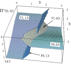
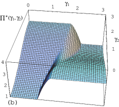
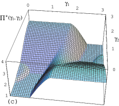
Figure 1: The quantum Nash equilibrium payoff $\Pi_{A}^{\star}(\gamma)=\Pi_{A}(\alpha^{\star},\beta^{\star};\gamma)$ (or ${\Pi}_{A}(P_{A}^{*},P_{B}^{*};\gamma)$ for mixed quantum strategies) as a function of $\gamma$. Only the region $\gamma_{1},\gamma_{2}\in[0,\pi]$ is shown since $\Pi_{A}^{\star}(\gamma)$ has the reflection invariance $\Pi_{A}^{\star}(2\pi-\gamma_{1},\gamma_{2})$ $=\Pi_{A}^{\star}(\gamma_{1},2\pi-\gamma_{2})$$=\Pi_{A}^{\star}(\gamma_{1},\gamma_{2})$. The extra invariance $\Pi_{A}^{\star}(\pi-\gamma_{1},\pi-\gamma_{2})$ $=\Pi_{A}^{\star}(\gamma_{1},\gamma_{2})$ is also visible. (a) Edge state Nash equilibria for $A_{00}\!=\!3$, $A_{01}\!=\!0$, $A_{10}\!=\!5$ and $A_{11}\!=\!1$. The value $(\gamma_{1},\gamma_{2})\!=\!(0.9272,0)$ gives the maximum payoff $\Pi_{A}^{\star}=4$ for one of the players. (b) Symmetric mixed quantum Nash equilibrium with the same parameters as (a). The maximum payoff $\Pi_{A}^{\star}=3$ is obtained at $\gamma_{2}^{\star}=0$ and $1.3694\leq\gamma_{1}^{\star}<\pi$. (c) Mixed Nash equilibrium for $A_{00}\!=\!3$, $A_{01}\!=\!0$, $A_{10}\!=\!5$ and $A_{11}\!=\!0.2$. The two bumps near the left and right ends are due the pure symmetric Nash equilibria (20).

For illustration, let us consider the case where the classical game $\gamma=0$ exhibits the Prisoner’s Dilemma, $A_{01}<$$A_{11}<$$A_{00}<$$A_{10}$. Adopting the numerical values used in EW99 , we observe from FIG. 1(a) that two asymmetric Nash equilibria coexist in the middle strip that separates the two domains where the symmetric Nash equilibria arise. The maximal payoff for player $A$ is achieved by the equilibrium strategy $\left|1,0\right>$ at the optimal choice $(\gamma_{1}^{\star},\gamma_{2}^{\star})$$=(2\arcsin\sqrt{\lambda},0)$, and also by its symmetric partner $\left|0,1\right>$ at $(\pi-2\arcsin\sqrt{\lambda},\pi)$ where we use

$$\lambda=(A_{11}-A_{01})/(A_{10}-A_{01}).$$ (17)

Interestingly, the maximal payoff is better than that obtained when the players decide to “deny” $\left|1,1\right>$ or “confess” $\left|0,0\right>$. Note that the joint strategies (1) of the players realized at these Nash equilibria are actually entangled due to the correlation factor $J(\gamma)$. Indeed, the entropy of entanglement $S(\rho_{\rm red})$ evaluated for the reduced density operator $\rho_{\rm red}$ BB96 of the optimal state reads

$$S(\rho_{\rm red})=-\lambda\log\lambda-(1-\lambda)\log(1-\lambda),$$ (18)

which is nonvanishing since $0<\lambda<1$ for the Prisoner’s Dilemma. The optimal equilibrium, however, does not provide a desired resolution for the dilemma, because it is achieved at the expense of player $B$ receiving a lower payoff. In fact, in the middle strip, the original Prisoner’s Dilemma turns into the Game of Chicken which has its own dilemma of a different kind.

Leaving the numerical example aside for now, we return to the general case, and examine the possibility of a pure Nash equilibrium which is not one of the edge states. The interference term $\Pi_{A}^{\rm in}$ now comes into play, and applying the condition for phases, $\delta_{\xi}\Pi_{A}|_{\xi=\chi=\xi^{\star}}$, we obtain

$$\cos 2\xi^{\star}=-{G_{-}(\gamma)}/{G_{+}(\gamma)}.$$ (19)

When $|G_{-}|\leq|G_{+}|$, there is an equilibrium solution $\xi=\chi=\xi^{\star}$ with the payoff $\Pi_{A}^{\rm in}=a_{0}a_{1}b_{1}b_{1}\Delta(\gamma)$, where $\Delta(\gamma)=\sqrt{G_{+}^{2}-G_{-}^{2}}$. The condition for the amplitudes $\delta_{a_{0}}\Pi_{A}=0$ and $\delta_{b_{0}}\Pi_{B}=0$ then provides, along with the edge state solutions (15), the symmetric solution,

$$a_{0}^{\star}=b_{0}^{\star}=\left({{H_{-}(\gamma)-\Delta(\gamma)}\over{H_{+}(\gamma)+H_{-}(\gamma)-2\Delta(\gamma)}}\right)^{1/2},$$ (20)

which is valid ($0\leq a_{0}^{\star}\leq 1$) if $(H_{+}-\Delta)(H_{-}-\Delta)\geq 0$. There is no asymmetric pure Nash equilibria apart from the two edge solutions.

When $|G_{-}|>|G_{+}|$, there is no dominant strategy for the phases: the player $A$ tries to top player $B$ by choosing a phase which is off by $\pi/2$ to maximize $\Pi_{A}^{\rm in}$. The player $B$ does the same, and if the game is played repeatedly, the result is a uniform random distribution for both $\xi$ and $\chi$. This is a continuous version of the paper-scissor-stone game for phases, and results in the zero average for the interference term, $\Pi_{A}^{\rm in}=0$. Thus, we reach formally the same symmetric solution (20) with $\Delta(\gamma)=0$. The existence requirement of the solution simplifies to $H_{+}H_{-}\geq 0$ for this case, and we find, from TABLE I, that the equilibrium appears precisely in the region of the asymmetric pure Nash equilibria.

The foregoing argument is made formal by considering the mixed quantum strategies specified by probability distributions $P_{A}(\alpha)$, $P_{B}(\beta)$ over the players’ actions normalized under suitable measures $d\alpha$, $d\beta$. The distribution-averaged payoff can be defined as ${\Pi}_{X}(P_{A},P_{B};\gamma)=\int d\alpha d\beta P_{A}(\alpha)\Pi_{X}(\alpha,\beta;\gamma)P_{B}(\beta)$ for $X=A,B$. The players seek a distribution $P_{A}=P_{B}=P^{\star}$ which simultaneously maximize ${\Pi}_{A}(P_{A},P_{B};\gamma)$ and ${\Pi}_{B}(P_{A},P_{B};\gamma)$. Such a distribution furnishes a mixed quantum Nash equilibrium, extending the concept of the pure quantum Nash equilibrium specified by single values of $\alpha$ and $\beta$. Note, however, that the latter is already probabilistic in terms of classical strategies, possessing a classical mixed strategy game as a subset. The former, on the other hand, is probabilistic in terms of quantum strategies, and is realized by an ensemble of quantum systems.

In FIG. 1(b), the mixed quantum Nash equilibrium payoff for the Prisoner’s Dilemma of FIG. 1(a) is shown as a function of $\gamma$. In the middle strip, asymmetric equilibria, which are known to be dynamically unstable WE95 , are now replaced by the mixed Nash equilibrium given by (20) with $\Delta(\gamma)=0$. The global maximum of the payoff $\Pi_{A}^{\star}(\gamma^{\star})=A_{00}$ is attained along the line $\gamma_{2}^{\star}=0$, $2\arcsin\sqrt{\eta}\leq\gamma_{1}^{\star}\leq\pi$ with $\eta=(A_{10}\!-\!A_{00})/(A_{10}\!-\!A_{01})$. We mention that the quantum Nash equilibrium found in EW99 corresponds to $(\gamma_{1},\gamma_{2})=$ $(\pi/2,0)$ in our scheme. Unlike the optimal point $\left|1,0\right>$, the joint strategy state of this equilibrium remains to be $\left|0,0\right>$ and hence is not entangled. In fact, the entanglement of the Nash equilibrium is inessential in this example, since the interference term vanishes for all parameter values, leaving only classically interpretable terms.

The truly quantum characteristics of the game manifests itself when the non-edge solution (20) appears. We show an example of such cases in FIG. 1(c) which is obtained by modifying the payoff parameters slightly from the previous ones. Here, the Nash equilibria (20) contributes to the increase of the payoff as seen by the convex structures at the two ends. Examination of the solution to other types of quantum games FA03 ; OZ04a would naturally be the next task.

There are several different interpretations possible for the role of the coordinator $J(\gamma)$. The first is that it furnishes the unitary family of payoff operators ${\cal A}(\gamma)$ from a given classical payoff matrix $A_{ij}$, and therefore acts independently from the two players. The second is that it acts as a collaborator to the players and serves to maximize the payoff at the Nash equilibria by tuning $\gamma$ as $\delta_{\gamma}\Pi_{A}|_{\gamma^{\star}}=0$. In the above numerical examples, we have started from the first interpretation and tacitly moved to the second. Yet another interpretation of the coordinator is that it generates quantum fluctuations for the payoffs by randomizing the parameter $\gamma$. In this case, the game is effectively given as an average over the fluctuations, and may be studied by integrating out the parameters $\gamma_{1}$ and $\gamma_{2}$. At the level of the payoff operator, the outcome is expressed as

$$\int d\gamma_{1}d\gamma_{2}\,{\cal A}(\gamma)={1\over 2}A+{1\over 2}CAC,$$ (21)

which implies that the quantum fluctuations yield quantum moderation to the game by washing out the individual’s preference.

We conclude this article by examining the quantum and classical aspects of strategies in our formulation. We first stress that our treatment is based on the full set of quantum strategies, and thus the quantum Nash equilibria obtained here are truly optimal within the entire Hilbert space.

Among the quantum Nash equilibria, those obtained within the classical family can always be simulated by some classical means, even when their joint strategy states are entangled in the Hilbert space. In a sense, these classically realizable quantum strategies are the possible link between the quantum game theory and the classical games in macroscopic social and ecological settings. In contrast, the quantum solutions that arise only with the interference terms represent the first genuinely quantum Nash equilibria, offering superior payoffs, that have no counterparts in classical strategies,

For the comprehensive classification of the quantum games in our scheme, the full analysis of the classical family is indispensable. This should also pave the way to the extension for games with more than two strategies and two players.

One of the authors (TC) thanks the members of the Institute of Particle and Nuclear Studies at KEK for the hospitality granted to him during his entended stay.

References

- (1) D.A. Meyer, Quantum strategies, Phys. Rev. Lett. 82 (1999) 1052-1055.
- (2) J. Eisert, M. Wilkens and M. Lewenstein, Quantum games and quantum strategies, Phys. Rev. Lett. 83 (1999) 3077-3080.
- (3) L. Marinatto and T. Weber, A quantum approach to static games of complete information, Phys. Lett. A272 (2000) 291-303.
- (4) R. Axelrod, The Evolution of Cooperation, (Basic Books, New York, 1984).
- (5) For a recent review, see, e.g., A. Iqbal, Studies in the theory of quantum games, arXiv.org, quant-ph/0503176.
- (6) S.C. Benjamin and P.M. Hayden, Comments on ”Quantum games and quantum strategies”, Phys. Rev. Lett. 87 (2001) 069801(1).
- (7) S.J. van Enk and R. Pike, Classical rules in quantum games, Phys. Rev. A66 (2002) 024306.
- (8) T. Cheon, Altruistic duality in evolutionary game theory, Phys. Lett. A318 (2003) 327-332.
- (9) C.H. Bennett, G. Brassard, S. Popescu, B. Schumacher, J.A. Smolin and W.K. Wootters, Purification of noisy entanglement and faithful teleportation via noisy channels, Phys. Rev. Lett. 76 (1996) 722-725.
- (10) J.W. Weibull, Evolutionary Game Theory, (MIT Press, Cambridge, 1995).
- (11) A. P. Flitney and D. Abbott, Advantage of a quantum player over a classical one in quantum games, Proc. Roy. Soc. (London) A 459 (2003) 2463-2474.
- (12) J. Shimamura, S.K. Özdemir, F. Morikoshi and N. Imoto, Quantum and classical correlations between players in game theory, J. of Phys. A37 (2004) 4423-4436.