Quantum projection filter for a highly nonlinear model in cavity QED

Abstract

Both in classical and quantum stochastic control theory a major role is played by the filtering equation, which recursively updates the information state of the system under observation. Unfortunately, the theory is plagued by infinite-dimensionality of the information state which severely limits its practical applicability, except in a few select cases (e.g. the linear Gaussian case.) One solution proposed in classical filtering theory is that of the projection filter. In this scheme, the filter is constrained to evolve in a finite-dimensional family of densities through orthogonal projection on the tangent space with respect to the Fisher metric. Here we apply this approach to the simple but highly nonlinear quantum model of optical phase bistability of a stongly coupled two-level atom in an optical cavity. We observe near-optimal performance of the quantum projection filter, demonstrating the utility of such an approach.

1 Introduction

Over the past decade it has become increasingly clear that feedback control of quantum systems is essentially a problem of stochastic control theory with partial observations [1, 2, 3]. In this context, the system and observations are generally modeled as a pair of Itô (quantum) stochastic differential equations. It is then the goal of the control engineer to find a feedback control policy, depending on the system state only through the past history of the observations, that achieves a particular control objective.

In the case of linear system dynamics and observations and Gaussian initial conditions, the so-called optimal control problem can be solved exactly both classically [4] and quantum-mechanically [1, 5] provided that a quadratic performance criterion is chosen. This means that the control objective is specified as an optimization problem, where a certain cost function (the performance criterion) of the system evolution and the control signal is to be minimized. The resulting Linear-Quadratic-Gaussian (LQG) control is widely used in many technological applications. An important feature of LQG theory is its separation structure: the optimal controller splits up into a part that updates the optimal estimate of the system state given the observations (the Kalman filter), and an optimal feedback law which is only a function of the state estimate.

It was originally suggested by Mortensen [6] that the separation structure of LQG control carries over even to the nonlinear case. The problem now separates into the nonlinear filtering problem of finding the optimal estimate of the system statistics given the observations and the optimal control problem of finding a feedback law, based only on the filtered estimate, that minimizes some performance criterion. The estimate propagated by the filter is often referred to as the information state [7] as it contains all information of the system possessed by the observer. Unfortunately, nonlinear stochastic control is plagued by two rather severe problems. First, the information state is generally infinite-dimensional even for very simple nonlinear systems [8]. Second, even in the finite-dimensional case the nonlinear optimal control problem is generally intractable. The latter can sometimes be alleviated by posing a less stringent control objective [3]. Nonetheless nonlinear stochastic control remains an extremely challenging topic, both in the classical and quantum mechanical case.

This paper is concerned with the first problem, that of infinite-dimensionality of the nonlinear information state. There is no universal solution to this problem. The most common (though rather ad hoc) approach used by engineers is known as the extended Kalman filter [9]. In this scheme, the system dynamics is linearized around the current expected system state, and a Kalman filter based on the linear approximation is used to propagate the estimate. However, aside from the fact that the method only performs well for nearly linear systems, it is not clear how it can be applied to quantum models.

A much more flexible approximation for nonlinear filtering equations was proposed by Brigo, Hanzon and LeGland [10, 11, 12], based on the differential geometric methods of information geometry [13]. In this scheme we fix a finite-dimensional family of densities that are assumed to be good approximations to the information state. Using geometric methods the filter is then constrained to evolve in this family. The finite-dimensional approximate filter obtained in this way is known as a projection filter, and often performs extremely well when the approximating family is chosen wisely. Moreover, as this approximate filter is based on the optimal nonlinear filter, instead of on the trajectories of the system state in phase space, it is readily extended to the quantum case. Though by no means a universal solution to the filtering problem, we believe that the flexibility and performance of this method likely make it widely applicable in the realistic (real-time) implementation of quantum filtering theory.

In this paper we apply the projection filtering method to a simple, but highly nonlinear quantum system: a stongly driven, strongly coupled two-level atom in a resonant single-mode optical cavity [14, 15]. The output field of such an experiment exhibits a randomly switching phase, caused by the atomic spontaneous emission. The formalism developed by Brigo et al. can be applied directly to this system if the information state (the conditional density of the atom and cavity mode) is represented as a $Q$-function [16]. Remarkably, our projection filter shows strong connections to the classical problem of filtering a random jump process in additive white noise [17, 18].

Rather than using a quasiprobability representation, a fully quantum theory of projection filtering is expressed in terms of finite-dimensional families of density operators and quantum information geometry [13]. We will present the general theory in a future publication. Nonetheless there is no theoretical objection to the approach taken in this paper. In fact, we observe numerically that the projection filter for our model has near-optimal performance, demonstrating the utility of this approach.

This paper is organized as follows. In section 2 we introduce the projection filter and the neccessary elements of information geometry. Next, in section 3, we introduce the physical model that we will be using as an example and obtain the associated filtering equation. In section 4 we obtain the projection filter for our model. Finally, in section 5, we present and discuss the results of numerical simulations.

2 Information geometry and the projection filter

2.1 The basic principle of the projection filter

Figure 1: Cartoon drawing of the projection filter. (a) The infinite-dimensional space of all densities is represented by $M$, while $S$ is a finite-dimensional submanifold. The filter, defined by a (stochastic) differential equation in $M$, flows along a (random) vector field on $M$. The flow is such that the density remains close to $S$, but $S$ is not invariant. (b) To each point $\theta\in S$ the flow associates a (random) tangent vector $X[\theta]$ which has components in both $T_{\theta}S$ and its complement. The projection filter is generated by the vector field in $TS$ that, for each $\theta$, is the orthogonal projection of $X[\theta]$ onto $T_{\theta}S$.

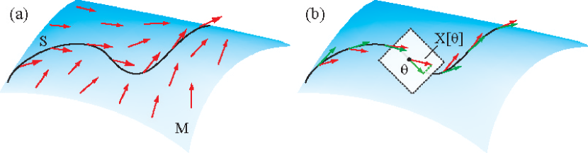
The basic idea behind the projection filter is illustrated in Figure 1. First, we assume that the information state can be represented as a probability density, i.e. an integrable nonnegative function on some underlying phase space. Though this is not always the case even in classical probability, this is generally a good assumption for any “reasonable” model. In this paper we will use a well-known quantum quasiprobability distribution, the $Q$-function [16], for this purpose. The set of all possible densities forms an infinite-dimensional function space which we will denote by $M$.

We also suppose that the information state is well approximated by densities in some finite-dimensional subspace $S$ of $M$. We will assume that $S$ can be given the structure of a differential manifold, but we do not require it to be a linear space. As such we must be careful in what follows in distinguishing between points in $S$, points in the tangent bundle $TS$, etc., as in any differential geometric situation.

In general, $S$ will not be an invariant set of the filter; if we start with a density in $S$, the filter will cause the density to evolve into a neighborhood of $S$ in $M$. The idea behind the projection filter is simply to constrain the optimal filter to remain in $S$. As $S$ is finite-dimensional, we can then express the projection filter as a differential equation in a finite set of local coordinates on $S$.

The optimal filter that propagates the information state of the system is given by a stochastic differential equation (SDE) in $M$, and we are seeking to express the projection filter as an SDE in $S$. The precise meaning of this statement is a somewhat important point which we will return to at the end of this section; for now, we can imagine the filter to be an ordinary differential equation that is driven by the observations, as follows:

$$\frac{dp_{t}}{dt}=X[p_{t};Y_{t}]$$ (1)

Here $p_{t}\in M$ is the information state and $Y_{t}$ is the observation made at time $t$. $X$, then, is an observation-dependent vector field on $M$.

To constrain the filter to evolve in $S$ we must only retain the dynamics of (1) that is parallel to $S$; dynamics perpendicular to $S$ will move the density into an undesired region. Mathematically, this idea is simply implemented if we realize that at each point $\theta\in S$, $X[\theta;Y]$ will have components both in the tangent space $T_{\theta}S$ and in its complement $T_{\theta}S^{\perp}$. We can now constrain the vector field by orthogonally projecting $X[\theta;Y]$ onto $T_{\theta}S$ for every $\theta\in S$. The resulting approximate filter, in which only the dynamics that leaves $S$ invariant is retained, is the projection filter [10, 11, 12].

Before we can flesh out the details of this scheme we must deal with the fact that the filter is not given by a differential equation as in (1), but by an SDE of the form

$$dp_{t}=A[p_{t}]\,dt+B[p_{t}]\,dY_{t}$$ (2)

We would like to think of $A+B\dot{Y}_{t}$ as a “stochastic vector field” so that we can directly apply the scheme discussed above. The theory of stochastic differential equations on manifolds [19, 20] tells us that we can in fact do this, as long as we interpret (2) as a Stratonovich SDE

$$dp_{t}=A[p_{t}]\,dt+B[p_{t}]\circ dY_{t}$$ (3)

This is not surprising as, for example, Itô’s rule is incompatible with the requirement that the Lie derivative along a vector field is a derivation [21] (in other words, a differential geometric transformation rule can only contain first derivatives, and the only stochastic integral with this property is the Stratonovich integral.) Note that usually filtering equations are given in the Itô form; hence we must transform to the Stratonovich form before we can derive the projection filter.

2.2 Information geometry

In order to perform the key step in the above procedure, the orthogonal projection, we need an inner product in the tangent space $T_{\theta}S$. A differential manifold is not naturally endowed with an inner product structure, however, and hence the projection filter is not yet well defined. We need to add to the manifold a Riemannian structure [22]. In statistics there is a natural way to do this, and the resulting theory is known as information geometry [13].

There are different ways of introducing this structure, but perhaps the easiest treatment is obtained by considering instead of the densities $M$ the space of square roots of densities $M^{1/2}$. The fact that any density is integrable guarantees that the square root of any density is square integrable; hence $M^{1/2}$ is a subspace of $L^{2}$, the space of square integrable functions, and any vector field on $M^{1/2}$ takes values in $L^{2}$.

Similarly, we consider the manifold $S^{1/2}$, which we will explicitly parametrize as

$$S^{1/2}=\{\sqrt{p(\cdot,\theta)},~~\theta\in\Theta\subset\mathbb{R}^{m}\}$$ (4)

That is, $S^{1/2}$ is a finite-dimensional manifold of square roots of densities, parametrized by the local coordinates $\theta\in\Theta$. As $S^{1/2}\subset M^{1/2}$, for any $\theta\in\Theta$ the tangent space $T_{\theta}S^{1/2}$ is the linear subspace of $L^{2}$ given by

$$T_{\theta}S^{1/2}=\mbox{Span}\left[\frac{\partial\sqrt{p(\cdot,\theta)}}{\partial\theta^{1}},\cdots,\frac{\partial\sqrt{p(\cdot,\theta)}}{\partial\theta^{m}}\right]\subset L^{2}$$ (5)

The reason for working with square roots of densities is that this gives a natural inner product in the tangent space, which is simply the standard $L^{2}$-inner product. In particular, we can calculate the associated metric tensor in the basis of (5):

$$\left\langle\frac{\partial\sqrt{p(\cdot,\theta)}}{\partial\theta^{i}},\frac{\partial\sqrt{p(\cdot,\theta)}}{\partial\theta^{j}}\right\rangle=\int\frac{\partial\sqrt{p(x,\theta)}}{\partial\theta^{i}}\frac{\partial\sqrt{p(x,\theta)}}{\partial\theta^{j}}dx=\frac{1}{4}g_{ij}(\theta)$$ (6)

Up to a factor of $1/4$, this is the well-known Fisher information matrix $g_{ij}(\theta)$.

We are now in the position to define what we mean by orthogonal projection of a vector field on $M$ onto $TS$. At each $\theta$, the orthogonal projection is

$$\Pi_{\theta}X[\theta]=\sum_{i=1}^{m}\sum_{j=1}^{m}4g^{ij}(\theta)\left\langle X[\theta],\frac{\partial\sqrt{p(\cdot,\theta)}}{\partial\theta^{j}}\right\rangle\frac{\partial\sqrt{p(\cdot,\theta)}}{\partial\theta^{i}},$$ (7)

where we have used the inverse Fisher information matrix $g^{ij}(\theta)$ to account for the fact that the basis of (5) is not orthogonal. This is the main result that is needed to obtain projection filters.

2.3 Orthogonal projection of a Stratonovich filter

Let us now discuss how to perform orthogonal projection onto a finite-dimensional manifold $S$ for the very general form (3) of a filtering equation. We begin by converting the equation to the square root form; this gives

$$d\sqrt{p_{t}}=\frac{1}{2\sqrt{p_{t}}}A[p_{t}]\,dt+\frac{1}{2\sqrt{p_{t}}}B[p_{t}]\circ dY_{t}$$ (8)

We now constrain the filter to evolve on $S^{1/2}$ through orthogonal projection:

$$d\sqrt{p(\cdot,\theta_{t})}=\Pi_{\theta_{t}}\frac{A[p(\cdot,\theta_{t})]}{2\sqrt{p(\cdot,\theta_{t})}}\,dt+\Pi_{\theta_{t}}\frac{B[p(\cdot,\theta_{t})]}{2\sqrt{p(\cdot,\theta_{t})}}\circ dY_{t}$$ (9)

This is just a finite-dimensional SDE for the parameters $\theta_{t}$. To convert the expression explicitly into this form, note that by the Stratonovich transformation rule

$$d\sqrt{p(\cdot,\theta_{t})}=\sum_{i}\frac{\partial\sqrt{p(\cdot,\theta_{t})}}{\partial\theta_{t}^{i}}\circ d\theta_{t}^{i}$$ (10)

Comparing with (7) and (9), we find that

$$d\theta_{t}^{i}=\left\langle\frac{A[p(\cdot,\theta_{t})]}{p(\cdot,\theta_{t})},\Lambda_{t}^{i}(\cdot,\theta_{t})\right\rangle dt+\left\langle\frac{B[p(\cdot,\theta_{t})]}{p(\cdot,\theta_{t})},\Lambda_{t}^{i}(\cdot,\theta_{t})\right\rangle\circ dY_{t}$$ (11)

where

$$\Lambda_{t}^{i}(\cdot,\theta_{t})=\sum_{j=1}^{m}g^{ij}(\theta_{t})\frac{\partial p(\cdot,\theta_{t})}{\partial\theta^{j}_{t}}$$ (12)

Equations (11), (12) and (6) can be used to directly calculate the projection filter for a wide range of models.

3 The physical model and the quantum filter

3.1 The Jaynes-Cummings model in the strong driving limit

Figure 2: Schematic of the experimental setup that corresponds to our model. A strongly coupled two-level atom in a resonant, single mode cavity is strongly driven by a resonant driving laser, and spontaneously emits in all directions. One of the cavity mirrors is leaky, and the atomic dynamics is observed through homodyne detection of the electromagnetic field in this forward mode.

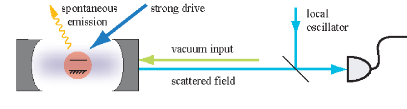
We consider the following physical system, shown in Figure 2. A two-level atom is strongly coupled to the mode of a single-mode cavity. The cavity mode and the atomic frequency are resonant. The atom is strongly driven on resonance by a laser, and spontaneously emits in all directions. A forward mode of the electromagnetic field outside the cavity, initially in the vacuum state, scatters off one of the cavity mirrors. By making this mirror slightly leaky, we extract information from the system into the external field. Homodyne detection of the forward mode then yields information about the atom and cavity.

The goal of this section is to model this physical system as a pair of Itô quantum stochastic differential equations, one of which describes the atom-cavity evolution and one describing the homodyne observations. To this end, we begin by writing down the full Hamiltonian for the system:

$$H=H_{0}+H_{d}+H_{\rm JC}+H_{f}+H_{s}$$ (13)

Here $H_{0}$ is the free Hamiltonian

$$H_{0}=\hbar\omega_{0}a^{\dagger}a+\frac{\hbar\omega_{0}}{2}\sigma_{z}+\int_{0}^{\infty}d\omega\,\hbar\omega(b_{f}^{\dagger}(\omega)b_{f}(\omega)+b_{s}^{\dagger}(\omega)b_{s}(\omega)),$$ (14)

$H_{d}$ is the drive Hamiltonian

$$H_{d}=i\hbar(\mathcal{E}/2)(e^{i\omega_{0}t}\sigma-e^{-i\omega_{0}t}\sigma^{\dagger}),$$ (15)

$H_{\rm JC}$ is the well-known Jaynes-Cummings Hamiltonian

$$H_{\rm JC}=i\hbar g(a^{\dagger}\sigma-a\sigma^{\dagger}),$$ (16)

and $H_{f}$ and $H_{s}$ are the dipole couplings to the forward and spontaneous emission field modes outside the cavity (see e.g. [23])

$$H_{f}=\hbar\int_{0}^{\infty}d\omega\,\kappa_{f}(\omega)[ab_{f}^{\dagger}(\omega)+a^{\dagger}b_{f}(\omega)]$$ (17)

$$H_{s}=\hbar\int_{0}^{\infty}d\omega\,\kappa_{s}(\omega)[\sigma b_{s}^{\dagger}(\omega)+\sigma^{\dagger}b_{s}(\omega)]$$ (18)

Here $\sigma=|g\rangle\langle e|$ is the atomic lowering operator, $\sigma_{z}=[\sigma^{\dagger},\sigma]$, $a$ is the cavity mode lowering operator (we will also use $x=a^{\dagger}+a$ and $y=i(a^{\dagger}-a)$), and $b_{f}(\omega)$ and $b_{s}(\omega)$ are the annihilators of the forward and spontaneous emission modes, respectively. The resonant frequency of the atom, drive and cavity mode is denoted by $\omega_{0}$, $\mathcal{E}$ is the drive strength, $g$ is the atom-cavity coupling strength, and $\kappa_{f}(\omega)$ and $\kappa_{s}(\omega)$ determine the frequency-dependent coupling to the external field modes.

We will assume that $\omega_{0}\gg\mathcal{E}\gg g>\kappa_{f},\kappa_{s}$. Following [15], let us switch to the interaction picture with respect to $H_{0}+H_{d}$. We obtain the interaction Hamiltonian

$$\frac{H_{\rm I}}{\hbar}=ig[a^{\dagger}\sigma(t)-a\sigma^{\dagger}(t)]+\int_{0}^{\infty}d\omega\,\kappa_{s}(\omega)[\sigma(t)b_{s}^{\dagger}(\omega)e^{i(\omega-\omega_{0})t}+\mbox{h.c.}]$$

$$\phantom{\frac{H_{\rm I}}{\hbar}=ig[a^{\dagger}\sigma(t)-a\sigma^{\dagger}(t)]}+\int_{0}^{\infty}d\omega\,\kappa_{f}(\omega)[ab_{f}^{\dagger}(\omega)e^{i(\omega-\omega_{0})t}+\mbox{h.c.}]$$ (19)

where we have defined

$$|\pm\rangle=2^{-1/2}(|g\rangle\mp i|e\rangle),~~~~\mu=|-\rangle\langle+|,~~~~\mu_{z}=[\mu^{\dagger},\mu],$$ (20)

$$\sigma(t)=(-i/2)(\mu e^{-i\mathcal{E}t}+\mu_{z}-\mu^{\dagger}e^{i\mathcal{E}t})$$ (21)

There are two time scales in the Hamiltonian (19), which we will consider separately. The first term evolves on the slow time scale of the atomic evolution. As $\mathcal{E}$ is very large compared to the atomic time scale, we make the rotating wave approximation by dropping the rapidly oscillating terms.

The remaining terms in (19) correspond to the fast time scale of interaction with the external electromagnetic field. We cannot use the rotating wave approximation for these terms, as the external fields are broadband and thus have modes that respond on the fast time scale. Instead, we make the weak coupling (Markov) approximation for these terms; this results in the following white noise Hamiltonian:

$$\tilde{H}_{\rm I}=\hbar(g/2)\mu_{z}x+\hbar\sqrt{2\kappa}\,[a\dot{B}_{f}^{\dagger}(t)+\mbox{h.c.}]+i\hbar[\sqrt{\gamma_{+}/2}\,\mu\dot{B}_{s,+}^{\dagger}(t)$$

$$\phantom{\tilde{H}_{\rm I}=\hbar(g/2)\mu_{z}x+}+\sqrt{\gamma_{z}/2}\,\mu_{z}\dot{B}_{s,z}^{\dagger}(t)+\sqrt{\gamma_{-}/2}\,\mu^{\dagger}\dot{B}_{s,-}^{\dagger}(t)-\mbox{h.c.}]$$ (22)

Here $B_{f}^{\dagger}$, $B_{s,+}^{\dagger}$, $\dot{B}_{s,z}^{\dagger}$ and $\dot{B}_{s,-}^{\dagger}$ are independent quantum white noises corresponding, respectively, to the forward channel and the three spontaneous emission channels at $\omega=\omega_{0}+\mathcal{E}$, $\omega_{0}$, and $\omega_{0}-\mathcal{E}$ (the upper, middle and lower peaks of the Mollow triplet.)

We refer to [23] for a discussion of the white noise approximation. Care must be taken to assign an independent white noise to each frequency component of $\sigma(t)$ (e.g. section III.E of [23]); each frequency probes a different subset of the modes $b(\omega)$ and hence “sees” a different noise. In the weak coupling limit these noises are in fact white and independent. For a more rigorous approach to the white noise limit see [24, 25]. Using the latter approach we can explicitly calculate $\kappa=\pi\kappa_{f}(\omega_{0})^{2}$, $\gamma_{z}=\pi\kappa_{s}(\omega_{0})^{2}$, and $\gamma_{\pm}=\pi\kappa_{s}(\omega_{0}\pm\mathcal{E})^{2}$. For simplicity, we will assume that approximately $\gamma_{z,+,-}=\gamma$.

The white noise Hamiltonian (3.1) by itself is not well defined. However, we can give rigorous meaning to the equation

$$\frac{dU_{t}}{dt}=-\frac{i}{\hbar}\tilde{H}_{\rm I}U_{t}$$ (23)

if we interpret it as a Stratonovich quantum stochastic differential equation [23, 25]. After conversion to the Itô form, this equation reads

$$dU_{t}=[\sqrt{\gamma/2}\,(\mu\,dB_{s,+}^{\dagger}(t)+\mu_{z}\,dB_{s,z}^{\dagger}(t)+\mu^{\dagger}\,dB_{s,-}^{\dagger}(t)-\mbox{h.c.})$$

$$\phantom{dU_{t}=[\sqrt{\gamma/2}}-i\sqrt{2\kappa}\,(a\,dB_{f}^{\dagger}(t)+\mbox{h.c.})$$

$$\phantom{dU_{t}=[\sqrt{\gamma/2}}-\kappa a^{\dagger}a\,dt-(\gamma/2)\,dt-i(g/2)\mu_{z}x\,dt]\,U_{t}$$ (24)

Let us now turn to the homodyne observation of the field. The homodyne detector measures a quadrature of the forward channel after it has scattered off the cavity. We will choose the quadrature $B_{f}(t)+{B_{f}}^{\dagger}(t)$; the observation process is then $Y(t)=U_{t}^{\dagger}(B_{f}(t)+{B_{f}}^{\dagger}(t))U_{t}$ (i.e., the photocurrent is $I(t)=dY(t)/dt$.) Using the quantum Itô rules [23, 26], we easily find the differential form of this expression:

$$dY(t)=\sqrt{2\kappa}\,U_{t}^{\dagger}yU_{t}\,dt+dB_{f}(t)+dB_{f}^{\dagger}(t)$$ (25)

We can slightly extend our observation model to account for technical noise, detector inefficiency, etc. To model such effects, we add to (25) an independent corrupting noise $\propto dC(t)+dC^{\dagger}(t)=dV(t)$. It is customary in the quantum optics literature to normalize $Y(t)$ so that $dY(t)^{2}=dt$. In terms of the detection efficiency $\eta\in(0,1]$

$$dY(t)=\sqrt{2\kappa\eta}\,U_{t}^{\dagger}yU_{t}\,dt+\sqrt{\eta}\,[dB_{f}(t)+dB_{f}^{\dagger}(t)]+\sqrt{1-\eta}\,dV(t)$$ (26)

We will take the Itô equations (24), (26) as our model for the system-observation pair.

3.2 The quantum filter

Now that we have a model for the system and the observation process, we can calculate the optimal filter. The derivation of the filtering equation is beyond the scope of this paper; for various approaches, see [3, 27, 28, 29, 30]. We will attempt, however, through a simple finite-dimensional analogy, to explain our interpretation of the filtering equation, as it is not entirely the same as the interpretation that is often found in the physics literature (e.g. [31]).

The optimal filter propagates the information state, which determines our best estimate of every system observable given the observations we have made. In our model, every system observable can be represented as a self-adjoint operator $X$ that lives on the atom-cavity Hilbert space; as we are working in the Heisenberg picture, this observable at time $t$ is given by $j_{t}(X)=U_{t}^{\dagger}XU_{t}$. We must now define what we mean by an estimate of an observable.

The idea behind the concept of estimation is that we have made some observation, and given the outcome of this observation we wish to make a guess as to the outcome of a different observable that we haven’t measured. That is, the estimate of an observable $X$ given an observation of $Y$ is some function $f(Y)$ whose outcome represents our best guess of $X$. To find the best estimate we must specify some cost function $\mathcal{C}[f]$ to optimize; the function that minimizes $\mathcal{C}$ is then by definition the optimal estimate.

The most commonly used estimator is one that minimizes the mean-square error

$$\mathcal{C}[f]=\langle(X-f(Y))^{2}\rangle$$ (27)

The observable $f(Y)$ that minimizes this cost is called the conditional expectation $\mathcal{E}(X|Y)$ of $X$ given $Y$. We will use the conditional expectation as our information state throughout this paper. However, note that if we had chosen a different cost we would obtain a different information state and filter. There is nothing inherently superior about the choice (27); in fact, it is sometimes advantageous to choose a different estimator with e.g. improved robustness properties [7, 32].

To understand how the conditional expectation relates to familiar notions from quantum theory, we will demonstrate the procedure using a pair of finite-dimensional observables [33]. Let $X$ and $Y$ be two $n$-dimensional observables, $n<\infty$, and let $Y$ have $m$ distinct eigenvalues $y_{i}$. Then $Y$ can be decomposed as

$$Y=\sum_{i=1}^{m}y_{i}P_{i}$$ (28)

where $P_{i}$ is the projection operator onto the eigenspace corresponding to $y_{i}$. Clearly any function of $Y$ is a linear combination of $P_{i}$, and vice versa. Hence we identify the set of all observables that are functions of $Y$ with the span of $\{P_{i}\}$. The conditional expectation $\mathcal{E}(X|Y)$ is then the element of this set that minimizes the cost (27).

To find this element, we use the following trick. The expression $\langle X^{\dagger}Y\rangle$ defines an inner product on the set of $n\times n$ complex matrices. Using this inner product, we orthogonally project $X$ onto the linear space spanned by $\{P_{i}\}$. This gives

$$P_{Y}X=\sum_{i=1}^{m}\frac{\langle P_{i}X\rangle}{\langle P_{i}\rangle}P_{i}$$ (29)

It is a well known fact that the orthogonal projection of some vector $v$ onto a linear subspace $W$ with respect to any inner product $(a,b)$ gives the element $w\in W$ that minimizes the quantity $((v-w),(v-w))$ [34]. In our case, this means that $P_{Y}X$ minimizes $\langle(X-f^{*}(Y))(X-f(Y))\rangle$. $f(Y)$ is only an observable, however, if $f$ is real, in which case we see that $P_{Y}X$ is precisely the conditional expectation $\mathcal{E}(X|Y)$. Note that the orthogonal projection $P_{Y}X$ will always be self-adjoint if $X$ and $Y$ commute.

Remarkably, when $X$ and $Y$ commute, the expression (29) is equivalent to the traditional projection postulate. To see this, note that if we observe $Y=y_{i}$ then $P_{Y}X$ takes the value $\langle P_{i}X\rangle/\langle P_{i}\rangle=\langle P_{i}XP_{i}\rangle/\langle P_{i}\rangle$, which is exactly the expectation of $X$ with respect to the initial state projected onto the eigenspace of $y_{i}$. The situation is somewhat ambiguous for noncommuting $X$ and $Y$, and we will simply refrain from defining the conditional expectation $\mathcal{E}(X|Y)$ when $[X,Y]\neq 0$.

The quantum filter determines the best estimate of every system observable given the observations; i.e., it propagates $\pi_{t}(X)=\mathcal{E}(j_{t}(X)|Y(s\leq t))$, where here $\mathcal{E}(\cdot|\cdot)$ is a proper infinite-dimensional generalization of (29). A crucial point is that $j_{t}(X)$ and $Y(s)$ can in fact be shown to commute for all $s\leq t$; this is called the nondemolition property by Belavkin [27]. Thus we see that, even though we can evidently interpret the quantum filter in terms of the projection postulate, we do not need to postulate anything beyond the standard formalism of observables and expectations in quantum mechanics. Instead, we see that the filter follows naturally from a statistical inference procedure wherein we find the least-squares estimate for every system observable given the observations. This point of view is very natural in a control-theoretic context.

We now give the quantum filter for our model (24), (26); we refer to [3, 27, 28, 29, 30] for various approaches to deriving this equation. The result is

$$d\pi_{t}(X)=\pi_{t}((\gamma/2)\{\overline{\mathcal{D}}[\mu]+\overline{\mathcal{D}}[\mu_{z}]+\overline{\mathcal{D}}[\mu^{\dagger}]\}X)\,dt$$

$$\phantom{d\pi_{t}(X)=\pi}+\pi_{t}(2\kappa\,\overline{\mathcal{D}}[a]X)\,dt+\pi_{t}(i(g/2)[\mu_{z}x,X])\,dt$$

$$\phantom{d\pi_{t}(X)=\pi}+\sqrt{2\kappa\eta}\,[i\pi_{t}(a^{\dagger}X-Xa)-\pi_{t}(y)\pi_{t}(X)]\times$$

$$\phantom{d\pi_{t}(X)=\pi+\sqrt{2\kappa\eta}\,[i\pi_{t}(a^{\dagger}X-X}(dY(t)-\sqrt{2\kappa\eta}\,\pi_{t}(y)\,dt)$$ (30)

where $\overline{\mathcal{D}}[c]X=c^{\dagger}Xc-(c^{\dagger}cX+Xc^{\dagger}c)/2$. The process $dW(t)=dY(t)-\sqrt{2\kappa\eta}\,\pi_{t}(y)\,dt$ is known as the innovations process; it describes how “surprised” we are by the measurement, as it is the difference between the observation $dY(t)$ and our best estimate of what we should observe. It can be shown that, as long as the observation process $Y(t)$ has the statistics determined by (24) and (26), the innovations process $dW_{t}$ is a Wiener process. In some sense this reflects the optimality of the filter, as it means that the innovation is unbiased.

Usually the quantum filter (30) is written in its density form. To do this, we define a random density operator $\rho_{t}$ such that $\pi_{t}(X)={\rm Tr}[X\rho_{t}]$. We then find

$$d\rho_{t}=-i(g/2)[\mu_{z}x,\rho_{t}]\,dt+2\kappa\mathcal{D}[a]\rho_{t}\,dt$$

$$\phantom{d\rho_{t}=-i}+(\gamma/2)\{\mathcal{D}[\mu]+\mathcal{D}[\mu_{z}]+\mathcal{D}[\mu^{\dagger}]\}\rho_{t}\,dt$$ (31)

$$\phantom{d\rho_{t}=-i}+\sqrt{2\kappa\eta}\,[i\rho_{t}a^{\dagger}-ia\rho_{t}-{\rm Tr}[\rho_{t}y]\rho_{t}](dY(t)-\sqrt{2\kappa\eta}\,{\rm Tr}[\rho_{t}y]\,dt)$$

where $\mathcal{D}[c]\rho=c\rho c^{\dagger}-(c^{\dagger}c\rho+\rho c^{\dagger}c)/2$. This description is more economical than the raw filter (30), and appears frequently in the physics literature. We have to be careful, however, to interpret $\rho_{t}$ as the information state of an observer with access to $Y(t)$, and not as the physical state of the system. This point will be important for the interpretation of our results.

We conclude this section with one more filter, the so-called unnormalized filter, which is given by the expression

$$d\tilde{\rho}_{t}=-i(g/2)[\mu_{z}x,\tilde{\rho}_{t}]\,dt+2\kappa\mathcal{D}[a]\tilde{\rho}_{t}\,dt$$

$$\phantom{d\rho_{t}=-i}+(\gamma/2)\{\mathcal{D}[\mu]+\mathcal{D}[\mu_{z}]+\mathcal{D}[\mu^{\dagger}]\}\tilde{\rho}_{t}\,dt$$ (32)

$$\phantom{d\rho_{t}=-i}+i\sqrt{2\kappa\eta}\,[\tilde{\rho}_{t}a^{\dagger}-a\tilde{\rho}_{t}]\,dY(t)$$

The information state $\tilde{\rho}_{t}$ propagated by this filter is not normalized, ${\rm Tr}[\tilde{\rho}_{t}]\neq 1$. However, it is simply related to the normalized information state by $\rho_{t}=\tilde{\rho}_{t}/{\rm Tr}[\tilde{\rho}_{t}]$. The chief advantage of (32) is that it is a linear equation, whereas (31) is nonlinear in $\rho_{t}$. This makes (32) somewhat easier to manipulate.

3.3 The $Q$-filter

In [15], it was noticed that density operators of the form

$$\rho=\sum_{a=\pm}|a\rangle\langle a|\otimes\int dy\,P^{a}(y)|iy/2\rangle\langle iy/2|$$ (33)

[$|iy/2\rangle$ are coherent states of the cavity mode] form an invariant set of the filtering equation (31). Thus, as long as the initial density is within this set, we can represent the filtering equations in terms of the pair of real (Glauber-Sudarshan) functions $P^{\pm}(y)$ on a line. Substituting (33) into (32) yields the unnormalized $P$-filter

$$dP^{\pm}_{t}(y)=\frac{\partial}{\partial y}[(\pm g+\kappa y)P^{\pm}_{t}(y)]\,dt$$

$$\phantom{dP^{\pm}_{t}(y)=(\pm g+}+\frac{\gamma}{2}[P^{\mp}_{t}(y)-P^{\pm}_{t}(y)]\,dt+\sqrt{2\kappa\eta}\,yP^{\pm}_{t}(y)\,dY(t)$$ (34)

For our purposes, it is more convenient to work with unnormalized $Q$-functions

$$Q^{\pm}(y)=\langle\pm,iy/2|\rho|\pm,iy/2\rangle=\int dy^{\prime}\,P^{\pm}(y^{\prime})\,e^{-(y-y^{\prime})^{2}/4}$$ (35)

as these are always guaranteed to be well-behaved densities [16]. We obtain

$$dQ^{\pm}_{t}(y)=\frac{\gamma}{2}[Q^{\mp}_{t}(y)-Q^{\pm}_{t}(y)]\,dt+\frac{\partial}{\partial y}[(\pm g+\kappa y)Q^{\pm}_{t}(y)]\,dt$$

$$\phantom{dQ^{\pm}_{t}(y)=Q}+2\kappa\frac{\partial^{2}}{\partial y^{2}}Q^{\pm}_{t}(y)\,dt+\sqrt{2\kappa\eta}\,\left[y+2\frac{\partial}{\partial y}\right]Q^{\pm}_{t}(y)\,dY(t)$$ (36)

The simplicity of this expression motivates our choice of this system for demonstrating the quantum projection filter.

Rather than using the $Q$-function for the projection filter, we could work directly with the filter (31) in density form and apply methods of quantum information geometry [13]. However, note that any metric on a manifold of densities induces a metric on the corresponding manifold of density operators (e.g. [35]). Thus even the $Q$-function projection filter is a true quantum projection filter, as long as we project onto a family of $Q$-functions that correspond to valid quantum states.

3.4 Observing the spontaneous emission

Until now we have only observed the forward channel; however, at least in principle, we could also observe independently the three spontaneous emission channels $B_{s,z}$, $B_{s,\pm}$. We would like to identify a spontaneous emission event with the detection of a photon in one of these side channels. As such, in this section we discuss the situation wherein direct photodetection is performed in each of the spontaneous emission channels, in addition to the homodyne detection of the forward channel.

The analysis in this case is very similar to the one performed in sections 3.1–3.2. The system model is still given by (24). Now, in addition to (26), we need to introduce three observation processes $N_{z,+,-}$ corresponding to photodetection (with perfect efficiency) in the three spontaneous emission channels. The details of this setup and the associated filtering equations are well known and we will not repeat them here (see e.g. [30]). The full (normalized) filtering equation is given by

$$d\rho_{t}=-i(g/2)[\mu_{z}x,\rho_{t}]\,dt+2\kappa\mathcal{D}[a]\rho_{t}\,dt$$

$$\phantom{d\rho_{t}=-i}+(\gamma/2)\{\mathcal{D}[\mu]+\mathcal{D}[\mu_{z}]+\mathcal{D}[\mu^{\dagger}]\}\rho_{t}\,dt$$

$$\phantom{d\rho_{t}=-i}+\sqrt{2\kappa\eta}\,[i\rho_{t}a^{\dagger}-ia\rho_{t}-{\rm Tr}[\rho_{t}y]\rho_{t}](dY(t)-\sqrt{2\kappa\eta}\,{\rm Tr}[\rho_{t}y]\,dt)$$

$$\phantom{d\rho_{t}=-i}+\mathcal{G}[\mu]\rho_{t}\,(dN_{+}(t)-(\gamma/2)\,{\rm Tr}[\mu^{\dagger}\mu\rho_{t}]\,dt)$$

$$\phantom{d\rho_{t}=-i}+\mathcal{G}[\mu_{z}]\rho_{t}\,(dN_{z}(t)-(\gamma/2)\,dt)$$

$$\phantom{d\rho_{t}=-i}+\mathcal{G}[\mu^{\dagger}]\rho_{t}\,(dN_{-}(t)-(\gamma/2)\,{\rm Tr}[\mu\mu^{\dagger}\rho_{t}]\,dt)$$ (37)

where $\mathcal{G}[c]\rho=c\rho c^{\dagger}/{\rm Tr}[c\rho c^{\dagger}]-\rho$. It can be shown that the statistics of the processes $N_{+,z,-}$(t) is such that they are counting processes with independent jumps and rates $(\gamma/2)\,{\rm Tr}[\mu^{\dagger}\mu\rho_{t}]$, $(\gamma/2)$ and $(\gamma/2)\,{\rm Tr}[\mu\mu^{\dagger}\rho_{t}]$, respectively.

We now have two different filters, equations (31) and (37), for the same physical system (24). To see how they relate, recall that all the filter is propagating is an information state. The information state in (31) represents the best estimate of an observer who only has access to the homodyne measurement in the forward channel. The information state in (37), however, represents the best estimate of a different observer who has access to both the homodyne observation and to direct photodetection of the spontaneous emission channels. Neither information state represents the physical state of the system; the latter is given by (24).

In practice, the frequency-resolved monitoring of spontaneously emitted photons is not (yet) experimentally feasible. Hence we would never use the filter (37) in an actual experimental situation. On the other hand, we are able to generate photocurrents $Y(t)$, $N_{+,z,-}(t)$ with the correct statistics in a computer simulation. It is then interesting to compare the estimate of an observer who has access to all photocurrents to the estimate of a realistic observer who only has access to the forward channel. In particular, this gives insight into the question asked in [15], ‘in what sense should we be able to associate observed phase-switching events [in the forward channel] with “actual” atomic decays?’

The main reason for introducing (37) is that it gives us a convenient way to perform computer simulations of the photocurrent $Y(t)$. We wish to generate sample paths of $Y(t)$, with the correct statistics, in order to compare the performance of the optimal filter (31) with the projection filter that we will derive shortly. Ideally we would directly simulate the system evolution (24); this problem is essentially intractable, however. Fortunately, we have already expressed the statistics of the photocurrents $Y(t)$, $N_{+,z,-}(t)$ completely in terms of the information state. Hence we can equivalently simulate the photocurrents by simulating (37) according to these rules ($dW(t)$ is a Wiener process, $N_{+}(t)$ has rate $(\gamma/2)\,{\rm Tr}[\mu^{\dagger}\mu\rho_{t}]$, etc.)

Of course, we can also perform such simulations with (31). However, the advantage of (37) is that, if we choose $\eta=1$, the pure states are an invariant set of this filter. We can thus rewrite the equation as a stochastic Schrödinger equation, in which we only have to propagate a vector instead of an operator. This is a much more efficient numerical procedure, and is frequently used in quantum optics [36]. For our system, the stochastic Schrödinger equation corresponding to (37) is given by

$$d|\psi_{t}\rangle=[(-i(g/2)\mu_{z}x-i\kappa\langle y\rangle_{t}a-\kappa a^{\dagger}a-(\kappa/4)\langle y\rangle_{t}^{2})\,dt$$

$$\phantom{d|\psi_{t}\rangle=[(-i}-\sqrt{2\kappa}\,(ia+\langle y\rangle_{t}/2)\,dW(t)+(\mu/\langle\mu^{\dagger}\mu\rangle_{t}^{1/2}-1)\,dN_{+}(t)$$

$$\phantom{d|\psi_{t}\rangle=[(-i}+(\mu_{z}-1)\,dN_{z}(t)+(\mu^{\dagger}/\langle\mu\mu^{\dagger}\rangle_{t}^{1/2}-1)\,dN_{-}(t)]\,|\psi_{t}\rangle$$ (38)

where $\langle c\rangle_{t}=\langle\psi_{t}|c|\psi_{t}\rangle$, and $\rho_{t}=|\psi_{t}\rangle\langle\psi_{t}|$. We numerically solve this equation in a truncated Fock basis for the cavity mode. The homodyne photocurrent (26) is calculated from the innovation using $dY(t)=\sqrt{2\kappa\eta}\,\langle y\rangle_{t}\,dt+\sqrt{\eta}\,dW_{t}+\sqrt{1-\eta}\,dV_{t}$.

4 The quantum projection filter

4.1 The finite-dimensional family

Before we can obtain a projection filter for (36), we must fix the finite-dimensional family of densities to project onto. Note that each density is actually the pair of $Q$-functions $Q^{\pm}(y)$, unlike in section 2 where each density was a single function. However, we can easily put the problem into this form by making $\pm$ an argument of the function, i.e. $Q^{\pm}(y)=Q(y,\pm)$. The square roots of $Q$-functions form a perfectly reasonable $L^{2}$ space ($L^{2}=L^{2}(\mathbb{R})\oplus L^{2}(\mathbb{R})$) with the inner product

$$\langle Q_{1}^{1/2},Q_{2}^{1/2}\rangle=\sum_{a=\pm}\int_{-\infty}^{\infty}dy\,Q_{1}^{1/2}(y,a)Q_{2}^{1/2}(y,a)$$ (39)

In the following we will use the notations $Q^{\pm}(y)$ and $Q(y,\pm)$ interchangeably.

Numerical simulations of (36) show that at any time, both $Q^{+}(y)$ and $Q^{-}(y)$ are unimodal, roughly bell-shaped densities with an approximately constant width. This suggests that we can attempt to approximate the information state by unnormalized density operators of the form

$$\rho=\nu^{+}|+\rangle\langle+|\otimes|i\mu^{+}/2\rangle\langle i\mu^{+}/2|+\nu^{-}|-\rangle\langle-|\otimes|i\mu^{-}/2\rangle\langle i\mu^{-}/2|$$ (40)

This corresponds to the bi-Gaussian family of unnormalized $Q$-functions

$$q(y,\pm)=\frac{\nu^{\pm}}{2\sqrt{\pi}}\exp\left[-\frac{(y-\mu^{\pm})^{2}}{4}\right],~\mu^{\pm}\in\mathbb{R},~\nu^{\pm}\geq 0$$ (41)

We collect the parameters into a vector $\theta=(\mu^{+},\nu^{+},\mu^{-},\nu^{-})$, where $\theta\in\Theta=\{\mu^{\pm}\in\mathbb{R},~\nu^{\pm}\geq 0\}$. Then the family of square roots of densities

$$S^{1/2}=\{\sqrt{q(y,\pm;\theta)},~\theta\in\Theta\}$$ (42)

is a finite-dimensional manifold in $L^{2}$ with the tangent space

$$T_{\theta}S^{1/2}=\mbox{Span}\left\{\frac{\partial\sqrt{q(y,\pm;\theta)}}{\partial\theta^{i}}:i=1\ldots 4\right\}$$ (43)

and Fisher metric

$$g_{ij}(\theta)=4\left\langle\frac{\partial\sqrt{q(y,\pm;\theta)}}{\partial\theta^{i}},\frac{\partial\sqrt{q(y,\pm;\theta)}}{\partial\theta^{j}}\right\rangle$$ (44)

Calculating the latter explicitly, we obtain the diagonal matrix

$$g(\theta)=\mbox{diag}\left\{\frac{\nu^{+}}{2},~\frac{1}{\nu^{+}},~\frac{\nu^{-}}{2},~\frac{1}{\nu^{-}}\right\}$$ (45)

4.2 The projection filter

We will perform projection of the unnormalized filtering equation (36), as in [18]. We begin by converting the equation into the Stratonovich form:

$$dQ^{\pm}_{t}(y)=\frac{\gamma}{2}[Q^{\mp}_{t}(y)-Q^{\pm}_{t}(y)]\,dt+\frac{\partial}{\partial y}[(\pm g+\kappa(1-4\eta)y)Q^{\pm}_{t}(y)]\,dt$$

$$\phantom{dQ^{\pm}_{t}(y)=Q}+2\kappa(1-2\eta)\frac{\partial^{2}}{\partial y^{2}}Q^{\pm}_{t}(y)\,dt+\kappa\eta(2-y^{2})Q^{\pm}_{t}(y)\,dt$$

$$\phantom{dQ^{\pm}_{t}(y)=Q+2\kappa(1-2\eta)\frac{\partial}{\partial y}}+\sqrt{2\kappa\eta}\,\left[y+2\frac{\partial}{\partial y}\right]Q^{\pm}_{t}(y)\circ dY(t)$$ (46)

We can now use (11) and (12) to find dynamical equations for the projection filter. After tedious but straightforward calculations, we obtain

$$d\nu^{+}_{t}=\left[\frac{\gamma}{2}(\nu^{-}_{t}-\nu^{+}_{t})-\kappa\eta\,(\mu^{+}_{t})^{2}\nu^{+}_{t}\right]dt+\sqrt{2\kappa\eta}\,\mu^{+}_{t}\nu^{+}_{t}\circ dY(t)$$ (47)

$$d\nu^{-}_{t}=\left[\frac{\gamma}{2}(\nu^{+}_{t}-\nu^{-}_{t})-\kappa\eta\,(\mu^{-}_{t})^{2}\nu^{-}_{t}\right]dt+\sqrt{2\kappa\eta}\,\mu^{-}_{t}\nu^{-}_{t}\circ dY(t)$$ (48)

$$\frac{d\mu^{+}_{t}}{dt}=-g-\kappa\mu^{+}_{t}+\frac{\gamma}{2}\frac{\nu^{-}_{t}}{\nu^{+}_{t}}(\mu^{-}_{t}-\mu^{+}_{t})$$ (49)

$$\frac{d\mu^{-}_{t}}{dt}=+g-\kappa\mu^{-}_{t}+\frac{\gamma}{2}\frac{\nu^{+}_{t}}{\nu^{-}_{t}}(\mu^{+}_{t}-\mu^{-}_{t})$$ (50)

Conversion to the Itô form changes (47) and (48) to

$$d\nu^{+}_{t}=\frac{\gamma}{2}(\nu^{-}_{t}-\nu^{+}_{t})\,dt+\sqrt{2\kappa\eta}\,\mu^{+}_{t}\nu^{+}_{t}\,dY(t)$$ (51)

$$d\nu^{-}_{t}=\frac{\gamma}{2}(\nu^{+}_{t}-\nu^{-}_{t})\,dt+\sqrt{2\kappa\eta}\,\mu^{-}_{t}\nu^{-}_{t}\,dY(t)$$ (52)

Finally, we rewrite the equations in terms of the normalized parameters $\mu^{\pm}$ and $\tilde{\nu}_{t}^{+}=\nu_{t}^{+}/(\nu_{t}^{+}+\nu_{t}^{-})$. This gives

$$d\tilde{\nu}^{+}_{t}=-\gamma(\tilde{\nu}^{+}_{t}-1/2)\,dt+\sqrt{2\kappa\eta}\,\tilde{\nu}^{+}_{t}(1-\tilde{\nu}^{+}_{t})(\mu^{+}_{t}-\mu^{-}_{t})\times$$

$$\phantom{d\tilde{\nu}^{+}_{t}=-\gamma(\tilde{\nu}^{+}_{t}-1/2)}\{dY(t)-\sqrt{2\kappa\eta}\,[\mu^{+}_{t}\tilde{\nu}^{+}_{t}+\mu^{-}_{t}(1-\tilde{\nu}^{+}_{t})]\,dt\}$$ (53)

$$\frac{d\mu^{+}_{t}}{dt}=-g-\kappa\mu^{+}_{t}+\frac{\gamma}{2}\frac{1-\tilde{\nu}^{+}_{t}}{\tilde{\nu}^{+}_{t}}(\mu^{-}_{t}-\mu^{+}_{t})$$ (54)

$$\frac{d\mu^{-}_{t}}{dt}=+g-\kappa\mu^{-}_{t}+\frac{\gamma}{2}\frac{\tilde{\nu}^{+}_{t}}{1-\tilde{\nu}^{+}_{t}}(\mu^{+}_{t}-\mu^{-}_{t})$$ (55)

Equations (53)–(55) form the projection filter for our model on the family $S^{1/2}$.

Note that equations (54) and (55) are singular at $\tilde{\nu}^{+}_{t}=0$ or $1$. We can trace this back to the fact that we have cheated a little in the definition of our family of densities. When $\nu^{+}=0$ (or $\nu^{-}=0$), the map $\theta\mapsto q(y,\pm;\theta)$ is not invertible, as in this case any choice of $\mu^{+}$ (or $\mu^{-}$) leads to the same density. As we have essentially inverted this map to obtain the equations (53)–(55) for the parameters, we can hardly expect these to be well-defined when this map is not invertible.

Fortunately the points $\tilde{\nu}^{+}_{t}=0$ and $1$ are never reached if we start the filter with $0<\tilde{\nu}^{+}<1$. Hence we can make the filter well-defined everywhere simply by removing the offending points $\nu^{+}_{t}=0$ and $\nu^{-}=0$ from $S^{1/2}$. The map $\theta\mapsto q(y,\pm;\theta)$ is then invertible everywhere (in other words, then the manifold is covered by a single chart.) Even if we want to consider starting the filter on $\tilde{\nu}^{+}_{t}=0$ or $1$ at $t=0$ this is not a problem; the filter dynamics will cause $\tilde{\nu}^{+}$ to evolve off the singular point, so that the filter is well defined after an arbitrarily small time step [18].

4.3 Connection with the Wonham filter

There is a remarkable connection between the projection filter obtained in the previous section and the theory of jump process filtering. This theory goes back to the beautiful classic paper by Wonham [17], in which the following problem is solved.

Denote by $x(t)$ a stationary Markovian jump process which switches between two states $a_{-}$ and $a_{+}$ with a rate $\gamma/2$; i.e., $x(t)$ is a random telegraph signal [37]. Now suppose we do not have access to a complete obeservation of $x(t)$, but only to the corrupted observation $y(t)$ defined by

$$dy(t)=\sqrt{2\kappa\eta}\,x(t)\,dt+dw(t)$$ (56)

where $dw(t)$ is a Wiener process. We can now ask, what is our best guess of the probability $p_{+}(t)$ that $x(t)=a_{+}$, given the observations $y(s\leq t)$? The answer is given in closed form by (a special case of) the Wonham filter:

$$dp_{+}(t)=-\gamma[p_{+}(t)-1/2]\,dt+\sqrt{2\kappa\eta}\,p_{+}(t)[1-p_{+}(t)](a_{+}-a_{-})\times$$

$$\phantom{dp_{+}(t)=-\gamma[p_{+}(t}\{dy(t)-\sqrt{2\kappa\eta}\,[a_{+}p_{+}(t)+a_{-}(1-p_{+}(t))]\,dt\}$$ (57)

But this is exactly (53) with $\mu^{+}_{t}$ and $\mu^{-}_{t}$ replaced by the constants $a_{+}$ and $a_{-}$.

Though intuitively appealing, this is in many ways a remarkable result. There appear to be no inherent jumps in either the optimal filter (31), or the system-observation pair (24), (26) from which it was obtained. It is true that we can choose to observe a jump process in the spontaneous emission channels, as in (37), but we could have equally chosen to perform homodyne or heterodyne detection which do not lead to jump process observations. Nonetheless (53) emerges naturally from our model, and an expression of the same form can even be obtained directly from (31) [15]. Evidently there is a deep connection between our system and the theory of jump processes.

As a classical filter, we can interpret the projection filter (53)–(55) as an adaptive Wonham filter, where the equations (54)–(55) continually adapt the parameters $a_{+}$ and $a_{-}$ in the Wonham filter (53). A similar structure was observed in [18], where the classical problem of changepoint detection (the detection of a single random jump in white noise) was treated using the projection filtering approach.

5 Numerical results

Figure 3: Comparison between the optimal and projection filters. A typical observation is shown with $\eta=1$, $g=120$, $\kappa=40$, $\gamma=20$, and the integration was performed over $25\,000$ time steps. The top row, figures (a) and (c), were calculated using the optimal filter (36); the bottom row, (b) and (d), were calculated for the same observation process using the projection filter (53)–(55).

In this section we present the results of numerical simulations of the various filters. Sample paths of the observation process were generated by numerically solving (38) with a truncated cavity basis of $25$ Fock states and the (appropriately truncated) initial state $|\psi_{0}\rangle=|-\rangle\otimes|0\rangle$. The thus generated observations were then filtered using the optimal filter in $Q$-function form (36), and using the projection filter (53)–(55).

The optimal filter was implemented using a simple finite-difference scheme [38] on a grid of $128$ equidistant points in the interval $y\in[-18,18]$, with the appropriately truncated initial condition corresponding to $|\psi_{0}\rangle$. Finally, the projection filter was started with the initial condition $\tilde{\nu}^{+}=\mu^{+}=\mu^{-}=0$, where care was taken not to propagate $\mu^{+}$ until after the first time step. In all simulations, stochastic integration was performed using the stochastic Euler method [39].

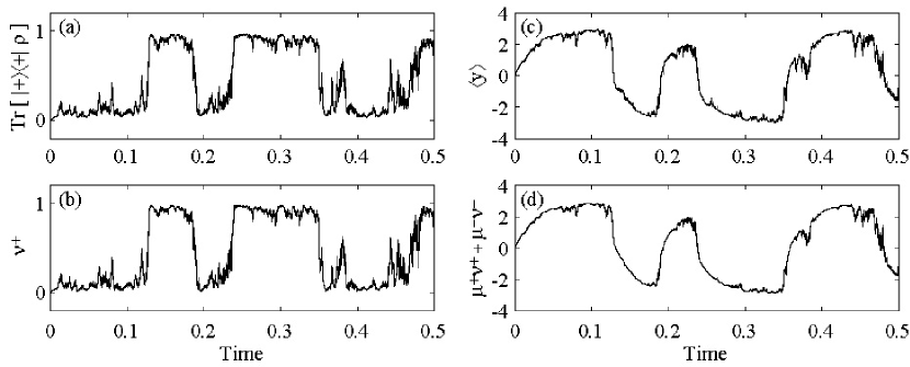
In Figure 3 a typical filtered sample path is shown. The top row was obtained from the optimal filter, while the bottom row was obtained using the projection filter. The value inferred for both the conditional probability of finding the atom in the $|+\rangle$ state (left column) and the conditional expectation of the $y$-quadrature (right column) are nearly identical for the two filters. Evidently the projection filter is an extremely good approximation to the optimal filtering equation.

Figure 4: A single run of an experiment is simulated. The dashed line (red) corresponds to the optimal estimate of an observer who has access to direct photodetection of the spontaneously emitted photons, as well as homodyne detection of the forward channel. The solid line (green) is the optimal estimate of a different observer, who only has access to the homodyne photocurrent, for the same run of the experiment. The dotted line (blue) is the projection filter estimate based only on the homodyne photocurrent. All parameters are the same as in Figure 3.

Figure 5: Two more sample paths of the filtered estimate of atomic state, demonstrating missed jumps (top) and false jumps (bottom). All parameters are the same as in Figure 3.

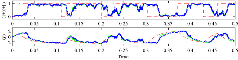
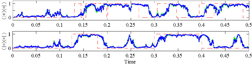
Next, in Figure 4, we compare the information state of the optimal and projection filters to the information state that is based on the additional observation of spontaneously emitted photons. The latter filter demonstrates the behavior reported in [14]. Whenever a photon is observed in one of the side peaks of the Mollow triplet, the observer infers that the atom has made a jump. The estimated phase of the cavity field then exponentially decays to a steady-state level of $\langle y\rangle=\pm g/\kappa$.

If we do not measure the spontaneous emission, our best guess of the atomic state still behaves in a jump-like way. However, we see that there is a little delay between the time that the observer of spontaneous emission thinks the atom has jumped, and the time that the homodyne observer comes to the same conclusion. If we identify atomic decay with the spontaneous emission of a photon, we can now give a fairly satisfactory answer to the question posed in [15]: ‘In what sense should we be able to associate observed phase switching events with “actual” atomic decays’? It appears that an observed phase switch signals that, had we been making such an observation, we would likely have seen a spontaneously emitted photon a little while earlier.

The detection delay is a rather generic property of the type of filtering problems we are considering [18, 40]. Any time we see a large fluctuation in the observed process, the filter has to decide whether this is a large fluctuation of the noise, or a large fluctuation of the observed system. As is pointed out by Shiryaev [40] in the context of changepoint detection, the filter rides a delicate balance between minimizing the delay time and minimizing the probability of “false alarms”. Decreasing the number of false alarms (by choosing a different filtering cost) would unavoidably increase the delay time, and vice versa. In our system, false alarms are missed jumps and false jumps; these do occur, as can be seen in Figure 5.

Figure 6: A typical filtered sample path with $\eta=1$, $g=600$, $\kappa=200$, $\gamma=20$. The integration was performed over $100\,000$ time steps. The various line types are as in the previous figures.

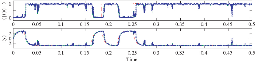
If we wish to generally improve the quality of detection we have no alternative than to increase the signal-to-noise level of the observation. In the case of our system, we can do this if we increase $g$ and $\kappa$ while keeping their ratio fixed (the analogy can be justified from (56); the signal $x$ has fixed magnitude $x=\pm g/\kappa$, while the signal-to-noise ratio $\sim g/\sqrt{\kappa}$.) A simulation with greatly increased signal-to-noise is shown in Figure 6. In this very strong coupling and damping regime, it appears that not much more information can be extracted from observation of the spontaneous emission than we could have already inferred from the homodyne photocurrent.

6 Conclusion

In this paper, we have suggested that the method of projection filtering can be very fruitful when applied to quantum filtering theory. Using a simple model of a strongly coupled two-level atom in a cavity we numerically demonstrated near-optimal performance of the projection filter, as is evident from Figures 3–6. We have also shown a connection between this model from cavity QED and the classical Wonham filter; the projection filter can be interpreted as an adaptive Wonham filter, applied to a quantum model. In future work we will develop a “true” quantum formalism for projection filtering, using methods from quantum information geometry.

The reduction of infinite or high-dimensional filters to a tractable set of equations is essential if we wish to perform estimation in real time, for example in a feedback control loop. In a control-theoretic context, converting a large, complex system into a set of simple equations is known as model reduction. Ideally, however, such a procedure should yield some bounds on the error of approximation; in our case we have observed numerically that the approximation error is very small, but we have no rigorous bounds to back up this statement. In classical control theory of linear systems, the method of balanced truncation [41] gives a very general method for model reduction with guaranteed error bounds. How to do this effectively for nonlinear systems is still an open problem, however, both in classical and in quantum theory.

References

- [1] V. P. Belavkin. Nondemolition measurements, nonlinear filtering and dynamic programming of quantum stochastic processes. In Proceedings, Bellman Continuum, Sophia-Antipolis 1988, Lecture Notes in Control and Information Sciences 121, pages 245–265. Springer-Verlag, 1988.
- [2] A. C. Doherty, S. Habib, K. Jacobs, H. Mabuchi, and S. M. Tan. Quantum feedback control and classical control theory. Phys. Rev. A, 62:012105, 2000.
- [3] R. Van Handel, J. K. Stockton, and H. Mabuchi. Feedback control of quantum state reduction, 2005. To appear in IEEE Trans. Automat. Control.
- [4] A. Bensoussan. Stochastic Control of Partially Observable Systems. Cambridge University Press, 1992.
- [5] A. C. Doherty and K. Jacobs. Feedback control of quantum systems using continuous state estimation. Phys. Rev. A, 60:2700–2711, 1999.
- [6] R. E. Mortensen. Stochastic optimal control with noisy observations. Int. J. Control, 4:455–464, 1966.
- [7] M. R. James. A quantum Langevin formulation of risk-sensitive optimal control. quant-ph/0412091, 2004.
- [8] M. Hazewinkel, S. I. Marcus, and H. J. Sussmann. Nonexistence of finite-dimensional filters for conditional statistics of the cubic sensor problem. Syst. Contr. Lett., 3:331–340, 1983.
- [9] O. L. R. Jacobs. Introduction to Control Theory. Oxford University Press, second edition, 1993.
- [10] D. Brigo, B. Hanzon, and F. LeGland. A differential geometric approach to nonlinear filtering: the projection filter. IEEE Trans. Automat. Control, 43:247–252, 1998.
- [11] D. Brigo, B. Hanzon, and F. LeGland. Approximate filtering by projection on the manifold of exponential densities. Bernoulli, 5:495–543, 1999.
- [12] D. Brigo. Filtering by projection on the manifold of exponential densities, 1996. Ph.D. thesis, Department of Economics and Econometrics, Vrije Universiteit, Amsterdam.
- [13] S. Amari and H. Nagaoka. Methods of Information Geometry. Oxford University Press, 2000.
- [14] P. Alsing and H. J. Carmichael. Spontaneous dressed-state polarization of a coupled atom and cavity mode. Quantum Opt., 3:13–32, 1991.
- [15] H. Mabuchi and H. M. Wiseman. Retroactive quantum jumps in a strongly coupled atom-field system. Phys. Rev. Lett., 81:4620–4623, 1998.
- [16] L. Mandel and E. Wolf. Optical Coherence and Quantum Optics. Cambridge University Press, 1995.
- [17] W. Wonham. Some applications of stochastic differential equations to optimal nonlinear filtering. SIAM J. Control, 2:347–369, 1965.
- [18] M. H. Vellekoop and J. M. C. Clark. A nonlinear filtering approach to changepoint detection problems: Direct and differential-geometric methods. SIAM J. Control Optim., 42:469–494, 2003.
- [19] J.-M. Bismut. Mécanique Aléatoire. Lecture Notes in Mathematics 866. Springer-Verlag, 1981.
- [20] L. C. G. Rogers and D. Williams. Diffusions, Markov Processes and Martingales, Volume 2: Itô calculus. Cambridge University Press, second edition, 2000.
- [21] R. Abraham, J. E. Marsden, and T. Ratiu. Manifolds, Tensor Analysis, and Applications. Springer, 1988.
- [22] S. Gallot, D. Hulin, and J. Lafontaine. Riemannian geometry. Springer, 2004.
- [23] C. W. Gardiner and M. J. Collett. Input and output in damped quantum systems: Quantum stochastic differential equations and the master equation. Phys. Rev. A, 31:3761–3774, 1985.
- [24] L. Accardi, Y. G. Lu, and I. Volovich. Quantum Theory and its Stochastic Limit. Springer-Verlag, 2002.
- [25] J. Gough. Quantum flows as Markovian limit of emission, absorption and scattering interactions. Commun. Math. Phys., 254:489–512, 2005.
- [26] R. L. Hudson and K. R. Parthasarathy. Quantum Itô’s formula and stochastic evolutions. Commun. Math. Phys., 93:301–323, 1984.
- [27] V. P. Belavkin. Quantum stochastic calculus and quantum nonlinear filtering. J. Multivariate Anal., 42:171–201, 1992.
- [28] V. P. Belavkin. Quantum diffusion, measurement and filtering I. Theory Probab. Appl., 38:573–585, 1994.
- [29] V. P. Belavkin. Quantum continual measurements and a posteriori collapse on CCR. Commun. Math. Phys., 146:611–635, 1992.
- [30] L. Bouten, M. Guţă, and H. Maassen. Stochastic Schrödinger equations. J. Phys. A, 37:3189–3209, 2004.
- [31] H. M. Wiseman. Quantum trajectories and quantum measurement theory. Quantum Semiclass. Opt., 8:205–222, 1996.
- [32] R. K. Boel, M. R. James, and I. R. Petersen. Robustness and risk-sensitive filtering. IEEE Trans. Automat. Control, 47:451–461, 2002.
- [33] H. Maassen. Quantum probability applied to the damped harmonic oscillator. In S. Attal and J. M. Lindsay, editors, Quantum Probability Communications XII, pages 23–58. World Scientific, 2003.
- [34] A. W. Naylor and G. R. Sell. Linear Operator Theory in Engineering and Science. Springer, 1982.
- [35] K. Życzkowski and W. Słomczyński. The Monge distance between quantum states. J. Phys. A, 31:9095–9104, 1998.
- [36] C. W. Gardiner, A. S. Parkins, and P. Zoller. Wave-function quantum stochastic differential equations and quantum-jump simulation methods. Phys. Rev. A, 46:4363–4381, 1992.
- [37] C. W. Gardiner. Handbook of Stochastic Methods for Physics, Chemistry and the Natural Sciences. Springer, 2nd edition, 1985.
- [38] W. H. Press, B. P. Flannery, S. A. Teukolsky, and W. T. Vetterling. Numerical Recipes in C: The Art of Scientific Computing. Cambridge University Press, 2nd edition, 1992.
- [39] P. E. Kloeden, E. Platen, and H. Schurz. Numerical Solution of SDE Through Computer Experiments. Springer-Verlag, 1997.
- [40] A. N. Shiryaev. On optimum methods in quickest detection problems. Theory Probab. Appl., 8:22–46, 1963.
- [41] G. E. Dullerud and F. Paganini. A course in robust control theory: a convex approach. Springer, 2000.