Violation of the entropic area law for Fermions
Abstract
We investigate the scaling of the entanglement entropy in an infinite translational invariant Fermionic system of any spatial dimension. The states under consideration are ground states and excitations of tight-binding Hamiltonians with arbitrary interactions. We show that the entropy of a finite region typically scales with the area of the surface times a logarithmic correction. Thus, in contrast to analogous Bosonic systems, the entropic area law is violated for Fermions. The relation between the entanglement entropy and the structure of the Fermi surface is discussed, and it is proven, that the presented scaling law holds whenever the Fermi surface is finite. This is in particular true for all ground states of Hamiltonians with finite range interactions.
Entanglement is a phenomenon of common interest in the fields of quantum information and condensed matter theory. It is an essential resource for quantum information processing and intimately connected with exciting quantum phenomena like superconductivity, the fractional quantum Hall effect or quantum phase transitions. Crucial to all these effects are quantum correlations, i.e., the entanglement properties, of ground states. These have recently attracted a lot of attention, leading to new insight into quantum phase transitions and renormalization group transformations rgflows and triggering the development of new powerful numerical algorithms numerics .
A fundamental question in this field is concerned with the scaling of the entropy—which is for pure states synonymous with the entanglement. That is, given a ground state of a translational invariant system, how does the entropy of a subsystem grow with the size of the considered region? Originally, this question appeared first in the context of black holes, where it is known that the Bekenstein entropy beckenstein is proportional to the area of the horizon, which led to the famous conjecture now known as the holographic principle holo ; holo2 . The renewed interest, however, comes more from the investigation of spin systems and quantum phase transitions. Moreover, the scaling of the entropy is of particular interest concerning the choice of the right ansatz-states in simulation algorithms.
In the last years, especially one-dimensional spin chains have been studied extensively and it is now believed that the entropy diverges logarithmically with the size of a block if the system is critical, and that it saturates at a finite value otherwise Latorre . For a number of models Peschel ; Korepin1 ; random2 , in particular those related to conformal field theories in 1+1 dimensions Korepin2 ; CFT , this could be shown analytically revealing a remarkable connection between the entropy growth and the universality class of the underlying theory. At the same time the diverging number of relevant degrees of freedom provides a simple understanding of the failure of DMRG methods for critical spin-chains.
For several spatial dimensions a suggested entropic area law harm1 could recently be proven harm2 for the case of a lattice of quantum harmonic oscillators (quasi-free Bosons), where again the entropy grows asymptotically proportional to the surface. On heuristic grounds this can be understood from the fact the system is non-critical: an energy gap gives rise to a finite correlation length, which in turn defines the scale on which modes inside the subsystem are correlated with the exterior. Although a general area law for gapped lattice systems has not been proven so far, the case of quasi-free Bosons is often considered as paradigmatic. In fact, recently developed simulation algorithms based on ansatz-states exhibiting the presumed entropy scaling are highly promising numerics .
The fact that in some 1- systems a vanishing energy gap leading to a diverging correlation length results in the logarithmically diverging entanglement entropy inevitably raises the question about the behavior of gapless systems in more than one dimension.
The present paper is devoted to the study of the entanglement entropy in gapless Fermionic systems of arbitrary spatial dimensions. We establish a relation between the structure of the Fermi sea and the scaling of the entropy and prove that a finite non-zero Fermi surface implies that the entanglement grows proportional to the surface of the subsystem times a logarithmic correction, i.e.,
| (1) |
if the system under consideration is a -dimensional cube with edge length . Thus, in contrast to analogous Bosonic systems the entropic area law is violated for Fermions.
Before we start to prove this result a brief discussion of the notion of locality—necessary for the concept of entanglement—is in order. In spin systems as well as in the Bosonic case of harmonic oscillators the tensor product structure of the underlying Hilbert space naturally leads to an unambiguous notion of locality. In the absence of such a tensor product structure either in general quantum field theory settings VW or in the present case of Fermions BK , one has to identify commuting subalgebras of observables and assign them to different parties. In our case the relevant algebra is the one spanned by the Fermionic creation and annihilation operators and satisfying the usual anti-commutation relations. We assign the modes with to one party (the interior) and the other modes to the other party (the exterior). Then parity conservation or even stronger, particle conservation Wick , leads to a superselection rule, which implies that all physical operators acting on commute with those acting on , leading to well-defined notions of locality and entanglement.
Let us now introduce the prerequisits for the proof. Consider a number preserving quadratic Hamiltonian
| (2) |
describing Fermions on a -dimensional cubic lattice, so that each component of the vector indices corresponds to one spatial dimension. Translation symmetry is reflected by the fact that is a Toeplitz operator, i.e., depends only on the distance between two lattice points. The Hamiltonian (2) is diagonalized by a Fourier transform leading to the dispersion relation
| (3) |
All thermal and excited states of the Hamiltonian are Fermionic Gaussian state SB04 , which are completely characterized by their correlation matrix
| (4) |
The correlation matrix describes a pure state iff , so that all eigenvalues of are , and the ground state correlation matrix is given by . Ground states for different Fermion densities are then obtained by adding a chemical potential, i.e., replacing by . If we characterize the Fermi sea by the corresponding indicator function , then the respective correlation matrix is given by Fermitheta
| (5) |
Note that this characterizes not only ground states but pure Gaussian states in their most general form (as long as they obey particle conservation and translation symmetry).
The state of a subsystem, e.g., a cube with edge length , is described by the corresponding sub-matrix of , which we will denote by . This subsystem can be decomposed into normal modes by a canonical transformation from such that the state of each normal mode has a Fock space representation of the form
| (6) |
where the are the eigenvalues of . The entropy of the subsystem can then be expressed as
| (7) | |||||
| (8) |
Since a direct computation of via the diagonalization of is yet highly non-trivial in the simplest one-dimensional case with nearest neighbor interaction Korepin1 , one relies in general on finding good bounds on the entropy. We will use quadratic bounds on of the form Fannes . The best lower bound is given by leading to
| (9) |
The set of tight quadratic upper bounds can be parameterized by the point for which become tangent x0 . We will couple this bound to the block size via , where . Straight forward but lengthy calculations show then that the entropy as a function of is asymptotically upper bounded Landau by
| (10) |
Hence, together with the lower bound this means that essentially determines the asymptotic scaling of the entropy.
The necessity of coupling the upper bound to can easily be understood physically, when one recalls that there is always a choice of the local basis in which each normal mode inside the block is only correlated with at most one mode outside BR04 . With increasing block size, more and more modes inside lose their correlations with the exterior, such that the number of nearly pure normal modes dominates more and more. Since the corresponding eigenvalues are , the point , for which the bound is tight, should tend to 1 as . Setting right from the beginning is, however, not possible since the derivative of at this point diverges.
Let us now investigate the scaling of . To this end we introduce the positive Fejér kernel DM
| (11) |
and we will abbreviate by . Then following Eq.(5) we have
| (12) | |||||
| (13) |
To further evaluate Eq.(12) we have to exploit the fact that with increasing the Fejér kernel becomes more and more concentrated around . In fact, , and for all there exists a finite constant such that
| (14) |
The crucial point here is that does not depend on . Hence, the asymptotic scaling of the entropy depends only on the behavior of the function in an -neighborhood of the origin.
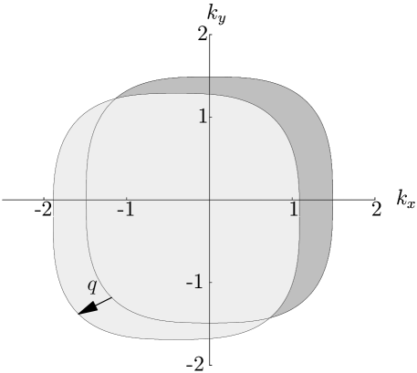
The function has a very intuitive interpretation: it is the volume of the part of the Fermi sea in -space, which is no longer covered if we shift the Fermi surface by a vector (see Fig.1). So what is the behavior of near the origin? Obviously, and . Moreover, will typically not be differentiable at , but it will rather have the structure of a pointed cone.
Let us assume that the Fermi sea is a set of non-zero measure with a finite non-zero surface. This means in particular, that almost all points with are interior points of the Fermi sea and it implies that is a continuous function in -space continuity . In fact, an infinite boundary could lead to a discontinuity of at the origin. This restriction excludes both, trivial cases (zero entropy due to zero surface) and exotic cases (fractal or Cantor set like Fermi seas). For all other cases it enables us to bound in a neighborhood of the origin by pointed cones in the following manner: consider the surface of the closed interior of the Fermi sea in one unit cell of the reciprocal lattice. Let be the area of the projection of this surface onto the hyper-plane with normal vector , where we account for each front of the surface. If, for example, the Fermi sea consist out of two disjoint three-dimensional spheres with radius , then in every direction. Since is the volume in which the Fermi sea changes upon shifting it by , we have in an -neighborhood of the origin that is given by . Using the fact that the Fermi surface is assumed to be finite we know that is bounded from above by a finite constant . Let us assume for the moment that there exists a non-zero lower bound as well. Then we can bound the integral in Eq.(14) by replacing with . Exploiting further that and that is symmetric, leads to upper and lower bounds which are up to a finite constant given by
The remaining integral is the Fejér sum of a linear function, which can be evaluated Landau to
| (16) | |||||
where is Euler’s constant and denotes the digamma function.
We still have to discuss the case . In this case we have to use different linear bounds for different directions in Eq.(Violation of the entropic area law for Fermions). Since will be larger than some at least in one direction, we are in the end led to the same type of integral and thus to the same asymptotic scaling.
Putting it all together we have indeed that scales as since all the involved constants are finite and depend not on but merely on the structure of the Fermi sea. The above argumentation holds under the assumption that the Fermi surface is not too exotic. However, if the interactions are finite in range, then the Fermi surface of the ground state is differentiable to infinite order and it is in particular finite. In general, however, one has to check whether or not the structure of the Fermi sea gives rise to an infinite slope or a discontinuity of at the origin.
The existence of Fermi surfaces leading to a scaling of the entanglement entropy which surpasses the above law, can easily be understood: consider a Fermi sea given by a checkerboard with squares of edge length . Then shifting the Fermi surface by along any lattice axis yields such that a naive limit would indeed give rise to a scaling of the entropy. Needless to say that the checkerboard does not have a well-defined limit—however, following the same idea, more sophisticated Cantor set like constructions will do the same job without any caveat. In fact, for such states were constructed in Fannes .
Remarkably, fractal or Cantor set like structures are known to appear in tight binding models. The most prominent example is the Azbel-Hofstadter Hamiltonian AB with non-integer flux, leading to the famous Hofstadter butterfly for the spectrum. Since the interaction matrix (with being the vector potential) is quasi-periodic and not translational invariant, this case is, however, not directly covered by the above argumentation. The question, which physically interesting translational invariant Hamiltonians give rise to a violation of the above scaling law via a fractional Fermi sea, remains an interesting problem for future research.
In conclusion we derived a method of relating the structure of the Fermi sea in tight-binding models to the scaling of the entanglement entropy. For every finite non-zero Fermi surface we proved the violation of a strict area law (as it is assumed for non-critical systems harm1 ; harm2 ; Zanardi ) by a logarithmic correction, i.e.,
| (17) |
with constants depending only on the Fermi sea. By the strong sub-additivity of the entropy the same scaling behavior holds true also for other regions, e.g. spheres, as long as they can be nested into two cubes of edge lengths and with independent of . The additional in the upper bound is presumably an artefact (cf. random2 ; other ) coming from the incompatibility of tight quadratic upper bounds with the binary entropy function at .
Note finally, that the derived result can be applied to spin models in one dimension random2 ; Fannes . In this case a Jordan-Wigner transformation maps Fermionic operators onto Pauli spin operators such that every tight-binding Hamiltonian with nearest neighbor interactions in Eq.(2) is then mapped onto a spin Hamiltonian of the form
| (19) | |||||
with some couplings . Conversely, every such Hamiltonian is
covered by Eq.(2), and we are in general allowed to add
arbitrary interaction terms differing from those in
Eqs.(19,19) by a sequence of s in between
every two Pauli operators. For higher dimensions, however, an
analogous construction fails, since then Jordan-Wigner
transformations do no longer preserve locality.
Acknowledgements The author thanks T. Cubitt, J. Eisert, D.
Porras and I. Cirac for valuable discussions and D. Gioev and I.
Klich, who addressed the same question independently other ,
for bringing Ref. Fannes to his attention.
References
- (1) F. Verstraete, J.I. Cirac, J.I. Latorre, E. Rico, M.M. Wolf, Phys. Rev. Lett. 94, 140601 (2005); J.I. Latorre, C.A. Lütken, E. Rico, G. Vidal, Phys. Rev. A 71, 034301 (2005).
- (2) F. Verstraete, D. Porras, J.I. Cirac, Phys. Rev. Lett. 93, 227205 (2004); F. Verstraete, J.I. Cirac, cond-mat/0407066 (2004); V. Murg, F. Verstraete, J.I. Cirac, Phys. Rev. Lett. 95, 057206 (2005); M. Zwolak, G. Vidal, Phys. Rev. Lett. 93, 207205 (2004); G. Vidal, Phys. Rev. Lett. 93, 040502 (2004).
- (3) J.D. Bekenstein, Phys. Rev. D 7, 2333 (1973).
- (4) R. Bousso, Rev. Mod. Phys. 74, 825 (2002).
- (5) Despite the motivation for harm1 the relation to black hole entropies and the holographic principle is not entirely clear holo . After all, gravity does not enter and the size of the Hilbert space is a priori unrelated to the entanglement entropy.
- (6) G. Vidal, J.I. Latorre, E. Rico, A. Kitaev, Phys. Rev. Lett. 90, 227902 (2003); J. I. Latorre, E. Rico, G. Vidal, Quant. Inf. Comp. 4 (1), 48 (2004).
- (7) I. Peschel, J. Stat. Mech. P12005 (2004); I. Peschel, cond-mat/0502034 (2005).
- (8) A.R. Its, B.-Q. Jin, V.E. Korepin, Journal Phys. A 38, 2975 (2005); B.-Q. Jin, V.E. Korepin, J. Stat. Phys. 116, 79 (2004); G. Refael, J.E. Moore Phys. Rev. Lett. 93, 260602 (2004).
- (9) J.P. Keating, F. Mezzadri, Phys. Rev. Lett. 94, 050501 (2005).
- (10) V. Korepin, Phys. Rev. Lett. 92, 096402 (2004);
- (11) P. Calabrese, J. Cardy, J. Stat. Mech. P06002 (2004).
- (12) L.Bombelli, R.K. Koul, J. Lee, R.D. Sorkin, Phys. Rev. D 34, 373 (1986); M. Srednicki, Phys. Rev. Lett. 71, 666 (1993).
- (13) M.B. Plenio, J. Eisert, J. Dreissig, M. Cramer, Phys. Rev. Lett. 94, 060503 (2005).
- (14) D. Gioev, I. Klich, quant-ph/0504151 (2005).
- (15) R. Verch, R.F. Werner, quant-ph/0403089 (2004).
- (16) S.B. Bravyi, A.Yu. Kitaev, Ann. Phys. 298, 210 (2002).
- (17) G.C. Wick, A.S. Wightman, E.P. Wigner, Phys. Rev. 88, 101 (1952); G.C. Wick, A.S. Wightman, E.P. Wigner, Phys. Rev. D 1, 3267 (1970).
- (18) H. Dym, H.P. McKean, Fourier series and integrals, Academic Press (1972).
- (19) S. Bravyi, Quantum Inf. Comp., 5(3), 216 (2005).
- (20) is a function in -space which is one if the wave vector is inside the Fermi sea, and zero otherwise. For ground states .
- (21) M. Fannes, B. Haegeman, M. Mosonyi, math-ph/0306055 (2003).
-
(22)
The upper bound , which is tight at , is found by solving and . This gives
- (23) Here Landau’s asymptotic notation is used: means that for some constant .
- (24) A.Botero, B. Reznik, Physics Letters A 331, 39 (2004).
- (25) In fact, , where is the area of the Fermi surface.
- (26) M.Ya. Azbel, Sov. Phys. JETP 19, 634 (1964); D.R. Hofstadter, Phys. Rev. B 14, 2239 (1976); P.B. Wiegmann, A.V. Zabrodin, Phys. Rev. Lett. 72, 1890 (1994).
- (27) A. Hamma, R. Ionicioiu, P. Zanardi Phys. Rev. A 71, 022315 (2005); A. Hamma, R. Ionicioiu, P. Zanardi, Phys. Lett. A 337, 22 (2005).
