Simulation of a Heisenberg XY- chain and realization of a perfect state transfer algorithm using liquid nuclear magnetic resonance

Abstract

The three- spin chain with Heisenberg XY- interaction is simulated in a three- qubit nuclear magnetic resonance (NMR) quantum computer. The evolution caused by the XY- interaction is decomposed into a series of single- spin rotations and the $J$- coupling evolutions between the neighboring spins. The perfect state transfer (PST) algorithm proposed by M. Christandl et al [Phys. Rev. Lett, 92, 187902(2004)] is realized in the XY- chain.

I Introduction

In 1982, R. P. Feynman proposed the idea of quantum computer, and pointed out that a quantum computer can simulate physics more efficiently than its classical counterpart Feynman82 . The information carriers for quantum computation are qubits. Unlike a classical bit, a qubit can lie in a superposition of two states, according to the quantum mechanical principle of superposition. Essentially, the superpositions of quantum states lead to the advantages of the quantum computers over the classical computers. The quantum gates and quantum networks proposed by D. Deutsch provide a convenient method for people to think about how to build a quantum computer in a similar way to build a classical computer Deutsch85 ; Deutsch89 . His work can be thought as a milestone in the history of quantum computerSteane98 . The current quantum network theory has shown that it is possible to construct an arbitrary $n$-qubit quantum gate by using only a finite set of single- qubit gates and two- qubit gates 4 ; 5 , so that these basic quantum gates are universal for quantum computation 6 ; 7 ; 8 . The prime factorization algorithm proposed by P. W. Shor Shor94 and the quantum search algorithm proposed by L. K. Grover Grover97 show the potential advantages of the quantum computers and accelerate the development of quantum computation.

There are several physical systems that can implement quantum computation. They are liquid nuclear magnetic resonance (NMR) Vandersypen04 , quantum dots Loss98 ; Loss99 , solid NMR Kane ; Ladd ; Suter , electron spins Vrijen , trapped ions Zoller95 ; Zoller00 , superconduction qubits Makhlin ; Devoret , and cavity QED systems Sleator ; Gigovannetti ; Yamaguchi ; Zheng . Because of its technologic maturation and convenience in manipulation, liquid NMR has been an important experimental method to implement quantum algorithm, error-correcting code, and simulate quantum systems 2 ; Boulant ; Miquel ; Lloyd ; Boghosian ; Somaroo ; Du1 ; Du2 ; zhangpra ; zhangjopb ; Peng ; Negrevergne ; Yang .

In the above systems, the interactions between qubits, at least between the neighboring qubits, are necessary for quantum computation. The Heisenberg interaction naturally exists in the various spin systems. In the liquid NMR system, the Heisenberg interaction exists in form of Ising interaction Gunlycke . In the other systems, the Heisenberg interaction takes more various forms. D. P. DiVincenzo et al pointed out that the Heisenberg interaction alone can be universal for quantum computation, if the coded qubit states are introduce DiVincenzo ; Bacon ; Knill . This result is exciting, because the single- spin operations, which usually cause additional difficulties in manipulations in some systems, can be avoided. The perfect state transfer (PST) algorithm proposed by M. Christandl et al satisfies such a condition that no single-spin operations are needed Christandl . The algorithm can transfer an arbitrary quantum state between the two ends of a spin chain or a more complex spin network in a fixed period time only using the XY- interaction. If the state is transferred in a more than three spin chain, the coded qubits are needed, so that the chain is extended to a network. Compared with the state transfer based on SWAP operations, where single-spin operations are used to switch on or off the couplings between spins Madi , the PST algorithm is easy to implement in some solid systems.

The Heisenberg interaction is expected to play an important role in building large- scale quantum computers, and it has become an interesting topic in the field of quantum information. M. C. Arnesen et al’ work indicated that the quantum entanglement phase transition occurs in the one dimension Heisenberg model Arnesen . L. Zhou et al pointed out that the thermal entanglement can be enhanced in an anisotropic Heisenberg XYZ chainZhou . J. P. Keating et al separated a quantum spin chain into two parts, and computed the entropy of entanglement between them Keating . M. Mohseni et al proposed a fault-tolerant quantum computation using Heisenberg interactions Mohseni . The other issues related to the Heisenberg model, such as the Heisenberg chain with the next-nearest-neighbor interaction, are also discussed Gu04 ; Gu03 ; Wang04 ; Wang02 . In experiment, the quantum entanglement phase transition in a two- spin Ising- chain was demonstrated in an NMR quantum computer Peng .

Quantum simulation has been an interesting topic since the quantum computer is bornFeynman82 ; Lloyd ; Boghosian . Liquid NMR has displayed its powerful ability to simulate quantum systems, and various of quantum systems have been successfully simulated in NMR quantum computers Somaroo ; Peng ; Negrevergne ; Yang . In this paper, we simulate a three- spin XY- chain with the Heisenberg interaction and realize the perfect state transfer(PST) algorithm Christandl using a liquid NMR quantum computer.

II Simulating the three- spin XY- chain using liquid NMR

The Hamiltonian for a three spin XY- chain with the neighboring Heisenberg interaction is

$$H_{XY}=\frac{1}{2}J(\sigma_{x}^{1}\sigma_{x}^{2}+\sigma_{y}^{1}\sigma_{y}^{2}+\sigma_{x}^{2}\sigma_{x}^{3}+\sigma_{y}^{2}\sigma_{y}^{3}),$$ (1)

where $\sigma_{x/y}^{j}(j=1,2,3)$ are the Pauli matrices for the angular momentum of the spins, and $J$ is the coupling constant between two spins. For convenience in expression, $\hbar$ has been set to $1$. The evolution caused by $H_{XY}$ can be expressed as

$$U(t)=e^{-iH_{XY}t},$$ (2)

where $t$ is the evolution time. In order to represent $U(t)$ as a liquid NMR version, we introduce two commutable operators $A=(\sigma_{x}^{1}\sigma_{x}^{2}+\sigma_{y}^{2}\sigma_{y}^{3})/2$, and $B=(\sigma_{y}^{1}\sigma_{y}^{2}+\sigma_{x}^{2}\sigma_{x}^{3})/2$. $U(t)$ can be rewrite as $U(t)=U_{A}(t)U_{B}(t)$, where

$$U_{A}(t)=e^{-iJtA}\equiv e^{-iJt(\sigma_{x}^{1}\sigma_{x}^{2}+\sigma_{y}^{2}\sigma_{y}^{3})/2},$$ (3)

$$U_{B}(t)=e^{-iJtB}\equiv e^{-iJt(\sigma_{y}^{1}\sigma_{y}^{2}+\sigma_{x}^{2}\sigma_{x}^{3})/2}.$$ (4)

We define three operators $L_{x}^{A}\equiv\sigma_{x}^{1}\sigma_{x}^{2}/2$, $L_{y}^{A}\equiv\sigma_{y}^{2}\sigma_{y}^{3}/2$, and $L_{z}^{A}\equiv\sigma_{x}^{1}\sigma_{z}^{2}\sigma_{y}^{3}/2$. These three operators can be viewed as the three components of the angular momentum vector denoted by $\bf{L^{A}}$, because they satisfy the commuting conditions $[L_{x}^{A},L_{y}^{A}]=iL_{z}^{A}$, $[L_{y}^{A},L_{z}^{A}]=iL_{x}^{A}$, and $[L_{z}^{A},L_{x}^{A}]=iL_{y}^{A}$. Eq. (3) can be rewritten as

$$U_{A}(t)=e^{-iJt(L_{x}^{A}+L_{x}^{B})}=e^{-i(\sqrt{2}Jt)\bf{L^{A}}\cdot\bf{n}},$$ (5)

where the vector ${\bf n}=(1/\sqrt{2},1/\sqrt{2},0)$, and it denotes the direction of the rotation axis for $U_{A}(t)$. The separate angles between $\bf{n}$ and $x$, $y$, $z$ axes are $\pi/4$, $\pi/4$, and $\pi/2$, respectively. Using the theories of angular momentum, we obtain

$$U_{A}(t) = e^{-i\frac{\pi}{4}L_{z}^{A}}e^{-i\sqrt{2}JtL_{x}^{A}}e^{i\frac{\pi}{4}L_{z}^{A}}$$ (6)

$$= e^{-i\frac{\pi}{8}\sigma_{x}^{1}\sigma_{z}^{2}\sigma_{y}^{3}}e^{-i(\frac{Jt}{\sqrt{2}})\sigma_{x}^{1}\sigma_{x}^{2}}e^{i\frac{\pi}{8}\sigma_{x}^{1}\sigma_{z}^{2}\sigma_{y}^{3}}$$

$$= \cos(\frac{Jt}{\sqrt{2}})-\frac{i}{\sqrt{2}}\sin(\frac{Jt}{\sqrt{2}})(\sigma_{x}^{1}\sigma_{x}^{2}+\sigma_{y}^{2}\sigma_{y}^{3}).$$

In a similar way, through defining $L_{x}^{B}\equiv\sigma_{x}^{2}\sigma_{x}^{3}/2$, $L_{y}^{B}\equiv\sigma_{y}^{1}\sigma_{y}^{2}/2$, and $L_{z}^{B}\equiv\sigma_{y}^{1}\sigma_{z}^{2}\sigma_{x}^{3}/2$ as the three components of the angular momentum vector denoted as $\bf{L^{B}}$, we obtain

$$U_{B}(t) = e^{-i\frac{\pi}{4}L_{z}^{B}}e^{-i\sqrt{2}JtL_{x}^{B}}e^{i\frac{\pi}{4}L_{z}^{B}}$$ (7)

$$= e^{-i\frac{\pi}{8}\sigma_{y}^{1}\sigma_{z}^{2}\sigma_{x}^{3}}e^{-i(\frac{Jt}{\sqrt{2}})\sigma_{x}^{2}\sigma_{x}^{3}}e^{i\frac{\pi}{8}\sigma_{y}^{1}\sigma_{z}^{2}\sigma_{x}^{3}}$$

$$= \cos(\frac{Jt}{\sqrt{2}})-\frac{i}{\sqrt{2}}\sin(\frac{Jt}{\sqrt{2}})(\sigma_{y}^{1}\sigma_{y}^{2}+\sigma_{x}^{2}\sigma_{x}^{3}).$$

One can prove the last equations in Eqs.(6) and (7) directly through Eqs. (3) and (4) using $((\sigma_{x}^{1}\sigma_{x}^{2}+\sigma_{y}^{2}\sigma_{y}^{3})/\sqrt{2})^{2}=1$, and $((\sigma_{y}^{1}\sigma_{y}^{2}+\sigma_{x}^{2}\sigma_{x}^{3})/\sqrt{2})^{2}=1$. Combining Eqs. (6) and (7), we obtain

$$U(t)=e^{-i\frac{\pi}{8}\sigma_{x}^{1}\sigma_{z}^{2}\sigma_{y}^{3}}e^{-i(\frac{Jt}{\sqrt{2}})\sigma_{x}^{1}\sigma_{x}^{2}}e^{i\frac{\pi}{8}\sigma_{x}^{1}\sigma_{z}^{2}\sigma_{y}^{3}}e^{-i\frac{\pi}{8}\sigma_{y}^{1}\sigma_{z}^{2}\sigma_{x}^{3}}e^{-i(\frac{Jt}{\sqrt{2}})\sigma_{x}^{2}\sigma_{x}^{3}}e^{i\frac{\pi}{8}\sigma_{y}^{1}\sigma_{z}^{2}\sigma_{x}^{3}}.$$ (8)

Each of the six factors in Eq. (8) can be realized using liquid NMR. Consequently the three- spin XY- chain can be simulated in a three- spin liquid NMR system.

III Implementing the perfect state transfer algorithm in the XY- chain

The PST algorithm was proposed by M. Christandl et al Christandl , and it can be implemented in the XY chain. The algorithm can transfer an arbitrary quantum state between the two ends of the chain in a fixed period time, only using the XY- interaction. Unlike the state transfer based on SWAP operations Madi , the PST algorithm do not require single- spin operations. Hence the algorithm is more feasible to realize in some systems, such as the electron-spin-resonance system, where the single- spin operations cause many experimental difficulties Vrijen .

Letting $\varphi\equiv Jt/\sqrt{2}$, Eq. (8) is represented as the matrix

$$U(t)=\left(\begin{array}[]{cccccccc}1&0&0&0&0&0&0&0\\ 0&\cos^{2}\varphi&-\frac{i}{\sqrt{2}}\sin(2\varphi)&0&-\sin^{2}\varphi&0&0&0\\ 0&-\frac{i}{\sqrt{2}}\sin(2\varphi)&\cos(2\varphi)&0&-\frac{i}{\sqrt{2}}\sin(2\varphi)&0&0&0\\ 0&0&0&\cos^{2}\varphi&0&-\frac{i}{\sqrt{2}}\sin(2\varphi)&-\sin^{2}\varphi&0\\ 0&-\sin^{2}\varphi&-\frac{i}{\sqrt{2}}\sin(2\varphi)&0&\cos^{2}\varphi&0&0&0\\ 0&0&0&-\frac{i}{\sqrt{2}}\sin(2\varphi)&0&\cos(2\varphi)&-\frac{i}{\sqrt{2}}\sin(2\varphi)&0\\ 0&0&0&-\sin^{2}\varphi&0&-\frac{i}{\sqrt{2}}\sin(2\varphi)&\cos^{2}\varphi&0\\ 0&0&0&0&0&0&0&1\\ \end{array}\right).$$ (9)

The order of the basis states is $|000\rangle$, $|001\rangle$, $|010\rangle$, $|011\rangle$, $|100\rangle$, $|101\rangle$, $|110\rangle$, $|111\rangle$, where $|0\rangle$ and $|1\rangle$ denote the spin up and down states, respectively. When $t=\frac{\pi}{\sqrt{2}J}$, one obtains

$$U(\frac{\pi}{\sqrt{2}J})=\left(\begin{array}[]{cccccccc}1&0&0&0&0&0&0&0\\ 0&0&0&0&-1&0&0&0\\ 0&0&-1&0&0&0&0&0\\ 0&0&0&0&0&0&-1&0\\ 0&-1&0&0&0&0&0&0\\ 0&0&0&0&0&-1&0&0\\ 0&0&0&-1&0&0&0&0\\ 0&0&0&0&0&0&0&1\\ \end{array}\right).$$ (10)

Obviously, $U|000\rangle=|000\rangle$, $U|001\rangle=-|100\rangle$, $U|010\rangle=-|010\rangle$, $U|011\rangle=-|110\rangle$, $U|100\rangle=-|001\rangle$, $U|101\rangle=-|101\rangle$, $U|110\rangle=-|011\rangle$, and $U|111\rangle=|111\rangle$. We use $|\psi\rangle_{in}=(\alpha|0\rangle+\beta|1\rangle)|00\rangle$ as the input state by setting spin $1$ into state $(\alpha|0\rangle+\beta|1\rangle)$, where $\alpha$, $\beta$ are two arbitrary complex numbers. $U(\frac{\pi}{\sqrt{2}J})$ transforms $|\psi\rangle_{in}$ to $|00\rangle(\alpha|0\rangle-\beta|1\rangle)$, where spin $3$ lies in state $(\alpha|0\rangle-\beta|1\rangle)$, and the perfect state transfer is completed. Obviously, a simple operation $\sigma_{z}$ can transform $(\alpha|0\rangle-\beta|1\rangle)$ to $(\alpha|0\rangle+\beta|1\rangle)$, and therefore $|\psi\rangle_{in}$ is transferred from spin $1$ to spin $3$.

The implementation of PST algorithm in two- or three- spin chain does not require the coded qubits. However in more than three-spin chain, the coded qubits are needed to design so as to extend the chain to a more complex network. The details can been found in Christandl .

IV Realization in a three- NMR quantum computer

The experiment uses a sample of Carbon-13 labelled trichloroethylene (TCE) dissolved in d-chloroform. Data are taken with a Bruker DRX 500 MHz spectrometer. The temperature is controlled at 22${}^{\circ}C$. ¹H is denoted as qubit 2, the ¹³C directly connecting to ¹H is denoted as qubit 1, and the other ¹³C is denoted as qubit 3. The three qubits are denoted as C1, H2 and C3. The Hamiltonian of the three-qubit system is s10

$$H_{NMR}=-\pi\nu_{1}\sigma_{z}^{1}-\pi\nu_{2}\sigma_{z}^{2}-\pi\nu_{3}\sigma_{z}^{3}+\frac{1}{2}\pi J_{12}\sigma_{z}^{1}\sigma_{z}^{2}+\frac{1}{2}\pi J_{23}\sigma_{z}^{2}\sigma_{z}^{3}+\frac{1}{2}\pi J_{13}\sigma_{z}^{1}\sigma_{z}^{3},$$ (11)

where $\nu_{1}$, $\nu_{2}$, $\nu_{3}$ are the resonance frequencies of C1, H2 and C3, and $\nu_{3}=\nu_{1}+904.4$Hz. The coupling constants are measured to be $J_{12}=200.9$ Hz, $J_{23}=9.16$ Hz, and $J_{13}=103.1$Hz. The coupled-spin evolution between two spins is denoted as

$$[\tau_{jl}]=e^{-i\frac{1}{2}\pi J_{jl}\tau\sigma_{z}^{j}\sigma_{z}^{l}},$$ (12)

where $l=1,2,3$, and $j\neq l$. $[\tau_{jl}]$ can be realized by averaging the coupling constants other than $J_{jl}$ to zeros15 .

The three- body and two- body interactions in Eq. (8) can be expressed as DUPRA03

$$e^{-i\frac{\pi}{8}\sigma_{x}^{1}\sigma_{z}^{2}\sigma_{y}^{3}}=e^{-i\frac{\pi}{4}\sigma_{y}^{1}}e^{i\frac{\pi}{4}\sigma_{x}^{3}}e^{-i\frac{\pi}{8}\sigma_{z}^{1}\sigma_{z}^{2}\sigma_{z}^{3}}e^{i\frac{\pi}{4}\sigma_{y}^{1}}e^{-i\frac{\pi}{4}\sigma_{x}^{3}},$$ (13)

$$e^{i\frac{\pi}{8}\sigma_{x}^{1}\sigma_{z}^{2}\sigma_{y}^{3}}=e^{-i\frac{\pi}{4}\sigma_{y}^{1}}e^{i\frac{\pi}{4}\sigma_{x}^{3}}e^{i\frac{\pi}{8}\sigma_{z}^{1}\sigma_{z}^{2}\sigma_{z}^{3}}e^{i\frac{\pi}{4}\sigma_{y}^{1}}e^{-i\frac{\pi}{4}\sigma_{x}^{3}},$$ (14)

$$e^{-i\frac{\pi}{8}\sigma_{y}^{1}\sigma_{z}^{2}\sigma_{x}^{3}}=e^{i\frac{\pi}{4}\sigma_{x}^{1}}e^{-i\frac{\pi}{4}\sigma_{y}^{3}}e^{-i\frac{\pi}{8}\sigma_{z}^{1}\sigma_{z}^{2}\sigma_{z}^{3}}e^{-i\frac{\pi}{4}\sigma_{x}^{1}}e^{i\frac{\pi}{4}\sigma_{y}^{3}},$$ (15)

$$e^{i\frac{\pi}{8}\sigma_{y}^{1}\sigma_{z}^{2}\sigma_{x}^{3}}=e^{i\frac{\pi}{4}\sigma_{x}^{1}}e^{-i\frac{\pi}{4}\sigma_{y}^{3}}e^{i\frac{\pi}{8}\sigma_{z}^{1}\sigma_{z}^{2}\sigma_{z}^{3}}e^{-i\frac{\pi}{4}\sigma_{x}^{1}}e^{i\frac{\pi}{4}\sigma_{y}^{3}},$$ (16)

$$e^{-i\varphi\sigma_{x}^{1}\sigma_{x}^{2}}=e^{-i\frac{\pi}{4}\sigma_{y}^{1}}e^{-i\frac{\pi}{4}\sigma_{y}^{2}}e^{-i\varphi\sigma_{z}^{1}\sigma_{z}^{2}}e^{i\frac{\pi}{4}\sigma_{y}^{1}}e^{i\frac{\pi}{4}\sigma_{y}^{2}},$$ (17)

$$e^{-i\varphi\sigma_{x}^{2}\sigma_{x}^{3}}=e^{-i\frac{\pi}{4}\sigma_{y}^{2}}e^{-i\frac{\pi}{4}\sigma_{y}^{3}}e^{-i\varphi\sigma_{z}^{2}\sigma_{z}^{3}}e^{i\frac{\pi}{4}\sigma_{y}^{2}}e^{i\frac{\pi}{4}\sigma_{y}^{3}}.$$ (18)

Through substituting Eqs. (13-18) into Eq. (8), and after simplification, one obtains

$$U(t) = e^{-i\frac{\pi}{4}\sigma_{y}^{1}}e^{i\frac{\pi}{4}\sigma_{x}^{3}}e^{-i\frac{\pi}{8}\sigma_{z}^{1}\sigma_{z}^{2}\sigma_{z}^{3}}e^{-i\frac{\pi}{4}\sigma_{y}^{2}}e^{-i\varphi\sigma_{z}^{1}\sigma_{z}^{2}}e^{i\frac{\pi}{4}\sigma_{y}^{2}}e^{i\frac{\pi}{8}\sigma_{z}^{1}\sigma_{z}^{2}\sigma_{z}^{3}}e^{i\frac{\pi}{4}(\sigma_{x}^{1}+\sigma_{x}^{3})}e^{-i\frac{\pi}{4}\sigma_{y}^{3}}$$ (19)

$$\times e^{i\frac{\pi}{2}(\sigma_{z}^{1}+\sigma_{z}^{3})}e^{-i\frac{\pi}{4}\sigma_{z}^{1}}e^{-i\frac{\pi}{8}\sigma_{z}^{1}\sigma_{z}^{2}\sigma_{z}^{3}}e^{-i\frac{\pi}{4}\sigma_{y}^{2}}e^{-i\varphi\sigma_{z}^{2}\sigma_{z}^{3}}e^{i\frac{\pi}{4}\sigma_{y}^{2}}e^{i\frac{\pi}{8}\sigma_{z}^{1}\sigma_{z}^{2}\sigma_{z}^{3}}e^{-i\frac{\pi}{4}\sigma_{x}^{1}}e^{i\frac{\pi}{4}\sigma_{y}^{3}}.$$

In Eq. (19), $e^{i\frac{\pi}{4}\sigma_{y}^{2}}$ is realized by a $\pi/2$ radio frequency (rf) pulse exciting H2 along $y$-axis. Such a pulse is denoted by $[\pi/2]_{y}^{2}$. The operation $e^{i\frac{\pi}{4}(\sigma_{x}^{1}+\sigma_{x}^{3})}$ is realized by a nonselective pulse $[\pi/2]_{x}^{1,3}$, exciting C1 and C3 simultaneously. The widths of $[\pi/2]_{y}^{2}$ and $[\pi/2]_{x}^{1,3}$ are so short that they can be ignored. $e^{i\frac{\pi}{2}(\sigma_{z}^{1}+\sigma_{z}^{3})}$ is realized by a pulse sequence

$$[\pi]_{x}^{1,3}-[\pi]_{y}^{1,3},$$ (20)

where the time order is from left to right. The operation selective for C1 or C3 can be realized by the established pulse sequence Linden ; s15 ; Geen ; zhangpra . For example, $e^{i\frac{\pi}{4}\sigma_{x}^{1}}$ is realized by

$$[\frac{\pi}{2}]_{x}^{1}=[\frac{\pi}{2}]_{y}^{1,3}-e^{i\frac{\pi}{4}\sigma_{z}^{1}}-[-\frac{\pi}{2}]_{y}^{1,3}.$$ (21)

According to C. H. Tseng et al’s work Tseng , $e^{-i\frac{\pi}{8}\sigma_{z}^{1}\sigma_{z}^{2}\sigma_{z}^{3}}$ is realized by

$$[-\frac{\pi}{2}]_{x}^{2}-[-\pi]_{y}^{2}-[\frac{9}{2J_{12}}]-[\frac{\pi}{2}]_{y}^{2}-[\frac{1}{4J_{23}}]-[\frac{\pi}{2}]_{y}^{2}-[\frac{9}{2J_{12}}]-[\frac{\pi}{2}]_{x}^{2},$$ (22)

and $e^{i\frac{\pi}{8}\sigma_{z}^{1}\sigma_{z}^{2}\sigma_{z}^{3}}$ is realized by

$$[-\frac{\pi}{2}]_{x}^{2}-[-\pi]_{y}^{2}-[\frac{7}{2J_{12}}]-[\frac{\pi}{2}]_{y}^{2}-[\frac{1}{4J_{23}}]-[\frac{\pi}{2}]_{y}^{2}-[\frac{7}{2J_{12}}]-[\frac{\pi}{2}]_{x}^{2}.$$ (23)

The case of only one proton in the sample makes the three- body interactions realize much easy. One should note that the direct coupling between C1 and C3 is not used.

We choose the state

$$\rho_{iniA}=\sigma_{y}^{1}$$ (24)

as the initial state to simulate the XY- chain in the three-spin system. The pulse sequence

$$[\frac{\pi}{2}]_{y}^{2}-[\frac{\pi}{2}]_{y}^{3}-[grad]_{z}-[\frac{\pi}{2}]_{x}^{1}$$ (25)

transforms the system from the equilibrium

$$\rho_{eq}=\gamma_{C}(I_{z}^{1}+I_{z}^{3})+\gamma_{H}I_{z}^{2},$$ (26)

to $\rho_{iniA}$ Tseng , where $\gamma_{C}$ and $\gamma_{H}$ denote the gyromagnetic ratios of ${}^{13}C$ and ¹H, and $[grad]_{z}$ denotes a gradient pulse along $z$- axis. The irrelative overall factors have been ignored. Using $[U_{B},\rho_{iniA}]=0$, we obtain $\rho_{A}(t)=U(t)\rho_{iniA}U^{{\dagger}}(t)=U_{A}(t)\rho_{iniA}U^{{\dagger}}_{A}(t)$. In experiments, we replace $U(t)$ by $U_{A}(t)$, in order to simplify experimental procedure, and obtain

$$\rho_{A}(t)=\sigma_{y}^{1}\cos^{2}\varphi+\sigma_{z}^{1}\sigma_{x}^{2}\frac{1}{\sqrt{2}}\sin(2\varphi)-\sigma_{z}^{1}\sigma_{z}^{2}\sigma_{y}^{3}\sin^{2}\varphi.$$ (27)

When $t=\frac{\pi}{\sqrt{2}J}$, one obtains $\rho_{A}(\frac{\pi}{\sqrt{2}J})=-\sigma_{z}^{1}\sigma_{z}^{2}\sigma_{y}^{3}$, which means that the state $\sigma_{y}$ has been transferred from C1 to C3. Similarly, if the initial state is chosen as

$$\rho_{iniB}=\sigma_{x}^{1},$$ (28)

we obtain

$$\rho_{B}(t) = U(t)\rho_{iniB}U^{{\dagger}}(t)=U_{B}(t)\rho_{iniB}U^{{\dagger}}_{B}(t)$$ (29)

$$= \sigma_{x}^{1}\cos^{2}\varphi+\sigma_{z}^{1}\sigma_{y}^{2}\frac{1}{\sqrt{2}}\sin(2\varphi)-\sigma_{z}^{1}\sigma_{z}^{2}\sigma_{x}^{3}\sin^{2}\varphi.$$

Obviously, $\rho_{B}(\frac{\pi}{\sqrt{2}J})=-\sigma_{z}^{1}\sigma_{z}^{2}\sigma_{x}^{3}$, which means that $\sigma_{x}$ has been transferred from C1 to C3.

We represent the results of the implementation by NMR spectra. When $\varphi$ changes, the amplitudes of C1 and C3 change as $\cos^{2}\varphi$ and $\sin^{2}\varphi$, respectively. When the initial state is chosen as $\rho_{iniA}$, the experimental results are shown as Fig. 1. The data for C1 are marked by ”+”, and are fitted as $A_{1}\cos^{2}\varphi$; the data for C3 are marked by ” * ”, and are fitted as $A_{3}\sin^{2}\varphi$. The two constants $A_{1}=6.20$ and $A_{3}=5.65$, with arbitrary units. The experimental results, barring two data for C1, show a good agreement with the theoretical expectations. Figs. 2 show the spectra when the state transfers occur. When $\varphi=0$, $\varphi=\pi/2$, $\varphi=\pi$, $\varphi=3\pi/2$, and $\varphi=2\pi$, the system lies in $\sigma_{y}^{1}$ (the initial state), $-\sigma_{z}^{1}\sigma_{z}^{2}\sigma_{y}^{3}$, $\sigma_{y}^{1}$, $-\sigma_{z}^{1}\sigma_{z}^{2}\sigma_{y}^{3}$, and $\sigma_{y}^{1}$, shown as Figs. 2(a-e), respectively. The experimental results, barring the signals of C1 in Figs. 2(b) and (d) of which amplitudes are shown in Fig.1, agree with the theoretical expectation quite well. Theoretically, the signals of C1 in Figs. 2(b) and (d) should not appear. The time duration for implementing $U_{A}$ is about 200ms, which is in the same order with the decoherence time. Hence the decoherence time limit results in main errors. Moreover, the imperfection of the pulses and the inhomogeneity in the magnetic field also cause errors. The similar results can be obtained when the initial state is chosen as $\rho_{iniB}$. Figs. 3 show the implementation of the perfect state transfer when the initial state is $\rho_{iniB}$. When $\varphi=0$ and $\varphi=\pi/2$, the system lies in $\sigma_{x}^{1}$ (the initial state) and $-\sigma_{z}^{1}\sigma_{z}^{2}\sigma_{x}^{3}$, shown as Figs. 3(a-b), respectively.

V Conclusion

We have simulated the three- spin XY chain using liquid NMR. Through defining proper operators, we use the theories of angular momentum to decompose the evolution caused by XY- coupling into a series of factors that can be realized by rf pulses and $J$- couplings. Such an analogue can be helpful for solving the general problems on the Heisenberg chain. As an example for the application of the XY- chain in quantum computation, the perfect state transfer algorithm is realized in the chain.

The evolution caused by XY- couplings can be represented by single- spin operations and the $J$- couplings, although there are no real XY- couplings in liquid NMR. In the sample used in our experiments, the coupling constants are not equal to each other. However we simulate the equal couplings in the XY- chain through choosing the proper evolution time. For the PST in more than three spin networks, the coupling strengths are needed to be designed in a proper manner Christandl . Our work has shown that such couplings are easy to simulate in NMR. All these facts represent the powerful function of the liquid NMR in implementing quantum computation.

VI Acknowledgment

This work is supported by the National Natural Science Foundation of China under Grant No. 10374010, 60073009, 10325521, the National Fundamental Research Program Grant No. 001CB309308, the Hang-Tian Science Fund, the SRFDP program of Education Ministry of China, and China Postdoctoral Science Foundation. J.-F. Zhang is also grateful to Dr. Peng Zhang of the Institute of Theoretical Physics in the Chinese Academy of Science and Prof. Jiangfeng Du of the University of Science and Technology of China for their helpful discussions.

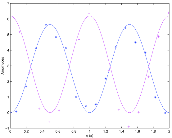
Figure 1: The graph of the amplitudes of C1 and C3 vs. $\varphi=Jt/\sqrt{2}$. The amplitudes have arbitrary units. The data for C1 are marked by ”+”, and are fitted as $A_{1}\cos^{2}\varphi$; the data for C3 are marked by ” * ”, and are fitted as $A_{3}\sin^{2}\varphi$, where $A_{1}=6.20$ and $A_{3}=5.65$.

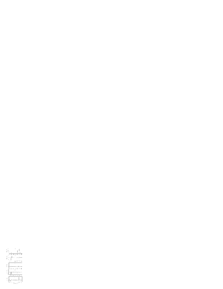
Figure 2: The NMR spectra for the implementation of the perfect state transfer when the initial state is $\sigma_{y}^{1}$. When $\varphi=0$, $\varphi=\pi/2$, $\varphi=\pi$, $\varphi=3\pi/2$, and $\varphi=2\pi$, the system lies in $\sigma_{y}^{1}$ (the initial state), $-\sigma_{z}^{1}\sigma_{z}^{2}\sigma_{y}^{3}$, $\sigma_{y}^{1}$, $-\sigma_{z}^{1}\sigma_{z}^{2}\sigma_{y}^{3}$, and $\sigma_{y}^{1}$, shown as Figs. (a-e), respectively. Fig. (a) is the reference spectrum used to calibrate the phases of the signals in Figs. (b-e).

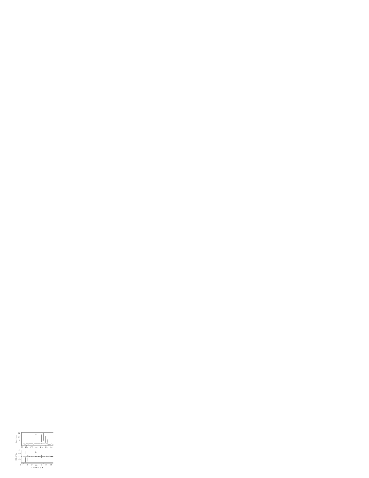
Figure 3: The NMR spectra for the implementation of the perfect state transfer when the initial state is $\sigma_{x}^{1}$. When $\varphi=0$ and $\varphi=\pi/2$, the system lies in $\sigma_{x}^{1}$ (the initial state) and $-\sigma_{z}^{1}\sigma_{z}^{2}\sigma_{x}^{3}$ shown as Figs. (a-b), respectively. Fig. (a) is the reference spectrum. There is a $\pi/2$ phase difference between the signals in Fig. (a) and Fig. 2(a).

References

- (1) R. P. Feynman, Int. J. Theor. Phys, 21, 467(1982)
- (2) D. Deutsch, Proc. R. Soc. A, 400, 97(1985)
- (3) D. Deutsch, Proc. R. Soc. A, 425, 73(1989)
- (4) A. Steane, Rep. Prog. Phys, 61, 117(1998)
- (5) D. Deutsch, A. Barenco, and A. Ekert, Proc. R. Soc, A, 449, 669(1995); Preprint quant-ph/9505018
- (6) M. J. Bremner, C. M. Dawson, J. L.Dodd, A. Gilchrist, A. W. Harrow, D. Mortimer, M. A. Nielsen and T. J. Osborne Phys. Rev. Lett, 89 247902(2002)
- (7) M. A. Nielsen and I. L. Chuang, Quantum Computation and Quantum Information (Cambridge: Cambridge University Press(2000))
- (8) A. Barenco , C. H. Bennett, R. Cleve, D. P. DiVincenzo, N. Margolus, P. Shor, T. Sleator ,J. A. Smolin and H. Weinfurter, Phys. Rev. A 52, 3457(1995)
- (9) R. Cleve, A. Ekert, C. Macchiavello and M. Mosca, Proc. R. Soc. A, 454 339(1998)
- (10) P. W. Shor, Polynomial-Time Algorithms for prime factorization and discrete logarithms on a quantum computer, Proc. 35th Annual Symp. on Foundations of Computer Science, Santa Fe, NM: IEEE Computer Society Press, Nov. 20-22(1994); quant-ph/9508027
- (11) L. K. Grover, Phys. Rev. Lett, 79, 325 (1997)
- (12) L. M. K. Vandersypen, and I. L. Chuang, 76, Rev. Mod. Phys, 76, 1037(2004)
- (13) D. Loss and D. P. DiVincenzo, Phys. Rev. A, 57,120(1998)
- (14) G. Burkard, D. Loss, D. P. DiVincenzo, Phys. Rev. B 59, 2070(1999)
- (15) B. E. Kane, Nature, 393, 133-137(1998)
- (16) T. D. Ladd, J. R. Goldman, F. Yamaguchi, Y. Yamamoto, E. Abe, and K. M. Itoh, Phys. Rev. lett, 89, 017901(2002)
- (17) H. G. Krojanski, and D. Suter, Phys. Rev. Lett, 93, 090501(2004)
- (18) R. Vrijen, E. Yablonovitch, K. Wang, H. W. Jiang, A. Balandin, V. Roychowdhury, T. Mor, and D. DiVincenzo, Phys. Rev. A, 62, 012306(2000)
- (19) J. I. Cirac, and P. Zoller, Phys. Rev. Lett, 74, 4091(1995)
- (20) J. I. Cirac, and P. Zoller, Nature, 404, 579(2000)
- (21) Y. Makhlin, G. Schön, and A. Shnirman, Rev. Mod. Phys, 73, 357(2001)
- (22) M. H. Devoret, A. Wallraff, and J. M. Martinis, cond-mat/ 0411174
- (23) T. Sleator, and H. Weinfurter, Phys. Rev. Lett, 74, 4087-4090(1995)
- (24) V. Giovannetti, D. Vitali, P. Tombesi, A. Ekert, quant-ph/0004107
- (25) F. Yamaguchi, P. Milman, M. Brune, J. M. Raimond, and S. Haroche, Phys. Rev. A, 66, 010302(R) (2002)
- (26) S.-B. Zheng, Phys. Rev. A 70, 052320 (2004)
- (27) L. M. K. Vandersypen, M. Steffen, G. Breyta, C. S. Yannoni, M. H. Sherwood, and I. L. Chuang, Nature, 414, 883(2001)
- (28) N. Boulant, L. Viola, E. M. Fortunato, D. G. Cory, preprint, quant-ph/0409193
- (29) C. Miquel, J. P. Paz, M. Saraceno, E. Knill, R. Laflamme, and C. Negrevergne, Nature, 418, 59(2002)
- (30) S. Lloyd, Nature, 273, 1073(1996)
- (31) B. M. Boghosian, and W. Taylor IV, Physica D, 120, 30(1998)
- (32) S. Somaroo, C. H. Tseng, T. F. Havel, R. Laflamme, and D. G. Cory, Phys. Rev. Lett, 82, 5381(1999)
- (33) J.-F. Du, P. Zou, D. K. L. Oi, X. -H. Peng, L. C. Kwek, C. H. Oh, A. Ekert, preprint quant-ph/0411180
- (34) J.- F. Du, T. Durt, P. Zou, H. Li, L. C. Kwek, C. H. Lai, C. H. Oh, and A. Ekert, Phys. Rev. Lett, 94, 040505 (2005)
- (35) J.-F. Zhang, G. L. Long, Z.-W. Deng, W.-Z. Liu, and Z.-H Lu, Phys. Rev. A, 70, 062322(2004)
- (36) J.-F. Zhang, W.-Z. Liu, Z.-W. Deng, Z.-H Lu and G. L. Long, J. Opt. B, 7 22 C28(2005)
- (37) X.-H. Peng, J.-F Du, and D. Suter, Phys. Rev. A, 71, 012307 (2005)
- (38) C. Negrevergne, R. Somma, G. Ortiz, E. Knill, R. Laflamme, preprint, quant-ph/0410106
- (39) X.-D. Yang, A.-M. Wang, F. Xu, J.-F Du, preprint, quant-ph/0410143
- (40) D. Gunlycke, V. M. Kendon, and V. Vedral, Phys. Rev. A, 64, 042302(2001)
- (41) D. P. DiVincenzo, D. Bacon, J. Kempe, G. Burkard, and K. B. Whaley, Nature, 408, 339(2000)
- (42) D. Bacon, J. Kempe, D. A. Lidar, and K. B. Whaley, Phys. Rev. Lett. 85, 1758 C1761 (2000)
- (43) E. Knill, Nature, 434,39(2005)
- (44) M. Christandl, N. Datta, A. Ekert, and A. J. Landahl, Phys. Rev. Lett, 92, 187902(2004); the extended version: preprint quant-ph/0411020
- (45) Z. L. Madi, R. Brüschweiler, and R. R. Ernst, J. Chem. Phys, 109, 10603(1998)
- (46) M. C. Arnesen, S. Bose, and V. Vedral, Phys. Rev. Lett, 87, 017901(2001)
- (47) L. Zhou, H. S. Song, Y. Q. Guo, and C. Li, Phys. Rev. A, 68, 024301(2003)
- (48) J. P. Keating and F. Mezzadri, Phys. Rev. Lett, 94, 050501(2005)
- (49) M. Mohseni, and D. A. Lidar, Phys. Rev. Lett, 94, 040507 (2005)
- (50) S.-J. Gu, H. Li, Y.-Q. Li, and H.-Q. Lin, Phys. Rev. A, 70, 052302(2004)
- (51) S.-J. Gu, H.-Q. Lin, and Y.-Q. Li, Phys. Rev. A, 68, 042330 (2003)
- (52) X.-G. Wang, Phys. Rev. E, 69, 066118 (2004)
- (53) X.-G. Wang, Phys. Rev. A, 66, 044305(2002)
- (54) D. G. Cory, M. D. Price, and T. F. Havel, Physical D, 120, 82(1998)
- (55) R. R. Ernst, G. Bodenhausen and A. Wokaum, Principles of nuclear magnegtic resonance in one and two dimensions, (Oxford University Press, Oxford, 1987).
- (56) J. -F. Du, H. Li, X. -D. Xu, M. -J. Shi, J. -H. Wu, X. -Y. Zhou, R. -D. Han, Phys. Rev. A 67, 042316(2003)
- (57) N.Linden, . Kupe, and R. Freeman, Chem. Phys. Lett, 311, 321(1999)
- (58) N. Linden, B. Herv, R. J. Carbajo, and R. Freeman, Chem. Phys. Lett, 305, 28(1999)
- (59) H. Geen, and R. Freeman, J. Magn. Reson. 93, 93 (1991)
- (60) C. H. Tseng, S. Somaroo, Y. Sharf, E. Knill, R. Laflamme, T. F. Havel, and D. G. Cory, Phys. Rev. A, 61, 012302(1999)