Analytic pulse design for selective population transfer in many-level quantum systems: optimizing the pulse duration

Abstract

In the previous paper on this topic it was shown how, for a pulse of arbitrary shape and duration, the drive frequency can be analytically optimized to maximize the amplitude of the population oscillations between the selected two levels in a general many level quantum system. It was shown how the standard Rabi theory can be extended beyond the simple two-level systems. Now, in order to achieve the quickest and as complete as possible population transfer between two pre-selected levels, driving pulse should be tailored so that it produces only a single half-oscillation of the population. In this paper, this second (and final) step towards the controlled population transfer using modified (i.e. many level system) Rabi oscillations is discussed. The results presented herein can be regarded as an extension of the standard $\pi$-pulse theory - also strictly valid only in the two level systems - to the coherently driven population oscillations in general many level systems.

I Introduction

During the past 20 years a number of methods has been devised for state selective preparation and manipulation of discrete-level quantum systems paramonov1983 ; chelkowski1990 ; kaluza1993 ; bergmann1998 ; rabitz2003 . However, simple population oscillations, induced by a resonant driving pulse have received negligible attention as a prospective population manipulation method. This might be attributed to two reasons. The first is that Rabi theory is based on the rotating wave approximation (RWA), and all attempts to generalize it without RWA (e.g. shariar2002.1 ; barata2000 ; fujii2003 ) are mathematically very involved. The second is that no attempt has been made to analytically generalize the original Rabi theory beyond the two-level systems.

In this paper an analytic extension of Rabi theory to transitions in many-level systems is presented. The aim is to ’design’ a driving pulse of the form:

$$F(t)=F_{\rm 0}\;m(t)\;\cos{(\omega(t)\;t)}$$ (1)

by establishing analytical optimization relations between its parameters: maximum pulse amplitude $F_{0}$, pulse envelope shape $m(t)$, and time dependent carrier frequency $\omega(t)$. The goal of this enterprize is twofold: the first is to achieve as complete as possible transfer of population between two selected states of the system; the second is to make this transfer as rapid as possible. These two requirements, however, are conflicting: population transfer can be accelerated by using a more intense drive, but at the same time a stronger drive increases involvement of remaining system levels in population dynamics hence deteriorating population transfer between a selected pair of levels.

In the previous paper on this topic bonacci2003.2 it was shown how, for a pulse of arbitrary shape and duration, the drive frequency can be analytically optimized to maximize the amplitude of the population oscillations between the selected two levels in a general many level quantum system. It was shown how the standard Rabi theory can be extended beyond the simple two-level systems. Now, in order to achieve the quickest and as complete as possible population transfer between two pre-selected levels, driving pulse should be tailored so that it produces only a single half-oscillation of the population. In this paper, this second (and final) step towards the controlled population transfer using modified (i.e. many level system) Rabi oscillations is discussed. The results presented herein can be regarded as an extension of the standard $\pi$-pulse theory (see e.g. holthaus1994 ) - also strictly valid only in the two level systems - to the coherently driven population oscillations in general many level systems.

II Theoretical analysis

All the calculations in this section are done in a system of units in which $\hbar=1$.

II.1 Calculation setup

A quantum system with N discrete stationary levels with energies $E_{i}\ (i=1,...,N)$ is considered. The system is driven by a time dependent perturbation given in Eq. (1). In the interaction picture, the dynamics of the system obeys the Schroedinger equation:

$$\frac{d}{dt}\mathbf{a}(t)=-i\hat{\mathbf{V}}(t)\mathbf{a}(t),$$ (2)

where $\mathbf{a}(t)$ is a vector of time-dependent expansion coefficients $a_{1}(t),...,a_{N}(t)$. The N$\times$N Matrix $\hat{\mathbf{V}}(t)$ describes interaction between the system and perturbation. Explicitly, its elements are given by:

$$V_{ij}(t)\equiv\frac{F_{0}\mu_{ij}}{2}m(t)(e^{is_{ij}(\omega(t)-\omega_{ij})t}+e^{-is_{ij}(\omega(t)+\omega_{ij})\;t}).$$ (3)

$\mu_{ij}$ is transition moment between the i-th and the j-th levels induced by the perturbation. $s_{ij}\equiv sign(E_{i}-E_{j})$ and $\omega_{ij}\equiv|E_{i}-E_{j}|$ are respectively the sign and the magnitude of the resonant frequency for the transition between the i-th and the j-th level.

The aim is to induce population transfer between two arbitrarily selected levels, designated by $\alpha$ and $\beta$, directly coupled by the perturbation (i.e. such that $\mu_{\alpha\beta}\neq 0$). To simplify equations, the time variable t is re-scaled to $\tau$, with transformation between the two given by:

$$d\tau\equiv\frac{F_{0}\mu_{\alpha\beta}}{2}m(t)dt.$$ (4)

Then with following substitutions:

$$f_{ij}(\tau) \equiv s_{ij}\frac{2}{F_{0}\mu_{\alpha\beta}}(\omega(t)-\omega_{ij})$$ (5)

$$g_{ij}(\tau) \equiv s_{ij}\frac{2}{F_{0}\mu_{\alpha\beta}}(\omega(t)+\omega_{ij})$$ (6)

$$x(\tau) \equiv \frac{F_{0}\mu_{\alpha\beta}}{2}t(\tau)$$ (7)

$$R_{ij} \equiv \frac{\mu_{ij}}{\mu_{\alpha\beta}}$$ (8)

Eq. (2) transforms into:

$$\frac{d}{d\tau}\mathbf{a}(\tau)=-i\hat{\mathbf{W}}(\tau)\mathbf{a}(\tau),$$ (9)

where:

$$W_{ij}(\tau)\equiv R_{ij}(e^{if_{ij}(\tau)x(\tau)}+e^{-ig_{ij}(\tau)x(\tau)}).$$ (10)

Initial conditions for the problem of selective population transfer comprise complete population initially (at $t=\tau=0$) contained in only one of the selected levels, either $\alpha$ or $\beta$. The other selected level, as well as all the remaining N-2 ’perturbing’ levels of the system are unpopulated at this time.

Population evolution $\Pi_{i}(t)$ of the i-th level is determined from $\Pi_{i}(t)=|a_{i}(t)|^{2}$.

II.2 Rabi-like population transfer in a three level system

It was demonstrated in the previous paper on this topic bonacci2003.2 that the analytical extension of the Rabi oscillations theory beyond two-level systems is anchored in the analysis of the simplest of the ’many-level’ systems - a three level one. Hence, in this section the impact of the single additional level on the population transfer period is discussed: beyond the ’selected’ levels $\alpha$ and $\beta$, the system now contains one additional ’perturbing’ level, designated with index p. The only requirements on the system internal structure are that $\mu_{\alpha\beta},\mu_{\beta p}\neq 0$ and $\mu_{\alpha p}=0$. While the first two requirements are necessary, the last one does not reduce the generality of the final results to any significant extent and is introduced for calculational convenience exclusively.

For the observed three-level system, the dynamical equation (9) reduces to:

$$\frac{d}{d\tau}\begin{bmatrix}a_{\alpha}(\tau)\\ a_{\beta}(\tau)\\ a_{p}(\tau)\\ \end{bmatrix} =$$ (11)

$$- i \begin{bmatrix}0&e^{if_{\alpha\beta}(\tau)x(\tau)}+e^{-ig_{\alpha\beta}(\tau)x(\tau)}&0\\ e^{-if_{\alpha\beta}(\tau)x(\tau)}+e^{ig_{\alpha\beta}(\tau)x(\tau)}&0&R_{\beta p}(e^{-if_{\beta p}(\tau)x(\tau)}+e^{ig_{\beta p}(\tau)x(\tau)})\\ 0&R_{\beta p}(e^{if_{\beta p}(\tau)x(\tau)}+e^{-ig_{\beta p}(\tau)x(\tau)})&0\\ \end{bmatrix}\begin{bmatrix}a_{\alpha}(\tau)\\ a_{\beta}(\tau)\\ a_{p}(\tau)\\ \end{bmatrix}$$

II.2.1 Recapitulation: minimizing the impact of the perturbing level

As it was shown in bonacci2003.2 , Eq. (11), when the driving frequency is near the resonant value for the transition $\alpha\leftrightarrow\beta$, the following expression can be obtained for the population dynamics of level p:

$$a_{p}(\tau)\approx-a_{\beta}(\tau)\Big{(}\sigma_{\beta p}\frac{m(t(\tau))}{1-\Delta_{\beta p}(\tau)}\Big{)}\;e^{if_{\beta p}(\tau)x(\tau)}$$ (12)

where

$$\sigma_{\beta p}\equiv\frac{F_{0}\mu_{\beta p}}{2(\omega_{\alpha\beta}-\omega_{\beta p})}\,$$

$$\Delta_{\beta p}(\tau)\equiv\frac{\omega(\tau)-\omega_{\alpha\beta}}{\omega_{\beta p}-\omega_{\alpha\beta}}\ .$$ (13)

Put in words, with the conditions mentioned, the dynamics of the level p parametrically depends on the dynamics of the level $\beta$ to which it is coupled. The relation between the amplitudes of the population oscillations for levels p and $\beta$ follows directly from the above expression:

$$\Pi_{p} \approx \epsilon_{\beta p}(\tau)\Pi_{\beta}(\tau)$$ (14)

where:

$$\epsilon_{\beta p}(\tau)\equiv\Big{(}\sigma_{\beta p}\frac{m(t(\tau))}{1-\Delta_{\beta p}(\tau)}\Big{)}^{2}\ .$$ (15)

Note that, as $\Delta_{\beta p}(\tau)$ is generally very small and $|m(\tau)|\leq 1$, that parameter $\sigma_{\beta p}$ actually determines the effective strength of applied perturbation: if $\sigma_{\beta p}^{2}<<1$, then dynamical impact of level p is negligible and perturbation may be considered weak; if $\sigma_{\beta p}^{2}\sim 1$, perturbation is very strong.

Further, the requirement of the minimization of the dynamical impact of the perturbing level p on the transition $\alpha\leftrightarrow\beta$ leads to the following equation for the optimized dynamics of the ($\alpha$,$\beta$) subsystem:

$$\frac{d}{d\tau}\begin{bmatrix}b_{\alpha}(\tau)\cr b_{\beta}(\tau)\end{bmatrix}=-i\begin{bmatrix}0&1\cr 1&0\cr\end{bmatrix}\begin{bmatrix}b_{\alpha}(\tau)\cr b_{\beta}(\tau)\end{bmatrix}$$ (16)

where the two-level state vector $\big{(}b_{\alpha}(\tau),b_{\beta}(\tau)\big{)}$ is merely the unitary transformed vector of the subsystem ($\alpha$,$\beta$):

$$\begin{bmatrix}b_{\alpha}(\tau)\\ b_{\beta}(\tau)\\ \end{bmatrix}=e^{-i\hat{\mathbf{\Lambda}}(\tau)}\begin{bmatrix}a_{\alpha}(\tau)\\ a_{\beta}(\tau)\\ \end{bmatrix}$$ (17)

Note that the precise form of the real transformation matrix $\hat{\mathbf{\Lambda}}(\tau)$ is irrelevant here as it has no impact on the population dynamics.

The optimization procedure produces the analytic expression for the chirp of the driving frequency, which in the lowest order of approximation (suitable for all but the most intensive perturbations) amounts:

$$\omega(t)=\omega_{\alpha\beta}+(s_{\beta\alpha}s_{\beta p})(\omega_{\beta p}-\omega_{\alpha\beta})\frac{2\omega_{\beta p}}{\omega_{\alpha\beta}+\omega_{\beta p}}\sigma_{\beta p}^{2}\frac{1}{t}\int_{0}^{t}\big{(}m(t^{\prime})\big{)}^{2}dt^{\prime}$$ (18)

and from the Eq (16) it is found that the time $\Theta$ required for a single population transfer between levels $\alpha$ and $\beta$, determined from the fundamental relation of the $\pi$-pulse theory:

$$\int_{0}^{\Theta}d\tau=\frac{\pi}{2}$$ (19)

equals (in units of $\tau$):

$$\Theta=\frac{\pi}{2}$$ (20)

As was shown in bonacci2003.2 , the ’exact’ numerical solution to the Eq. (11) indeed maximizes the population oscillations in the $\alpha-\beta$ subsystem. However, as will be discussed below, the predicted value for the period of the population oscillations (Eq. (20)) is somewhat smaller than the correct one, with the discrepancy increasing with the increasing population leak to the level p. In the following section this issue is resolved and the corrected analytical expression for determination of the population transfer (or oscillation) period is obtained.

II.2.2 Patching the population conservation of the total system

To start the following discussion, notice that the optimized solution for the population transfer between levels $\alpha$ and $\beta$ (described by the Eq. (16)) is unfortunately too good to be true. Namely, its serious drawback lays in the fact that the leak of the population from the ($\alpha$,$\beta$) subsystem into the perturbing level p goes by completely unnoticed!

Formally, the root of the problem hides in the fact that the mathematical trick which enabled decoupling of the level p dynamics from the rest of the system (i.e. the step between Eq.(18) and Eq.(19) in bonacci2003.2 ) destroys the unitarity of the full dynamical equation for the three level system, Eq.(11). The consequence is that the dynamical equation for the $\alpha-\beta$ subsystem, Eq.(16) itself claims to be unitary, keeping the population of that subsystem fully conserved. This is clearly impossible, as level p does indeed capture some population - the exact amount given by Eq.(14).

This malfunction caused by the decoupling procedure unfortunately cannot be remedied within the decoupling procedure itself - the patch has to be provided by an independent approach. To do this, the following argument is used: since it is the equation for the dynamics of level $\beta$ that changes due to the decoupling procedure and consequently causes the breakdown of the population conservation, it is only the dynamical equation for the level $\beta$ that has to be modified; then, as the dynamics of the level $\beta$ is governed by the elements in the lower row of the dynamical matrix in Eq.(16), a particular ansatz intervention precisely into these elements might help rectify the overall population dynamics of the whole three level system. Hence, the correction is sought in the following form:

$$\frac{d}{d\tau}\begin{bmatrix}b_{\alpha}(\tau)\\ b_{\beta}(\tau)\\ \end{bmatrix}=-i\begin{bmatrix}0&1\\ \zeta(\tau)&i\xi(\tau)\\ \end{bmatrix}\begin{bmatrix}b_{\alpha}(\tau)\\ b_{\beta}(\tau)\\ \end{bmatrix}$$ (21)

where $\zeta[\tau]$ and $\xi[\tau]$ are real non-negative functions. Such an ansatz does not interfere with the phase-fitting effect of the driving frequency optimization and Eq. (18) - forged by the decoupling procedure - which maximizes the population oscillations in the $\alpha-\beta$ subsystem, is left unharmed. Instead, it merely enables phase-independent modification of the amplitudes of $\alpha$ and $\beta$ populations.

Expressing requirement of population conservation in the total three-level system as:

$$d|b_{\alpha}(\tau)|^{2}+d|b_{\beta}(\tau)|^{2}+d|b_{p}(\tau)|^{2}=0\ ,$$ (22)

splitting the phase and amplitude contributions of the three wave function projections on the three stationary states:

$$b_{\alpha}(\tau) \equiv B_{\alpha}(\tau)e^{i\phi_{\alpha}(\tau)}\ ,$$

$$b_{\beta}(\tau) \equiv B_{\beta}(\tau)e^{i\phi_{\beta}(\tau)}\ ,$$ (23)

$$b_{p}(\tau) \equiv B_{p}(\tau)e^{i\phi_{p}(\tau)}\ ,$$

and using the known relation between the populations of levels $\beta$ and p, Eq.(14), the following result is obtained:

$$B_{\alpha}(\tau)\;dB_{\alpha}+(1+\epsilon_{\beta p}(\tau))B_{\beta}(\tau)\;dB_{\beta}+\frac{1}{2}B_{\beta}(\tau)^{2}\;d\epsilon_{\beta p}=0\ .$$ (24)

Now the corrected equation for the $\alpha-\beta$ subsystem, Eq.(21), can be used to eliminate $dB_{\alpha}$ and $dB_{\beta}$ and introduce $\zeta[\tau]$ and $\xi[\tau]$ in their stead:

$$dB_{\alpha} = -iB_{\beta}\;Im\big{(}e^{i(\phi_{\beta}(\tau)-\phi_{\alpha}(\tau))}\big{)}\;d{\tau}\ ,$$

$$dB_{\beta} = -i\Big{(}\zeta(\tau)\;B_{\alpha}(\tau)\;Im\big{(}e^{-i(\phi_{\beta}(\tau)-\phi_{\alpha}(\tau))}\big{)}+\xi(\tau)\;B_{\beta}(\tau)Im\big{(}e^{-i\phi_{\beta}(\tau)}\big{)}\Big{)}\;d{\tau}\ .$$ (25)

Finally, taking together Eq.(24) and Eq.(II.2.2) it is found that:

$$B_{\alpha}(\tau)\Big{(}\zeta(\tau)-\frac{1}{1+\epsilon_{\beta p}(\tau)}\Big{)}\ sin\big{(}\phi_{\beta}(\tau)-\phi_{\alpha}(\tau)\big{)}+B_{\beta}(\tau)\Big{(}\xi(\tau)+\frac{d}{d\tau}\ln\big{(}1+\epsilon_{\beta p}(\tau)\big{)}^{\frac{1}{2}}\Big{)}sin\big{(}\phi_{\beta}(\tau)\big{)}=0.$$ (26)

Since for population oscillations $B_{\beta}$ and $B_{\alpha}$ are $180^{o}$ out of phase, this condition can be satisfied only if:

$$\zeta(\tau) = \frac{1}{1+\epsilon_{\beta p}(\tau)}\ ,$$

$$\xi(\tau) = -\frac{d}{d\tau}\ln\big{(}1+\epsilon_{\beta p}(\tau)\big{)}^{\frac{1}{2}}\ .$$ (27)

II.2.3 Population oscillation period modified

Hence, the correct dynamical equation for the $\alpha-\beta$ subsystem which both maximizes the population oscillation amplitudes of these two levels as well as properly conserves the overall population of the three-level ($\alpha-\beta-p$) system is:

$$\frac{d}{d\tau}\begin{bmatrix}b_{\alpha}(\tau)\\ b_{\beta}(\tau)\\ \end{bmatrix}=-i\begin{bmatrix}0&1\\ \frac{1}{1+\epsilon_{\beta p}(\tau)}&-i\frac{d}{d\tau}\ln\big{(}1+\epsilon_{\beta p}(\tau)\big{)}^{\frac{1}{2}}\\ \end{bmatrix}\begin{bmatrix}b_{\alpha}(\tau)\\ b_{\beta}(\tau)\\ \end{bmatrix}\ .$$ (28)

A simple extension of this result to the general many-level system (in which level $\alpha$ also has some perturbing levels - jointly designated by q - attached to it) yields the total corrected dynamical equation for such a system:

$$\frac{d}{d\tau}\begin{bmatrix}b_{\alpha}(\tau)\\ b_{\beta}(\tau)\\ \end{bmatrix}=-i\begin{bmatrix}-i\frac{d}{d\tau}\ln\big{(}1+\epsilon_{\alpha q}(\tau)\big{)}^{\frac{1}{2}}&\frac{1}{1+\epsilon_{\alpha q}(\tau)}\\ \frac{1}{1+\epsilon_{\beta p}(\tau)}&-i\frac{d}{d\tau}\ln\big{(}1+\epsilon_{\beta p}(\tau)\big{)}^{\frac{1}{2}}\\ \end{bmatrix}\begin{bmatrix}b_{\alpha}(\tau)\\ b_{\beta}(\tau)\\ \end{bmatrix}\ .$$ (29)

Now to finalize the calculation of the corrected population transfer period the following procedure is administered. First, the time variable is transformed $\tau\rightarrow\varphi$ according to:

$$d\tau=\kappa(\varphi)d\varphi$$ (30)

The goal of this variable transformation is to produce, in the new time variable $\varphi$, the closed dynamical equations for $b_{\alpha}(\varphi)$ and $b_{\beta}(\varphi)$ describing the dynamics which is as close as possible to the simple harmonic oscillation. Second, and to that end, the transformation Eq.(30) is introduced into Eq.(29), the resulting relation is differentiated with respect to $\varphi$ and all but the lowest order terms in the small parameters $\epsilon_{\alpha q}(\tau)$ and $\epsilon_{\beta p}(\tau)$ are kept. Hence the following result is established:

$$\frac{d^{2}b_{\alpha}(\varphi)}{d\varphi^{2}}+\frac{1}{2}\frac{d}{d\varphi}\Big{(}\ln\frac{\big{(}1+\epsilon_{\alpha q}(\varphi)\big{)}^{3}\big{(}1+\epsilon_{\beta p}(\varphi)\big{)}}{\kappa^{2}}\Big{)}\;\frac{db_{\alpha}(\varphi)}{d\varphi}+\frac{\kappa^{2}}{\big{(}1+\epsilon_{\alpha q}(\varphi)\big{)}\big{(}1+\epsilon_{\beta p}(\varphi)\big{)}}b_{\alpha}(\varphi)=0$$

$$\frac{d^{2}b_{\beta}(\varphi)}{d\varphi^{2}}+\frac{1}{2}\frac{d}{d\varphi}\Big{(}\ln\frac{\big{(}1+\epsilon_{\alpha q}(\varphi)\big{)}\big{(}1+\epsilon_{\beta p}(\varphi)\big{)}^{3}}{\kappa^{2}}\Big{)}\;\frac{db_{\beta}(\varphi)}{d\varphi}+\frac{\kappa^{2}}{\big{(}1+\epsilon_{\alpha q}(\varphi)\big{)}\big{(}1+\epsilon_{\beta p}(\varphi)\big{)}}b_{\beta}(\varphi)=0$$ (31)

In the third and final step, the appropriate value of the free parameter $\kappa(\varphi)$ is selected:

$$\kappa(\varphi)^{2}\equiv\big{(}1+\epsilon_{\alpha q}(\varphi)\big{)}\big{(}1+\epsilon_{\beta p}(\varphi)\big{)}$$ (32)

which transforms Eq.(II.2.3) into:

$$\frac{d^{2}b_{\alpha}(\varphi)}{d\varphi^{2}}+\frac{d}{d\varphi}(\ln(1+\epsilon_{\alpha q}(\varphi)))\frac{db_{\alpha}(\varphi)}{d\varphi}+b_{\alpha}(\varphi)=0$$

$$\frac{d^{2}b_{\beta}(\varphi)}{d\varphi^{2}}+\frac{d}{d\varphi}(\ln(1+\epsilon_{\beta p}(\varphi)))\frac{db_{\beta}(\varphi)}{d\varphi}+b_{\beta}(\varphi)=0$$ (33)

Both these equations are similar to the damped oscillator equation. For negligible damping ($\epsilon_{\alpha q}(\varphi),\epsilon_{\beta p}(\varphi)<<1$), they reduce to the harmonic oscillator equations, in which case the population transfer time of $\pi/2$ is obtained in the variable $\varphi$. In the the original time coordinate, $\tau$, the corrected time $\Theta$ required for a single population transfer between the levels $\alpha$ and $\beta$ is then obtained from:

$$\int_{0}^{\Theta}\frac{d\tau}{\sqrt{(1+\epsilon_{\alpha q}(\tau))(1+\epsilon_{\beta p}(\tau))}}=\frac{\pi}{2}$$ (34)

Note the difference between this result, and the result in Eq. (19) obtained from the standard $\pi$-pulse theory: in the lowest order approximation, the corrected population transfer time is shorter then the one obtained from Eq. (19) by an order of $\frac{1}{2}(\epsilon_{\alpha q}(\tau)+\epsilon_{\beta p}(\tau))$.

On the other hand, taking into consideration the damping factor in the Eq.(II.2.3), approximating:

$$\frac{d}{d\varphi}\ln(1+\epsilon_{\alpha q,\beta p}(\varphi))\approx\frac{d}{d\varphi}\epsilon_{\alpha q,\beta p}(\varphi)$$ (35)

and using the damped oscillator theory Kent1996 (p.246), an increase in the damping (expressed as an increase in $\epsilon_{\alpha q}(\tau)$ and $\epsilon_{\beta p}(\tau)$) leads to the an increase in the population time transfer by an order of $\frac{1}{2}\frac{d}{d\tau}\epsilon_{\alpha q,\beta p}^{2}(\tau)$. As this correction is an order of magnitude smaller than the correction obtained from Eq.(34), it can be neglected for all practical purposes. Furthermore, the additional corrections to the transfer period due to the neglected higher order elements in the Eq.(II.2.3) are of the same order of magnitude as this correction due to the first derivative component, and as they are impossible to obtain analytically, the value of this whole second order correction for the case of strong perturbations is somewhat shaky. However, this is not an issue, as the whole optimization theory developed in bonacci2003.2 - and on whose applicability the results of the above analysis hinge - assumes rather modest perturbations, and is not even expected to work properly for the extreme values.

III Numerical simulations

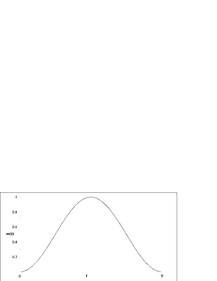
Figure 1: In all of the numerical examples the same pulse form was used - $m(t)=\sin(\Omega t)^{2}$, but with different values of maximum intensity parameter ($F_{0}$) and different total pulse duration, $T$. The respective values are quoted in each particular example.

In this section, numerical simulations of system dynamics for unoptimized and fully optimized driving pulse of the form of Eq. (1) are presented and compared. Here, unoptimized driving pulse is the one with driving frequency equal to the pure resonant frequency between the two levels selected for population transfer ($\omega(t)=\omega_{\alpha\beta}$) and with pulse duration $T$ determined according to the standard $\pi$-pulse theory relation, Eq.(19). On the other hand, the parameters of the fully optimized pulse are determined from Eq.(18) and Eq.(34).

In all cases, a three-level system is considered, with the following system parameters ($a.u.\equiv atomic\;units$): $\omega_{\beta\alpha}=0.017671\;a.u.$, $s_{\beta\alpha}=1$, $\mu_{\beta\alpha}=0.073\;a.u.$; $\omega_{\beta p}=0.017611\;a.u.$, $s_{\beta p}=-1$, $\mu_{\beta p}=0.098\;a.u.$. These system parameters correspond to the three ro-vibrational levels of the HF molecule in the ground electronic state: $\alpha\equiv(v=0,j=2,m=0)$, $\beta\equiv(v=1,j=1,m=0)$, $p\equiv(v=2,j=2,m=0)$. The pulse shape in all of the examples is $m(t)=\sin(\Omega t)^{2}$ as shown in Fig 1.

III.1 Population oscillations

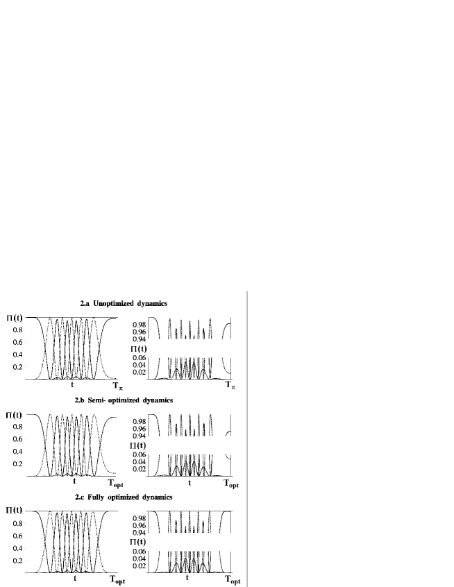
Figure 2: Significance of the total analytical correction (in driving frequency and total pulse duration) for the dynamics of a mildly disturbed system. In all plots, major oscillations are the populations of the two targeted levels ($\alpha$ and $\beta$) whereas the minor oscillations are the population of the perturbing level ($p$). For the value of perturbation strength parameter $\sigma_{\beta p}^{2}=0.05$, the loss of the final unoptimized population transfer amplitude amounts about 2%. Optimization reduces this loss to below 0.05%. The difference between the pulse duration obtained from standard $\pi$-pulse theory and the optimized value is 1.6%. Right hand-side plots present the details from the left hand-side plots.

As was demonstrated in bonacci2003.2 , frequency optimization minimizes the impact of the perturbing levels on the amplitude of the population oscillations. In this subsection, the necessity of the inclusion of additional correction Eq.(34) for the population transfer time - alongside the correction for the driving frequency - will be demonstrated. Also, the validity and the limitations of the analytically obtained expression for this correction will be discussed.

III.1.1 Legitimate perturbation

Fig.2 presents the dynamics of the system subjected to the external drive of limiting intensity, $\sigma_{\beta p}^{2}=0.05$, corresponding to the $F_{0}=2.80534\ast 10^{-4}a.u.$. It is just strong enough to noticeably (albeit not significantly) distort the pure resonant oscillations, but at the same time weak enough so that the theory developed in bonacci2003.2 and further in this paper provides the full and precise quantitative corrections.

Pulse duration determined according to the standard $\pi$-pulse theory expression, Eq.(19) is $T_{\pi}=3077832a.u.$, whereas the optimized one, obtained from Eq.(34) is $T_{opt}=3126029a.u.$. The pulse is aimed at producing five complete population oscillations.

Three cases of dynamics are presented: Fig. 2.a shows the unoptimized dynamics; Fig 2.b shows the ’semi-optimized’ dynamics, with optimized driving frequency, but unoptimized population transfer period; finally, Fig. 2.c shows the fully optimized dynamics. Observe that in the unoptimized case, the population oscillations end somewhat short of the complete cycle, and the initially populated level never achieves complete depopulation. Optimizing only the driving frequency does indeed maximize the population oscillations by inducing the complete depopulation of the initially populated level during oscillations, but at the same time the final population oscillation stops even further from the full cycle than in the unoptimized case. Finally, introducing the population transfer period correction alongside the driving frequency correction yields the required result: complete cycle of maximized population oscillations.

III.1.2 Strong perturbation

Increasing the driving perturbation intensity to somewhat greater value, $\sigma_{\beta p}^{2}=0.25$ ($F_{0}=6.11409\ast 10^{-4}\ a.u.$.), the limitations of the analytical theory clearly emerge. This is shown in Fig. 3: Fig. 3.a - Fig. 3.c respectively show the unoptimized, analytically optimized (according to Eq.(18) and Eq.(34)) and ’manually optimized’ dynamics. The corresponding pulse duration times, aimed at producing three complete population oscillations, are $T_{\pi}=847324\ a.u.$, $T_{opt}=901075\ a.u.$ and $T_{man}=884300\ a.u.$.

Notice that in the analytically optimized case, Fig. 3.b, the initially populated level still fully depopulates, which indicates that even for this rather strong perturbation, the frequency correction Eq.(18) still stands strong. However, the corrected period, although closer to the correct value than in the unoptimized case, is still somewhat removed from the correct value. Unfortunately, this ’optimization error’ cannot be remedied analytically. Remember that the analytical result Eq.(34) is obtained using only the first order approximation (Eq.(II.2.3)) to the full dynamical equations Eq.(29). With perturbation as strong as in this case, the dynamical impact of the neglected elements of that equation begin to show. However, as shown in Fig. 3.c, the full cycle of oscillations can still be produced, but this additional correction to the pulse duration had to be found by hand, using the trial and error method.

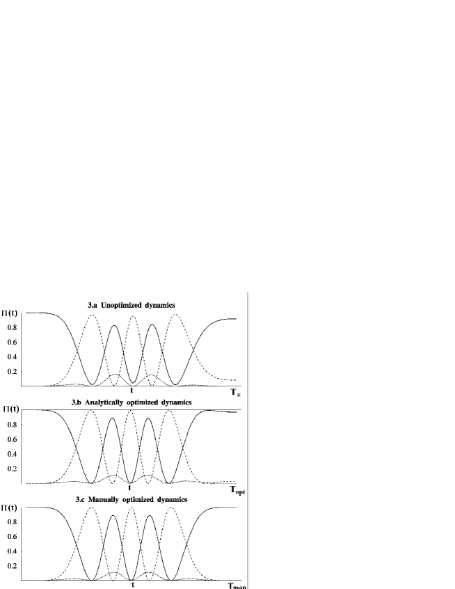
Figure 3: Limitations of the analytical optimization theory. Again, major oscillations are the population of the two targeted levels whereas the minor oscillations are the population of the perturbing level. For the value of perturbation strength parameter is now $\sigma_{\beta p}^{2}=0.25$, which is just beyond the limiting value for the full applicability of the presented optimization procedure. Although the analytical correction improves the final population transfer from 92% to 97% (with pulse duration correction of 6%), the theory presented in this paper cannot account for an additional 1.6% correction in the duration of the pulse that further increases the final population transfer to over 99.99%.

III.2 Population transfer

The two final examples demonstrate the application of the developed optimization theory to the most interesting dynamical case regarding the coherent control: that of the single population transfer between the two targeted levels $\alpha$ and $\beta$. As the validity and the limitations of the whole theory were already explored in the previous two examples, the following examples will only demonstrate the improvements to the population transfer that can be produced using the above results.

III.2.1 Legitimate perturbation

Again as in the previous section, the first example (Fig. 4) presents the dynamics of the system subjected to the external drive of limiting intensity. In this case, the perturbation strength parameter amounts $\sigma_{\beta p}^{2}=0.1$, corresponding to the $F_{0}=4.07606\ast 10^{-4}\ a.u.$. Calculated population transfer times are $T_{\pi}=211831\ a.u.$ and $T_{opt}=218483\ a.u.$.

The unoptimized (dotted line) and the optimized dynamics (solid line) are plotted on the same graph to facilitate the comparison between the two. Only the dynamics of the two target levels is shown - the plot of the perturbing level’s ($p$) dynamics is omitted for the sake of clarity of the overall graph. Although the loss of the population transfer in the unoptimized case is not great, it nevertheless is noticeable. On the other hand, introducing the corrections for pulse frequency and pulse duration clearly improves the population transfer bringing it very close to 100%.

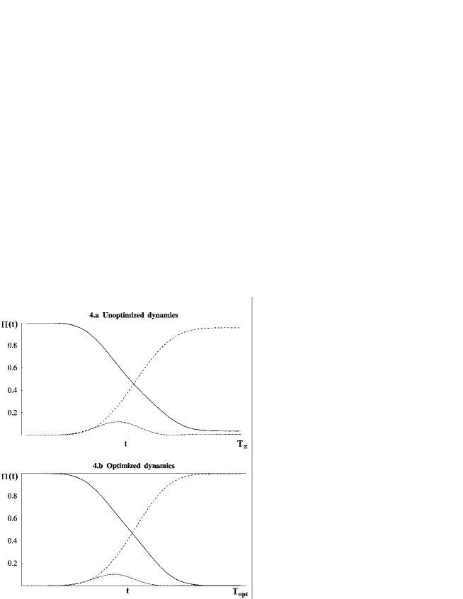
Figure 4: Applicability of the analytical optimization procedure to the maximization of the population transfer. Yet again, major oscillations are the population of the two targeted levels whereas the minor oscillations are the population of the perturbing level. For this limiting value of perturbation strength parameter of $\sigma_{\beta p}^{2}=0.10$, the optimization almost completely eradicates the loss of the population transfer due to the dynamical impact of the perturbing level, increasing the population transfer from 96% to 99.7%. Optimized pulse lasts 3% longer than the one obtained from the standard $\pi$-pulse theory.

III.2.2 Extreme perturbation

The final example - presented in Fig. 5. - is qualitative, rather than quantitative, but even as such it is quite indicative of the overall usefulness of the whole optimization theory. The perturbation is now extreme, with strength parameter $\sigma_{\beta p}^{2}=1$ corresponding to the $F_{0}=1.22282\ast 10^{-3}\ a.u.$. Calculated population transfer times are $T_{\pi}=70610\ a.u.$ and $T_{opt}=82816\ a.u.$.

Again, the unoptimized and the optimized dynamics are plotted on the same graph. Although optimization now clearly does not lead to the complete population transfer, the improvement from the unoptimized dynamics is significant demonstrating that even for this perturbation intensity the developed optimization theory qualitatively works quite nicely.

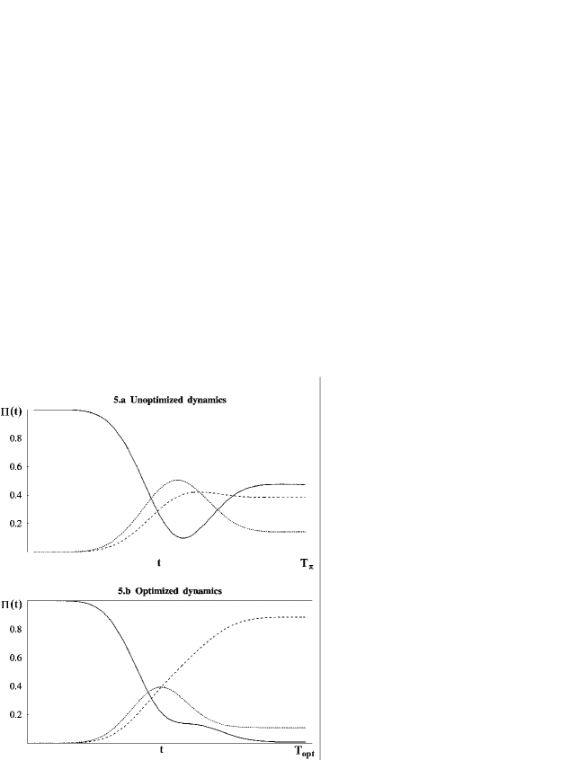
Figure 5: Breakdown of the quantitative optimization, but qualitatively the theory is still applicable. Half way through the pulse, in the unoptimized case now the population of the perturbing level surpasses the population of the initially unpopulated level. Introduction of the optimized driving frequency and pulse duration significantly - although not fully - rectifies the population transfer from below 40% to almost 90%. Optimized pulse is now almost 20% longer then the one obtained from the ordinary $\pi$-pulse theory.

IV Conclusion

The aim of research that led to this paper was to explore the possibility of using ’old fashioned’ and rather simple phenomenon of Rabi oscillations for the controlled manipulation of the population in general many level system. This paper rounds up the topic of analytical optimization of pulse parameters (frequency chirp and pulse duration), opened in the author’s previous work (bonacci2003.2 ) that would lead to maximizing the population transfer between two targeted levels of the system. The theory developed provides the exact quantitative predictions of to what extent the dynamical impact of the remainder of the many level system (beyond the two levels selected for the population transfer) begins to interfere with the targeted population transfer. It also provides the closed (albeit recursive) analytical expressions for the optimization of pulse parameters.

Although the major correction to the population transfer is achieved by optimizing the driving pulse’s frequency chirp (given in bonacci2003.2 ), this paper provides the additional fine tuning by establishing similarly simple analytical expression for the determination of the optimal pulse duration. It demonstrates that the standard formula of the $\pi$-pulse theory, Eq. (19) begins to fail as the perturbation increases to and beyond the well defined limiting value. It also provides some remedy to this failure.

The whole theory presented in bonacci2003.2 and this paper deals with only single laser pulse driving one particular transition in the many level system. The further research currently under way considers the possibility of applying a number of distinct but simultaneous optimized pulses to drive the population through the chain of transitions through the system, hence producing as clean as possible transfer between the two levels not coupled by the single photon transition. The preliminary results indicate that an analytical optimization formula can be developed even for such a case.

References

- (1) G.K.Paramonov, V.A.Savva, Resonance effects in molecule vibrational excitation by picosecond laser pulses, Phys. Lett. A 97A (8) (1983) 340–342.
- (2) S.Chelkowski, A.Bandrauk, P.B.Corkum, Efficient molecular dissociation by chirped ultrashort infrared laser pulse, Phys. Rev. Lett. 65 (19) (1990) 2355–2358.
- (3) M. Kaluza, J.T.Muckerman, P.Gross, H.Rabitz, Optimaly controlled five-laser infrared multiphoton dissociation of hf, J. Chem. Phys. 100 (6) (1993) 4211–4228.
- (4) K.Bergmann, H.Theuer, B.W.Shore, Coherent population transfer among quantum states of atoms and molecules, Rev. Mod. Phys. 70 (1998) 1003–1026.
- (5) H.Rabitz, Shaped laser pulses as reagents, Science (299) (2003) 525–527.
- (6) M.S.Shariar, P.Pradhan, Fundamental limitation on qubit operations due to the bloch-siegert oscillation, Proceedings of the quantum communication, measurement and computing (QCMC’02) Quant-ph/0212121.
- (7) J.C.A.Barata, W.F.Wreszinski, Strong coupling theory of two level atoms in periodic fields, Phys.Rev.Lett. 84 (10) (2000) 2112–2115, quant-ph/9906029.
- (8) K.Fujii, Two-level system and some approximate solutions in the strong coupling regime, quant-ph/0301145 .
- (9) D.Bonacci, S.D.Bosanac, N.Doslic, Analytic pulse design for selective population transfer in many-level quantum systems: maximizing the amplitude of population oscillations, Phys.Rev.A 70 (4) (2003) 043413, quant-ph/0310034.
- (10) M.Holthaus, B.Just, Generalized pulses, Phys. Rev. A 49 (3) (1994) 1950–1960.
- (11) R. Nagle, E. B.Saff, Fundamentals of differential equations and boundary value problems, 2nd Ed., Addison Wesley, 1996.