Quantum computing of delocalization in small-world networks

Abstract

We study a quantum small-world network with disorder and show that the system exhibits a delocalization transition. A quantum algorithm is built up which simulates the evolution operator of the model in a polynomial number of gates for exponential number of vertices in the network. The total computational gain is shown to depend on the parameters of the network and a larger than quadratic speed-up can be reached. We also investigate the robustness of the algorithm in presence of imperfections.

Recently, much attention has been attracted to the study of small-world networks smallworld . They have been shown to describe social and biological networks, Internet connections, airline flights and other complex networks. In such systems, it is possible to go from a given point to any other through only a small number of links. Well-established classical models have been proposed and analyzed by statistical methods. The study of quantum networks with the same property has started only recently, showing that these systems present interesting features related to quantum transport, delocalization chinois ; como2001 and fast diffusion diffusion .

In parallel, the development of quantum information and computation has become more and more important Nielsen . In particular, the study of quantum computers has shown that they can solve certain problems much more efficiently than any classical device. Celebrated quantum algorithms have been built for the factorization of large numbers with exponential efficiency shor , and for search in an unstructured database with a quadratic speed-up grover . As first envisioned by Feynman in the 1980’s, the simulation of complex quantum systems has also been shown to be more efficient on a quantum computer Nielsen .

Here we study a quantum small-world network with disorder. We demonstrate the existence of a delocalization transition and investigate its dependence on disorder strength, number of links and system size. We then build a quantum algorithm to simulate such a network on a quantum computer, and show that its efficiency significantly overcomes classical computations. The algorithm is robust with respect to errors.

We consider a circular graph with $N=2^{n_{r}}$ vertices. Each vertex is linked with its two nearest-neighbors. To this graph, $pN$ shortcut links (connecting $2pN$ vertices) are added between random pairs of vertices (see an example in the inset of Fig.1) footnote . A quantized version of this system with on-site disorder can be described by the $N\times N$ Hamiltonian matrix $H=H_{0}+H_{1}+H_{2}$. The first two terms give a one-dimensional tight-binding Anderson model well-known in solid state physics mirlin . The diagonal matrix with entries $(H_{0})_{ij}=\epsilon_{i}\delta_{i,j}$ describes on-site disorder; $\delta_{i,j}$ denote Kronecker symbols, and $\epsilon_{i}$ are independent random numbers whose distribution is a Gaussian with zero mean and width $W$ (the Gaussian is truncated at large values). The matrix $(H_{1})_{ij}=V(\delta_{i,j+1}+\delta_{i+1,j})$ describes the links between nearest-neighbors, and $(H_{2})_{ij}=\sum_{k=1}^{M}V(\delta_{i,i_{k}}\delta_{j,j_{k}}+\delta_{i,j_{k}}\delta_{j,i_{k}})$ the shortcuts which make the graph of small-world type, where $\{i_{k},j_{k}\}$ are the pairs of vertices connected by random links, and $V=1$ is the hopping matrix element.

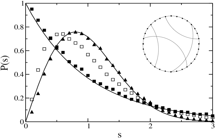
Figure 1: Level spacing statistics for $H$ at $n_{r}=14$, $p=1/32$, for three values of the disorder: $W=0.5$ (triangles), $1.3$ (empty squares) and $3$ (full squares). The solid curves correspond to the Poisson distribution $P(s)=e^{-s}$ and to the Wigner-Dyson distribution $P(s)=(\pi s/2)e^{-\pi s^{2}/4}$. Number of disorder realizations (position of shortcut links and on-site disorder) is $N_{D}=10$. Only the central half of the eigenvalues is taken into account. Inset: a realization of small-world network with $N=32$ and $p=1/8$.

When $p=0$, the system reduces to the one-dimensional Anderson model, for which all states are known to be localized. For small disorder, the localization length $l$ varies as $l\propto 1/W^{2}$ mirlin . The additional presence of shortcut links may induce delocalization. This can be checked through spectral statistics. Indeed, for localized systems, the eigenvalues are distributed according to the Poisson distribution, provided the localization length is smaller than the system size. On the contrary, in the delocalized phase the eigenvalues follow the Wigner-Dyson distribution corresponding to Random Matrix Theory, which generally characterizes quantum chaotic systems and ergodic wavefunctions mirlin . Our numerical diagonalization of $H$ at fixed $p$ shows a transition from Poisson to Wigner distribution as $W$ decreases. A typical example is shown in Fig.1 at $p=1/32$ and $W=3$ (localized phase), $W=1.3$ (intermediate statistics), $W=0.5$ (delocalized phase). This indicates that a delocalization transition takes place in this system.

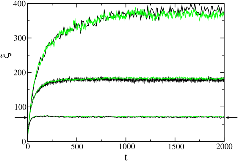
Figure 2: (color online) Evolution of the IPR $\xi$ with time $t$, for $W=0.5$ and $p=1/32$. Initial state is localized on one vertex. Curves correspond (from bottom to top) to $n_{r}=8,10,12$. Each curve is shown as obtained by exact evolution (black lines), with $N_{D}=80$, and by simulation by quantum gates (see text)(green/gray lines) with $N_{D}=100$ and $\Delta t=0.03$. The arrows indicate the IPR at $t=2000$ in the absence of shortcut links $p=0$ (exact evolution and simulation by quantum gates yield the same result, data not shown).

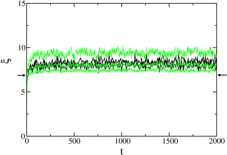
Figure 3: (color online) Same as Fig.2 with $W=3$.

The localization properties of this quantum system can be analyzed more precisely through the Inverse Participation Ratio (IPR), defined by $\xi=\sum_{i}|\Psi_{i}|^{2}/\sum_{i}|\Psi_{i}|^{4}$ for a wavefunction $|\Psi\rangle=\sum_{i}\Psi_{i}|i\rangle$. It gives the number of vertices supporting the wavefunction ($\xi=1$ for a state localized on a single vertex, and $\xi=N$ for a state uniformly spread over $N$ vertices). In Fig.2 and Fig.3, we display the time evolution of the IPR for a wave packet initially localized on one vertex. For $W=0.5$, the saturation value grows with $N$ in the presence of shortcut links, indicating that the wavefunction is no longer localized. On the contrary, for $W=3$, the saturation value remains close to its value in the absence of links and does not change significantly with $N$, implying that the system is still localized. In a more quantitative way, Fig.4 presents the saturation value of the IPR as a function of $n_{r}$ for different values of $p$. The data confirm that at $W=3$ the system remains localized. On the contrary, a clear delocalization is visible in the presence of shortcut links for $W=0.5$. The data are in good agreement with the law $\xi\propto N^{\alpha}$, with $\alpha\approx 0.58$ for $p=1/32$ and $\alpha\approx 0.84$ for $p=1/16$ (the maximal value $\alpha=1$ is obtained at $p=1/2$, data not shown). This shows that the delocalization transition for $p=1/16$ and $p=1/32$ takes place approximately at $W\approx 1$. In the limit of weak disorder $W\ll 1$, the transition is expected to take place at smaller values of $p\propto W^{2}$ como2001 .

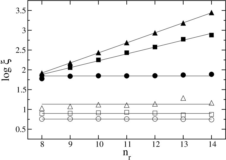
Figure 4: IPR at time $t=2000$ as a function of $n_{r}$ for $W=0.5$ (full symbols) and $W=3$ (empty symbols), for $p=1/16$ (triangles), $p=1/32$ (squares) and $p=0$ (circles), with $20\leq N_{D}\leq 160$. Initial state is localized on one vertex. Straight lines correspond from top to bottom to $\xi=0.78N^{0.84}$, $\xi=3.13N^{0.58}$, $\xi=70.15$, $\xi=13.55$, $\xi=7.91$, $\xi=5.69$, with $N=2^{n_{r}}$. Logarithm is decimal.

This system can be simulated on a quantum computer, using $O((\log N)^{2})$ quantum gates for a network of $N=2^{n_{r}}$ vertices, and $n_{q}=3n_{r}+3$ qubits. We start from an initial wave packet encoded on the quantum registers. For example, the initial one-vertex states used in Figs.2-4 can be constructed efficiently from a state localized in the ground state of the quantum computer by at most $n_{r}$ single-qubit flips. Our quantum algorithm performs the evolution of the wave packet by slicing the propagator $\exp(iHt)$, using the relation $e^{i(H_{0}+H_{1}+H_{2})\Delta t}=e^{iH_{0}\frac{\Delta t}{2}}e^{iH_{1}\frac{\Delta t}{2}}e^{iH_{2}\Delta t}e^{iH_{1}\frac{\Delta t}{2}}e^{iH_{0}\frac{\Delta t}{2}}+O(\Delta t^{3})$ for a short period of time $\Delta t$ (see e.g. Nielsen ; pomerans ). Each unitary operator is then simulated by quantum gates. We use in particular rotations on the $j$-th qubit by an angle $\phi/2$: $R_{j}(\phi)=\exp(i\phi\sigma_{j}^{z}/2)$ ($\sigma^{z}$ being a Pauli matrix); controlled-not operations $\textrm{Cnot}_{i,j}$, that is bit-flip on the $j$-th qubit conditioned by the $i$-th qubit; multi-controlled rotations $C_{i_{1},...,i_{\mu},\eta_{1},...,\eta_{\mu},j}(\theta)$, that is rotations by an angle $\theta$ on the $j$-th qubit if and only if the qubits $i_{k}$ takes the value $\eta_{k}\in\{0,1\}$ for $1\leq k\leq\mu$.

$\bullet$ The transformation $|i\rangle\rightarrow e^{iH_{0}\Delta t}|i\rangle$ consists in multiplying each basis state $|i\rangle$ by a Gaussian random phase $\exp(i\epsilon_{i}\Delta t)$. For some integer $n_{s}$, and $\sigma=W\Delta t\sqrt{\frac{3}{n_{r}+n_{s}}}$, let us choose randomly $n_{r}+n_{s}$ angles $\phi_{k}$, $1\leq k\leq n_{r}$, and $\phi^{\prime}_{k}$, $1\leq k\leq n_{s}$, independent and uniformly distributed in $[-\sigma/2,\sigma/2]$. Each $\epsilon_{i}\Delta t$ is replaced by a random variable $\pm\phi_{1}\pm\phi_{2}\pm\cdots\pm\phi^{\prime}_{s-1}\pm\phi^{\prime}_{s}$, which for large $n_{s}$ tends to a Gaussian random variable of width $W\Delta t$. This can be simulated by applying the operator $\prod_{k=n_{s}}^{1}\textrm{Cnot}_{i_{k},j_{k}}\prod_{k=1}^{n_{s}}\left(R_{j_{k}}(\phi^{\prime}_{k})\textrm{Cnot}_{i_{k},j_{k}}\right)\prod_{k=1}^{n_{r}}R_{k}(\phi_{k})$ for some value of $n_{s}$. The $i_{k}$ and $j_{k}$ are chosen randomly between $0$ and $n_{r}-1$. This step requires $(3n_{s}+n_{r})$ gates.

$\bullet$ To perform the transformation $|i\rangle\rightarrow e^{iH_{1}\Delta t}|i\rangle$, we first apply a quantum Fourier transform (QFT) to turn it into the diagonal transformation $|k\rangle\rightarrow\exp\left(2i\Delta t\cos\frac{2\pi k}{N}\right)|k\rangle$. Following pomerans , we introduce the operator $R_{\gamma}(\bar{\theta})=HS^{1}He^{-i\frac{\gamma}{2}\sigma_{1}^{z}}HS^{-2}He^{-i\frac{\gamma}{2}\sigma_{1}^{z}}HS^{1}$ with $S^{m}=\prod_{j=2}^{n_{r}}C_{1,j}(\pi m/2^{j-1})$. It can be shown that $e^{-i\gamma\cos\theta}=R_{\gamma/2}(\bar{\theta})R_{\gamma/2}(-\bar{\theta})+O(\gamma^{3})$ for small $\gamma$, with $\bar{\theta}=\theta-\pi a_{1}$ if $\theta/2\pi=0.a_{1}a_{2}\ldots a_{n}$. The diagonal operator can thus be approximated by $\exp\left(2i\Delta t\cos\frac{2\pi k}{N}\right)=\left(R_{\gamma/2}(\bar{\theta})R_{\gamma/2}(-\bar{\theta})\right)^{L}+O(L\gamma^{3})$, with $L$ an integer and $\gamma$ a small parameter chosen such that $L\gamma=-2i\Delta t$. We then perform an inverse QFT. The two QFT require $n_{r}(n_{r}+1)$ gates, and the simulation of the diagonal term requires $2L(5+3n_{r})$ gates.

$\bullet$ The transformation $|i\rangle\rightarrow e^{iH_{2}\Delta t}|i\rangle$ acts on the subspace spanned by $|i_{k}\rangle$ and $|j_{k}\rangle$, where $i_{k}$ and $j_{k}$ are linked by a shortcut link, through the $2\times 2$ submatrix $e^{i\Delta t\sigma^{x}}$. Let us first assume that $p$ is of the form $p=1/2^{\rho}$. For $\mu=\rho-1$, the operator $C_{i_{1},...,i_{\mu},\eta_{1},...,\eta_{\mu},j}(\theta)$ acts on the $2^{n_{r}-\mu}$ basis vectors whose qubits $i_{k}$, $1\leq k\leq\mu$, are respectively equal to $\eta_{k}$: it corresponds to the creation of $2^{n_{r}-\mu-1}=2^{n_{r}-\rho}=pN$ links. In order to have less regular shortcut links, we first perform a permutation on the vertices. To do this, we randomly choose $n_{p}$ integers $a_{k}$ and $b_{k}$, for some integer $n_{p}$. It is better to take the $a_{k}$ in $[0.2N,0.8N]$ and odd. Then we define the operators $U_{k}|i\rangle=|(a_{k}i+b_{k})\mod N\rangle$ and the inverse operators $V_{k}|i\rangle=|a_{k}^{-1}(i-b_{k})\mod N\rangle$. A permutation can be simulated by the sequence of gates $P=\prod_{k=1}^{n_{p}}U_{k}\ \textrm{Cnot}_{i_{k},j_{k}}$ where the $i_{k}$ and $j_{k}$ are chosen randomly. Application of the permutation $P$, followed by a multi-controlled rotation $C_{i_{1},...,i_{\mu},\eta_{1},...,\eta_{\mu},j}(\Delta t)$ and $P^{-1}$, gives $e^{iH_{2}\Delta t}$. The $i_{k}$ and $\eta_{k}$ in the controlled rotation are also chosen randomly. In the general case, where $p\neq 1/2^{\rho}$, we expand $pN$ in base 2, such that $pN=\sum 2^{p_{k}}$. Then we replace the multi-controlled gate in the above description by a multi-controlled gate for each $p_{k}$ appearing in the decomposition of $pN$. This gives a sequence of gates $C_{i^{(k)}_{1},...,i^{(k)}_{\mu_{k}},\eta^{(k)}_{1},...,\eta^{(k)}_{\mu_{k}},j^{(k)}}(\Delta t)$, where $\mu_{k}=n_{r}-p_{k}-1$, and the $i^{(k)}_{k^{\prime}}$, $j^{(k)}$ and $\eta^{(k)}_{k^{\prime}}$ are chosen randomly. Each operator $U_{k}$ consists of a multiplication and an addition modulo $N$, which can be performed using $(2n_{r}+3)$ ancilla qubits and $O(n_{r}^{2})$ quantum gates arithm1 . Each multi-controlled gate can be performed by $O(n_{r}^{2})$ Toffoli, Cnot and single qubit gates arithm2 .

In total, the simulation of a network of $N=2^{n_{r}}$ vertices for one unit of time with fixed parameters $\Delta t$, $n_{s}$, $L$ and $n_{p}$ can be done by this method with $O(n_{r}^{2})$ quantum operations and $3n_{r}+3$ qubits. Classically, a similar method can only be implemented in $O(N)$ operations at best. The quantum simulation is therefore exponentially faster. This remains the case even if the parameters $n_{s}$ and $n_{p}$ are allowed to grow linearly with $n_{r}$ to improve accuracy (the cost becomes $O(n_{r}^{3})$ quantum gates).

The algorithm simulates the small-world network efficiently but at the cost of several approximations. In order to check its convergence and accuracy, we implemented it on a (classical) computer. In Figs.2,3, we display the result of this computation for the parameters $\Delta t=0.03$, $n_{s}=30n_{r}$, $L=10$, and $n_{p}=3n_{r}$ alongside the exact evolution, showing that the algorithm is quite accurate for these values, and enables to monitor precisely the delocalization transition with good accuracy. The computation accuracy is not very sensitive to fixed values of $L$ and $\Delta t$: the total size $N$ can be changed by orders of magnitude (factor of $64$ in our case) without modification of these parameters.

To estimate the total complexity of the algorithm, we should take into account the number of quantum measurements and the number of iterations of the map. In order to see the delocalization transition, it is sufficient to estimate the spreading of the wavefunction, which can be done by a constant number of quantum measurements loclength . Still, the initial wave packet should have enough time to spread in order for the localization length to be estimated. For the parameters of Fig.2, we determined the time $\tau$ needed for the IPR to reach half of its maximal value. In the delocalized phase for $p<1/2$, our numerical results give the scaling $\tau\propto N^{\beta}$ with $\beta\approx 0.83$ ($p=1/16$) and $\beta\approx 0.69$ ($p=1/32$) (data not shown). This means that the total cost of the quantum algorithm will scale as $O(N^{\beta})$, compared to $O(N^{\beta+1})$ for the classical one (dropping logarithmic factors). This implies a better than quadratic gain for the quantum computation, but no exponential gain. In contrast, for $1/2<p\leq 2$ we find that $\tau\approx\log N$ (data not shown) footnote2 . In this case, the algorithm may reach exponential efficiency and enable to perform precise studies of this percolation-like transition for very large values of $N$. The exact algorithm complexity depends on the properties of the phase transition near critical $W$ value.

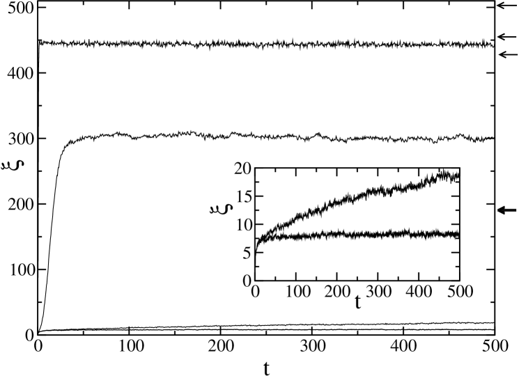
Figure 5: Evolution of the IPR with time in the presence of static errors, for $n_{r}=10$, $W=3$ and $p=1/32$, with $N_{D}=100$ (static errors are the same for all realizations). Initial state is localized on one vertex, $\Delta t=0.03$. From top to bottom: $\epsilon=10^{-4}$, $10^{-5}$, $10^{-6}$, $10^{-7}$ and $0$. The arrows mark $\xi$ at $t=500$ for $W=0.5$ and same other parameters, with from top to bottom $\epsilon=10^{-5}$, $10^{-4}$, $10^{-6}$, $10^{-7}$ and $0$. Inset shows the three lowest curves on a different scale. Data from $\epsilon=10^{-7}$ are indistinguishable from $\epsilon=0$.

These results show that a perfect quantum computer gives a significant gain in the simulation of quantum small-world networks. However, realistic quantum computers are prone to errors and imperfections. It is therefore important to test the resilience of the algorithm to such effects. In Fig.5 we show the result of numerical simulations of the algorithm in presence of errors. The error model chosen corresponds to static imperfections. These errors can exist independently of the coupling with the external world, and have parametrically larger effects than random noise in the gates qchaos . Between each gate the system evolves through the additional Hamiltonian $H_{E}=\sum_{i}\delta_{i}\sigma_{i}^{z}+\sum_{i}J_{i}\sigma_{i}^{x}\sigma_{i+1}^{x}$, where the second sum runs over nearest-neighbor qubit pairs on a circular chain. The $\delta_{i}$ are randomly and uniformly distributed in the interval $[-\delta/2,\delta/2]$. The couplings $J_{i}$ represent the residual static interaction between qubits and are chosen randomly and uniformly in the interval $[-J,J]$. We suppose that each gate in the quantum algorithm is instantaneous and separated by a time $\tau_{g}$ during which $H_{E}$ acts. We take one single rescaled parameter $\varepsilon$ which describes the amplitude of these static errors, with $\varepsilon=\delta\tau_{g}=J\tau_{g}$. In the numerical simulations, to save computational time we took the part of the algorithm which generates the random shortcut links as exact, all other parts being performed with errors. The results displayed in Fig.5 show that with moderate levels of imperfections ($\varepsilon\approx 10^{-7}$) the simulation of the small-world network is very close to the exact computation, in absence of any quantum error correction.

In conclusion, we have shown that quantum disordered small-world networks, which display a delocalization transition, can be simulated more efficiently on quantum computers than on classical ones. The algorithm can be performed accurately on realistic few-qubit quantum computers in presence of moderate error strength.

We thank A. Pomeransky and O. Zhirov for helpful discussions. We thank the IDRIS in Orsay and CalMiP in Toulouse for access to their supercomputers. This work was supported in part by the project EDIQIP of the IST-FET program of the EC.

References

- (1) S. Milgram, Psychol. Today 2, 60 (1967); D. J. Watts and S. H. Strogatz, Nature 393, 440 (1998); M. E. J. Newman, C. Moore and D. J. Watts, Phys. Rev. Lett. 84, 3201 (2000).
- (2) C. P. Zhu and S.-J. Xiong, Phys. Rev. B 62, 14780 (2000).
-
(3)
A. D. Chepelianskii and D. L. Shepelyansky (2001),
www.quantware.ups-tlse.fr/talks-posters/chepelian-
skii2001.pdf - (4) B. J. Kim, H. Hong and M. Y. Choi, Phys. Rev. B 68, 014304 (2003).
- (5) M. A. Nielsen and I. L. Chuang, Quantum computation and quantum information, (Cambridge university press, Cambridge, England, 2000).
- (6) P. W. Shor, in Proceedings of the 35th Annual Symposium on the Foundations of Computer Science, edited by S. Goldwasser (IEEE Computer Society, Los Alamitos, CA, 1994), p. 124.
- (7) L. K. Grover, Phys. Rev. Lett. 79, 325 (1997).
- (8) Shortcuts do not connect nearest-neighbors.
- (9) A. D. Mirlin, Phys. Rep. 326, 259 (2000).
- (10) A. A. Pomeransky and D. L. Shepelyansky, Phys. Rev. A 69, 014302 (2004).
- (11) V. Vedral, A. Barenco and A. Ekert, Phys. Rev. A 54, 147 (1996).
- (12) A. Barenco, C. H. Bennett, R. Cleve, D. P. DiVincenzo, N. Margolus, P. Shor, T. Sleator, J. A. Smolin and H. Weinfurter, Phys. Rev. A 52, 3457 (1995).
- (13) G. Benenti, G. Casati, S. Montangero and D. L. Shepelyansky, Phys. Rev. A 67, 052312 (2003).
- (14) We note that in diffusion a logarithmic law for was also found in another type of quantum small-world network without on-site disorder.
- (15) B. Georgeot and D. L. Shepelyansky, Phys. Rev. E 62, 3504 (2000); ibid. 62, 6366 (2000); K. M. Frahm, R. Fleckinger and D. L. Shepelyansky, Eur. Phys. J. D 29, 139 (2004).