Signatures of chaotic and non-chaotic-like behaviour in a non-linear quantum oscillator through photon detection.

Abstract

The driven non-linear duffing oscillator is a very good, and standard, example of a quantum mechanical system from which classical-like orbits can be recovered from unravellings of the master equation. In order to generate such trajectories in the phase space of this oscillator in this paper we use a the quantum jumps unravelling together with a suitable application of the correspondence principle. We analyse the measured readout by considering the power spectra of photon counts produced by the quantum jumps. Here we show that localisation of the wave packet from the measurement of the oscillator by the photon detector produces a concomitant structure in the power spectra of the measured output. Furthermore, we demonstrate that this spectral analysis can be used to distinguish between different modes of the underlying dynamics of the oscillator.

I Introduction

There is currently an intense interest being shown in the possible application of quantum devices to fields such as computing and information processing Nielsen and Cheung (2000). The goal is to construct machinery which operates manifestly at the quantum level. In any successful development of such technology the role of measurement in quantum systems will be of central, indeed crucial, importance (see for example Shepelyansky (2001)). In order to extend our understanding of this problem we have recently investigated the coupling together of quantum systems that, to a good approximation, appear classical (via the correspondence limit) but whose underlying behaviour is strictly quantum mechanical Everitt et al. (2005). In this work we followed the evolution of two coupled, and identical, quantised Duffing oscillators as our example system. We utilised two unravellings of the master equation to describe this system: quantum state diffusion and quantum jumps which correspond, respectively, to unit-efficiency heterodyne measurement (or ambi-quadrature homodyne detection) and photon detection Wiseman (1996). We demonstrated that the entanglement that exists between the two oscillators depends on the nature of their dynamics. Explicitly, we showed that whilst the dynamics was chaotic-like the entanglement between the oscillators remained high; conversely, if the two oscillators entrained into a periodic orbit the degree of entanglement became very small.

With this background we subsequently became interested in acquiring a detailed understanding of experimental readouts of quantum chaotic-like systems. In this paper we have chosen to explore the subject through the quantum jumps unravelling of the master equation Plenio and Knight (1998); Wiseman (1996); Hegerfeldt (1993). Here, the measured output is easily identified, namely a click or no click in the photon detector. However, this measurement process is rather unique in the fact that it possesses no classical analogue. Indeed, this is the case even when the system under consideration may appear to be evolving along a classical trajectory. Interestingly, despite the fact that the photon detector has no classical analogue, it is the very presence of this as a source of decoherence that is responsible for recovering classical-like orbits in the $\left(\left\langle q\right\rangle,\left\langle p\right\rangle\right)$ phase plane (despite the fact that we measure neither $q$ nor $p$). The subject of recovering such chaotic-like dynamics from unravellings of the master equation has been studied in depth in the literature Percival (1998); Habib et al. (1998); Brun et al. (1997, 1996); Spiller and Ralph (1994) and a detailed discussion is beyond the scope of this paper. However, we note that recently in Peano and Thorwart (2004) resonances have been observed in a model of a non-linear nano-mechanical resonator that is absent in the corresponding classical model. In this present work we have chosen to scale the oscillator so that we recover orbits similar to those generated from a classical analysis.

II Background

In this work we study the output resulting from the measurement of quantum objects where the measurement device generates decoherence effects. In this limit the system exhibits dynamical behaviour in terms of its expectation values very much like those observed in its classical counterpart. In this work we investigate the region of parameter space under which the classical system exhibits chaotic motion. Of the many models that could be used we have chosen the Quantum Jumps approach Plenio and Knight (1998); Wiseman (1996); Hegerfeldt (1993). We note that this is only one of several possible unravellings of the master equation that correspond to the continuous measurement of the quantum object considered. Our motivation for using this approach is that the recorded output of the measurement is completely transparent i.e. the photon counter either registers a photon or it does not.

In the quantum jumps unravelling of the master equation the evolution of the (pure) state vector $\left|\psi\right\rangle$ for an open quantum system is given by the stochastic Itô increment equation

$$\left|d\psi\right\rangle=-\frac{i}{\hbar}H\left|\psi\right\rangle dt-\frac{1}{2}\sum_{j}\left[L_{j}^{\dagger}L_{j}-\left\langle L_{j}^{\dagger}L_{j}\right\rangle\right]\left|\psi\right\rangle dt+\sum_{j}\left[\frac{L_{j}}{\sqrt{\left\langle L_{j}^{\dagger}L_{j}\right\rangle}}-1\right]\left|\psi\right\rangle dN_{j}$$ (1)

where $H$ is the Hamiltonian, $L_{i}$ are the Linblad operators that represent coupling to the environmental degrees of freedom, $dt$ is the time increment, and $dN_{j}$ is a Poissonian noise process such that $dN_{j}dN_{k}=\delta_{jk}dN_{j}$, $dN_{j}dt=0$ and $\overline{dN_{j}}=\left\langle L_{j}^{{\dagger}}L_{j}\right\rangle dt$. These latter conditions imply that jumps occur randomly at a rate that is determined by $\left\langle L_{j}^{{\dagger}}L_{j}\right\rangle$. We will find that this is very important when explaining the results presented later in this paper. For an excellent discussion of quantum trajectories interpreted as a a realistic model of a system that is being continuously monitored see Wiseman (1996). For an interesting and more general discussion on the emergence of classical-like behaviour from quantum systems see D. et al. (1996); Joos et al. (2003).

The Hamiltonian for our, standard, example system of the Duffing oscillator is given by

$$H=\frac{1}{2}p^{2}+\frac{\beta^{2}}{4}q^{4}-\frac{1}{2}q^{2}+\frac{g}{\beta}\cos\left(t\right)q+\frac{\Gamma}{2}\left(qp+pq\right)$$ (2)

where $q$ and $p$ are the canonically conjugate position and momentum operators for the oscillator. In this example we have only one Linblad operator which is $L=\sqrt{2\Gamma}a$, where $a$ is the oscillator annihilation (lowering) operator, $g$ is the drive amplitude and $\Gamma=0.125$ quantifies the damping.

In order to apply the correspondence principal to this system, and recover classical-like dynamics, we have introduced in Eq. (2) the parameter $\beta$. For this Hamiltonian it has two interpretations that are mathematically equivalent. Firstly, it can be considered to scale $\hbar$ itself, or, alternatively we can simply view $\beta$ as scaling the Hamiltonian, leaving $\hbar$ fixed, so that the relative motion of the expectation values of the observables becomes large compared with the minimum area $\left(\hbar/2\right)$ in the phase space. In either case, the system behaves more classically as $\beta$ tends to zero from its maximum value of one. In this work we have chosen to set $\beta=0.1$.

III Results

(a) Classical Duffing oscillator.

(b) Quantum Duffing oscillator.

Figure 1: Power spectrum of the position, $x$ for the classical Duffing oscillator and $\left\langle q\right\rangle$ for the quantum Duffing oscillator $\beta=0.1$. The frequency is normalised to the drive frequency of the oscillator.

Let us now consider the specific example of a Duffing oscillator with a drive amplitude $g=0.3$. This parameter, together with all the those already specified, form the classic example used to demonstrate that chaotic-like behaviour can be recovered for open quantum systems by using unravellings of the master equation Percival (1998); Brun et al. (1997, 1996); Everitt et al. (2005). In Fig. 1 we compare the power spectra of the classical position coordinate with that of $\left\langle q\right\rangle$. Here noise has been added to the classical system so as to mimic the level of quantum noise that is present in the stochastic elements of our chosen unravelling of the master equation and we have solved for a realisation of the Lagivan equation. As can be seen, for this value of $\beta$ there is a very good match between these two results. Moreover, both display power spectra that are typical for oscillators in chaotic orbits.

However, it is not position that is the measured output in this model, but the quantum jumps recorded, as a function $\mathcal{N}(t)$ of time in the photon detector. As stated above, these jumps occur randomly at a rate that is determined by $\left\langle L_{j}^{{\dagger}}L_{j}\right\rangle$ which, for this example, is $2\Gamma\left\langle n\right\rangle$. Hence, the probability of making a jump is proportional to the number of photons in the state of the system at any one time.

(a) Power spectrum of $\left\langle q\right\rangle$.

(b) Power spectrum of $\mathcal{N}(t)$.

Figure 2: Power spectrum of the position $\left\langle q\right\rangle$ and photons counted $\mathcal{N}(t)$ for the quantum simple harmonic oscillator in a steady state. Here the frequency is normalised to the drive frequency of the oscillator.

We now consider a special case that occurs frequently in the classical limit, namely where $\left|\psi\right\rangle$ localises approximately to a coherent (Gaussian) state. It is apparent that for such a state the chance of observing a jump is proportional to the square of the distance in $\left(\left\langle q\right\rangle,\left\langle p\right\rangle\right)$ of the state from the origin. In order to illustrate the implications of this, let us consider a driven simple harmonic oscillator. The Hamiltonian is

$$H_{s}=\frac{1}{2}p^{2}+\frac{1}{2}q^{2}+\frac{g}{\beta}\cos\left(t\right)q$$

and we note that in this special case the only effect of $\beta=0.1$ is to scale the amplitude of the drive (again we set $g=0.3$). We now solve Eq. (1) using this Hamiltonian and allow the system to settle into a steady state. Then, as the phase portrait for this system simply describes a circle centred about $(0,0)$ we would expect the power spectra of photons counted to be the same as those for white noise. Indeed, this is clearly seen in Fig. 2 where we show the power spectrum for both (a) the position operator and (b) the measured quantum jumps.

Figure 3: Power spectrum of the measured quantum jumps $\mathcal{N}(t)$ for the Duffing oscillator of Fig. 1(b).

For more complicated orbits, such as those exhibited by the Duffing oscillator, we would expect to see some evidence of the underlying dynamical behaviour. Hence, localisation of $\left|\psi\right\rangle$ from the measurement of the Duffing oscillator through the photon detector forms a concomitant structure in the power spectrum of the measured output. In Fig. 3 we show, for comparison with 1(b), such a power spectrum.

As we can see from Fig. 3 the power spectrum for this chaotic mode of operation reveals some structure. However, it is not clear from this picture alone how we might relate this result to that shown in Fig. 1(b). It is therefore reasonable to ask if this result does indeed tell us anything about the underlying dynamics of the oscillator. We have addressed this point by computing the power spectrum of both $\left\langle q\right\rangle$ and $\mathcal{N}(t)$ for drive amplitudes in the range $0<g\leq 3$, the results of which are presented in Fig. 4.

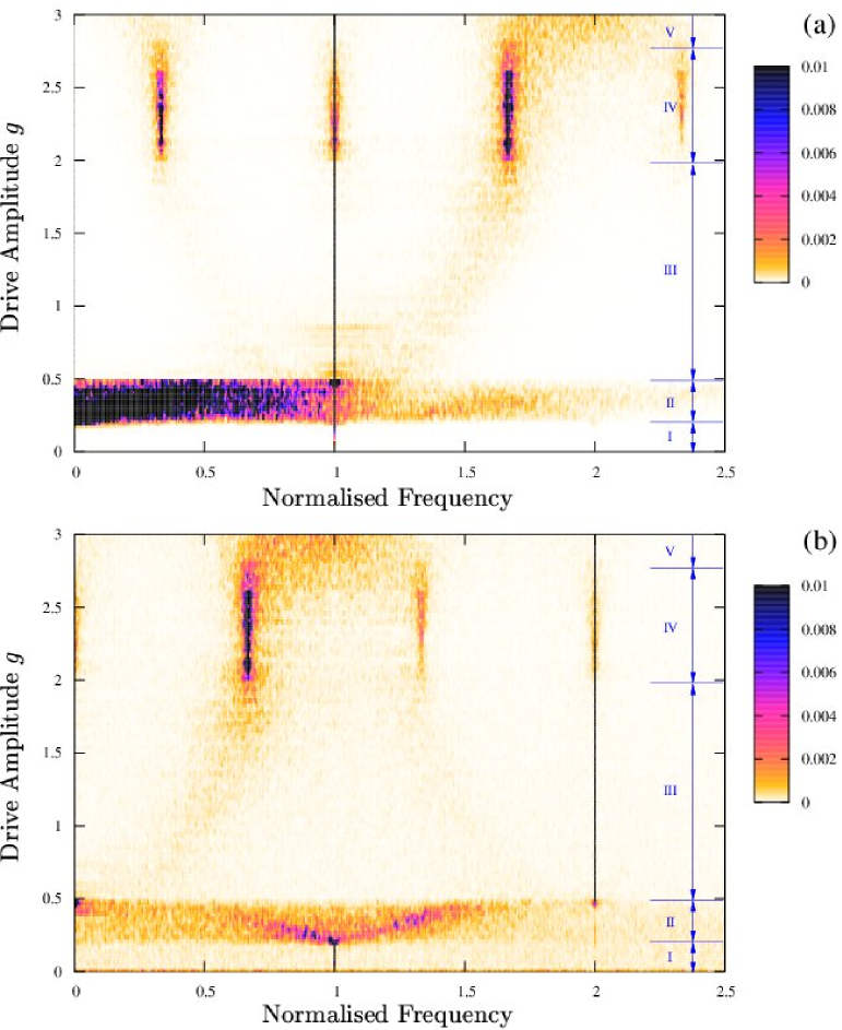
Figure 4: (color online) Power spectrum of the (a) $\left\langle q\right\rangle$ and (b) measured quantum jumps as a function of drive amplitude.

Although the functional form of these power spectra obviously differ, they do clearly exhibit changes in behaviour that are coincident in the drive amplitudes of both figures. These are identified as intervals in $g$ labelled I, II, …in Fig. 4.

(a) Power spectrum of $\left\langle q\right\rangle$, $g=0.1$.

(b) Power spectrum of $\mathcal{N}(t)$, $g=0.1$.

(c) Power spectrum of $\left\langle q\right\rangle$, $g=0.3$.

(d) Power spectrum of $\mathcal{N}(t)$, $g=0.3$.

(e) Power spectrum of $\left\langle q\right\rangle$, $g=1.25$.

(f) Power spectrum of $\mathcal{N}(t)$, $g=1.25$.

(g) Power spectrum of $\left\langle q\right\rangle$, $g=2.5$.

(h) Power spectrum of $\mathcal{N}(t)$, $g=2.5$.

Figure 5: Example power spectra for four different drive amplitudes corresponding to the regions I to IV as marked in the power spectrum of Fig. 4.

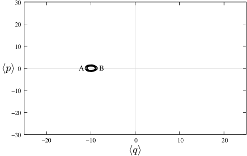
(a) Region I - the drive $g=0.1$ (periodic stable orbit).

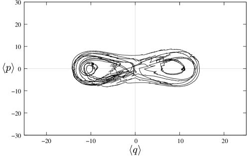
(b) Region II - the drive $g=0.3$ (chaotic-like trajectory).

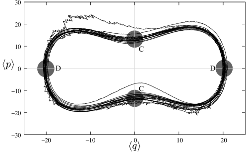
(c) Region III - the drive $g=1.25$ (periodic stable orbit).

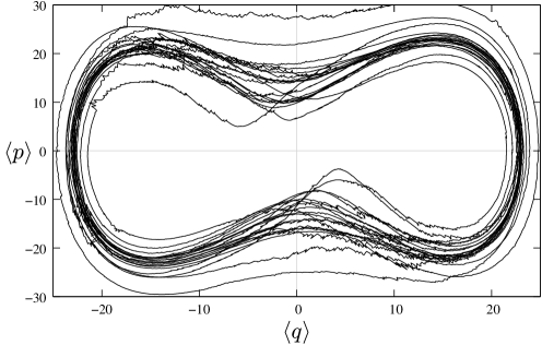
(d) Region IV - the drive $g=2.5$ (quasi-periodic orbit).

Figure 6: Example phase portraits for four different drive amplitudes corresponding to the regions I to IV as marked in the power spectrum of Fig. 4.

To help clarify Fig. 4 we provide in Fig. 5 explicit power spectra of both $\left\langle q\right\rangle$ and the quantum jumps $\mathcal{N}(t)$ for regions I-IV. As expected for region I in Figs. 5(a) and 5(b) we see a strong resonance at the frequency of the drive. The broadband behaviour characteristic of the chaotic phenomena associated with region II is evident in Fig. 5(c) and a concomitant, although different, structure in the power spectrum of the detected photons. In region III of Fig. 4 we again return to a periodic orbit. In Fig. 5(e), the power spectra for $\left\langle q\right\rangle$ exhibits a peak at the drive frequency, however, the power spectra of $\mathcal{N}(t)$ peaks at twice this frequency. The lack of coincidence between these two figures will be explained fully in the following text. Finally in Figs. 5(g) and 5(h) we see power the power spectrum of the quasi periodic dynamics of region IV, again the discrepancy between these two figures is discussed below.

The mechanism through which the detection of photons can yield significant information about the underlying dynamics of the system can be understood by looking at the phase portraits of $\left\langle q\right\rangle$ and $\left\langle p\right\rangle$ associated with the regions I–IV of Fig. 4 for those values of drive used in Fig. 5, these are shown in Fig. 6.

For region I there is a strictly periodic response on both power spectra at the drive frequency of the oscillator. It can be seen from Fig. 6(a) that, because of the distance from the origin, the chance of there being a photon counted at point A is more likely than at point B. As this occurs at the same frequency as the oscillations of $\left\langle q\right\rangle$, we have direct agreement in the position of the resonance in each of the different spectra.

In region II, and as is clear from Fig. 6(b), the system is following a chaotic-like trajectory. Although the power spectra differ drastically in their structure, they do both exhibit broad band behaviour that is characteristic of chaotic orbits.

As the drive amplitude is increased further, region III in Fig. 4 is accessed as the behaviour observed in region II ceases. For this range of drive amplitudes the solution is again a stable periodic orbit as displayed in Fig. 6(c). However, this time, whilst the power spectrum of $\left\langle q\right\rangle$ exhibits a resonance at the drive frequency, that of $\mathcal{N}(t)$ appears at double this frequency. The explanation for this is simply that the probability of detecting a photon when the orbit is in a region of phase space near the origin, such as those marked C in Fig. 6(c), is less that at those further away as in the region of D. This variation in probability occurs twice a period and therefore produces a resonance at double the drive frequency. An immediate corollary is that, by detecting a resonance at either of these different frequencies in the power spectra of $\mathcal{N}(t)$, we can determine whether the oscillator is in region I or III of Fig. 4. From our analysis in Everitt et al. (2005) it may, in some circumstances, be advantageous to place the system in a chaotic orbit. It is possible that this sort of analysis could be used to increase or decrease drive amplitude as part of a feedback and control element for quantum machinery.

Finally, the power spectrum of $\left\langle q\right\rangle$ in region IV of Fig. 4 (a) is characteristic of quasi-periodic behaviour. Using a similar argument to the one above, we can transfer these features onto the spectrum of $\mathcal{N}(t)$. If we compare this result with the, albeit noisy, phase portrait of Fig. 6(d) there is clear evidence of quasi-periodic behaviour.

We have demonstrated, using the Duffing oscillator as our example system, that the different features exhibited in the power spectrum of the photon count can be associated with concomitant features in the power spectrum of the position operator (and vice versa). We note that for any given experimental system where there is a direct correspondence between the power spectrum of $\mathcal{N}$ and $\left\langle x\right\rangle$ that the power spectrum of $\mathcal{N}$ provides us with the same amount of information about the underlying dynamics (e.g. chaotic, quasi-periodic etc.) as the power spectrum of $\left\langle x\right\rangle$. We would like to emphasise that if this direct correspondence did not exist then we would not necessarily be able to make such an assertion. For example, this situation might occur for a system in which there was a high degree of symmetry in the $\left\langle x\right\rangle-\left\langle p\right\rangle$ phase portrait. However, such a detailed study is beyond the scope of this paper.

IV Conclusion

In this work we have shown that, via analysis of the power spectra of the photons detected in a quantum jumps model of a Duffing oscillator, we can obtain signatures of the underlying dynamics of the oscillator. Again, we note that the decoherence associated with actually measuring these jumps is that which, through localisation of the state vector, enables these classical-like orbits to become manifest. We have also demonstrated that the power spectra of the counted photons can be used to distinguish between different modes of operation of the oscillator. Hence, this or some form of time-frequency analysis, could be used in the feedback and control of open quantum systems, a topic likely to be of interest in some of the emerging quantum technologies.