Entanglement of Two Impurities through Electron Scattering

Abstract

We study how two magnetic impurities embedded in a solid can be entangled by an injected electron scattering between them and by subsequent measurement of the electron’s state. We start by investigating an ideal case where only the electronic spin interacts successively through the same unitary operation with the spins of the two impurities. In this case, high (but not maximal) entanglement can be generated with a significant success probability. We then consider a more realistic description which includes both the forward and back scattering amplitudes. In this scenario, we obtain the entanglement between the impurities as a function of the interaction strength of the electron-impurity coupling. We find that our scheme allows us to entangle the impurities maximally with a significant probability.

Recently there has been an increasing interest on the generation of entanglement among spins in mesoscopic solid state structures stationary ; kane ; yamamoto ; mobile ; antonio ; bose-home ; saraga ; beenakker1 ; beenakker . While there are several schemes for entangling adjacent stationary spins through a direct quantum gate between them stationary ; kane ; yamamoto , there is an unfortunate dearth of schemes for entangling well separated stationary spins in such structures. An overwhelming majority of the proposed schemes in which one obtains a reasonable separation between the entangled spins are for mobile entities mobile ; antonio ; bose-home ; saraga ; beenakker1 ; beenakker . Entangling well separated stationary spins is practically important because they can be constituents (qubits) of distinct quantum computers. Establishing entanglement between them is equivalent to linking these computers. Even if they themselves are not parts of quantum computers, they can each have a switchable interaction with static spin qubits of well separated quantum computers. In absence of a method of entangling well separated stationary spins, one has to design a scheme to either stop mobile spins after they have traversed a distance, or find a scheme for mapping their state on to stationary spins. In addition to the above pragmatic application, such entangled stationary spins will also enable one to test Bell’s inequalities with massive particles, which is yet to be done for a significant separation trap-bell . Of course, mobile entangled electrons can also enable such tests with the individual spins being measured by spin filters or spin selective detectors kawabata ; fazio . There are also proposals for Bell’s inequality measurements using the orbital or path, as opposed to the spin, degree of freedom of mobile entities ionicou ; beenakker ; buttiker . However, quite a few of the proposals for the measurement of a single spin, such as those based on scanning tunnelling microscopy or magnetic resonant force microscopy are specific to stationary spins single-spin-meas . These spin measurement methods could be used in a Bell inequality experiment if one were able to entangle well separated stationary spins.

With the above motivations is mind, in this article we propose a scheme to entangle two magnetic impurities (stationary spins $1/2$) embedded in a solid state system. The main idea is to use a ballistic electron as an agent which scatters off the two impurities in succession and entangles them. Being a scattering based scheme, it requires no control over the ability to switch interactions on and off between entities in a solid, as is required by many existing entangling proposals mobile . Moreover, even in comparison to other reduced control proposals, such as those based on scattering or two particle interference antonio ; bose-home , our current scheme has the simplicity that it involves only one mobile entity, namely the ballistic electron, and does away with the difficulty of having to make two electrons coincide at the same place at the same time.

We comment first on the geometry of the system. Since entanglement generation depends on a conduction electron interacting with both impurities, it is most convenient to make the system’s cross section as small as possible. In this spirit, and for the sake of simplicity, we consider a one-dimensional metallic atomic chain (of non-magnetic atoms), with two embedded (substitutional) spin-$1/2$ magnetic impurities. This is shown in Fig. 1.

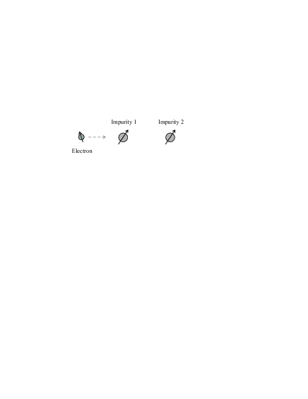
Figure 1: Setup for our scheme to entangle two magnetic impurities of spin $1/2$ in a solid through electron scattering. We consider the simple case of a one-dimensional metallic atomic chain (of non-magnetic atoms) where the two impurities are embedded. The electron flies along the chain and its spin interacts with the spins of the impurities, scattering the electron off and entangling the two impurities.

We know that in an ideal case, where a mediating agent is allowed to interact with two systems through distinct unitary operations, it can then perfectly entangle them. The first of these unitaries perfectly entangles the first system with the agent, and then the second operation swaps the state of the agent with that of the second system. This technique has, for example, been used in proposals for entangling the state of cavities using flying atoms haroche . The different unitaries are implemented by different interaction times or strengths between the agent and each of the systems. Such a technique obviously requires either a great control over the motion of the agent, or the non-trivial engineering of different interaction strengths of the agent with the systems. Under these circumstances, it becomes interesting to investigate the reduced control situation where an agent interacts with both systems through the same unitary operation. How well can the systems be entangled under these circumstances? In the context of quantum optics, one can think of this as an atom having the same flight time and interaction strength with two cavities through which it flies in succession. An analog of this scenario in solid state systems would be to have an electron flying past two identical impurities with the same velocity, interacting magnetically with them successively without any scattering. We first consider this simplified case, just in order to investigate how much entanglement can be established between two impurities, even when the electron interacts with them through the same unitary. We find that a significant entanglement can be established with a significant probability as long as we can make an appropriate measurement of the state of the electron after its successive interaction with the two impurities. This case may not be realistic from the solid state scattering scenario, but it is an interesting precursor to the case when spatial scattering is involved. Moreover, it can be realized in a quantum optics setting where the electronic spin states are replaced by the atomic internal states and impurity states are replaced by zero and one photon states in the cavities. We then proceed to the realistic case of the electron being spatially scattered by the interaction with the impurities. Interestingly, in this case, we find that the electron can entangle the two impurities near perfectly (conditional on a favorable outcome of a measurement of the electron’s spin). Moreover, the probability of this favorable outcome is significant (above 40 percent), which means that on average one should be able to perfectly entangle the impurities with three attempts.

We begin by considering the ideal scenario where the electron’s spin interacts in succession with each of the impurity spins through the Hamiltonian

$$H=J\overrightarrow{S}.\overrightarrow{\sigma},$$ (1)

where $\overrightarrow{\sigma}$ refers to the Pauli operators of the electronic spin, $\overrightarrow{S}$ refers to Pauli operators for the impurity spins and $J$ is the coupling constant between the spins. We now assume that the electron interacts with the two impurities in succession for equal intervals of time, so that with both impurities the same unitary operation is implemented. The joint unitary operation between the electron and impurity $\iota$ (with $\iota=1,2$) as a function of the interaction time $t$ is given by (expressing the unitary operation in terms of its eigenstates):

$$U_{e\iota}(t) = e^{-itH}$$ (2)

$$= e^{i3Jt}|\Psi^{-}\rangle\langle\Psi^{-}|_{e\iota}$$

$$+ e^{-iJt}\left(|\!\uparrow\uparrow\rangle\langle\uparrow\uparrow\!|+|\!\downarrow\downarrow\rangle\langle\downarrow\downarrow\!|\right)_{e\iota}$$

$$+ e^{-iJt}|\Psi^{+}\rangle\langle\Psi^{+}|_{e\iota},$$

where

$$|\Psi^{\pm}\rangle_{e\iota}=\frac{1}{\sqrt{2}}\left(|\!\uparrow\downarrow\rangle_{e\iota}\pm|\!\downarrow\uparrow\rangle_{e\iota}\right).$$ (3)

Let us consider the following initial state where the impurity spins are aligned, and the electron’s spin is anti-aligned with them

$$|\psi_{0}\rangle=|\!\uparrow\rangle_{e}|\!\downarrow\rangle_{1}|\!\downarrow\rangle_{2}.$$ (4)

The final state is then given by

$$|\psi_{f}\rangle=U_{e2}(t)U_{e1}(t)|\psi_{0}\rangle=$$ (5)

$$\frac{e^{-i2Jt}}{2}\left(\alpha|\!\uparrow\rangle_{e}|\!\downarrow\rangle_{1}|\!\downarrow\rangle_{2}+\beta|\!\downarrow\rangle_{e}|\!\uparrow\rangle_{1}|\!\downarrow\rangle_{2}+\gamma|\!\downarrow\rangle_{e}|\!\downarrow\rangle_{1}|\!\uparrow\rangle_{2}\right),$$

where $\alpha=(1+e^{i4Jt})^{2}/2$, $\beta=1-e^{i4Jt}$ and $\gamma=(1-e^{i8Jt})/2$. Each interaction either leaves the direction of the spins unchanged, either flips the interacting pair. Note that if we now measure the spin of the electron and observe the state $|\!\!\downarrow\rangle_{e}$, the impurities will be left in the entangled state $\beta|\!\!\uparrow\rangle_{1}|\!\!\downarrow\rangle_{2}+\gamma|\!\!\downarrow\rangle_{1}|\!\!\uparrow\rangle_{2}$. In Fig. 2 we present the probability of this outcome (dashed line), as well as the resulting amount of entanglement quantified by the entanglement of formation entform (solid line) between the two impurities, both as a function of $Jt$, the product of the interaction strength and the interaction time. We study the probability and the entanglement as a function of $Jt$ in the interval $[0,\pi/2]$ as they are periodic functions, and observe that in this ideal model maximal entanglement is generated only with zero probability. This, however, does not rule out the possibility of obtaining a high amount of entanglement with a significant probability: for example, an entanglement of $0.99$ with a probability of $0.41$, or an entanglement of $0.84$ with a probability of $0.86$ as seen from Fig. 2.

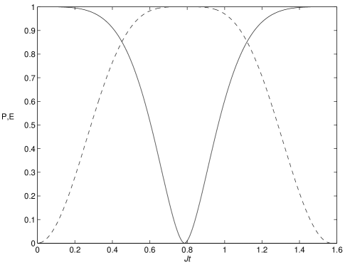
Figure 2: Ideal case — Plots of the probability of success $P$ (dashed line) of detecting the transmitted electron in the spin down state, and the entanglement $E$ (solid line) obtained between the impurity spins in that case, as a function of $Jt$, for the ideal scenario where the electron successively interacts with the two impurities through the same unitary operation. It is clear that one can obtain a high amount of entanglement with a significant probability: for example, an entanglement of $0.99$ with a probability of $0.41$, or an entanglement of $0.84$ with a probability of $0.86$.

Let us now move to a more realistic scattering scenario. Magnetic impurities embedded in a conduction electron sea are traditionally modelled by a s-d Hamiltonian hewson . In this model the magnetic impurities are localized spins interacting with the conduction electrons via an exchange term. The full hamiltonian of a system with one impurity reads

$$H=\sum_{k,\sigma}\varepsilon_{k}a^{\dagger}_{k\sigma}a_{k\sigma}+\sum_{kk^{\prime}}J_{kk^{\prime}}\vec{S}.\vec{s}_{kk^{\prime}}\,,$$ (6)

where $\vec{S}$ is the impurity spin operator, $a^{\dagger}_{k\sigma}$ creates an electron with wavevector $k$ and spin $\sigma$ and

$$\vec{s}_{kk^{\prime}}=\hat{a}^{\dagger}\vec{\sigma}\hat{a}\,,$$ (7)

with $\hat{a}=\left(\begin{array}[]{c}a_{k\uparrow}\\ a_{k\downarrow}\end{array}\right).$ The s-d Hamiltonian is actually derived from the more fundamental Anderson Hamiltonian through the Schrieffer-Wolff transformation. As a consequence, the interaction strength $J$ is related to the strength of the Coulomb interaction between electrons and the hybridization of narrow and conduction bands hewson . In our calculation we will adopt the usual assumption that $J$ is independent of $k,k^{\prime}$.

We want to find out how much entanglement may be generated by a conduction electron that is injected in the system and interacts with both magnetic impurities. One may determine the system’s final state by calculating the scattering matrix associated with each impurity and combining them together. The result is a sequence of (infinitely many) scattering processes, in which the output of a scattering event is the input of the subsequent one. The result of each individual scattering process is determined by use of Fermi’s golden rule. The relevant $T$-matrix is calculated to first order in the interaction.

If we consider that the conduction electron is being injected under low bias, its energy and wavevector will be the Fermi energy and Fermi wavevector of the system, respectively. We thus assume a initial state of the form

$$|\psi_{in}\rangle=|k_{F},\uparrow\rangle_{e}|\!\downarrow\downarrow\rangle_{12}\,,$$ (8)

that represents a conduction electron with positive Fermi wavevector $k_{F}$ and spin $\uparrow$ along the quantization axis ($z$, for instance) propagating towards the two impurities, whose spins are both $\downarrow$ along the $z$-axis.

As a result of the multiple scatterings of the conduction electron by the two impurities, a final state is generated which is a superposition of states in which the conduction electron has been reflected ($r$) or transmitted ($t$),

$$|\psi_{out}\rangle=|\psi_{out}^{r}\rangle+|\psi_{out}^{t}\rangle\,,$$ (9)

and the transmitted component reads

$$|\psi_{out}^{t}\rangle=$$ (10)

$$A|k_{F},\uparrow\rangle_{e}|\!\downarrow\downarrow\rangle_{12}+B|k_{F},\downarrow\rangle_{e}|\!\uparrow\downarrow\rangle_{12}+C|k_{F},\downarrow\rangle_{e}|\!\downarrow\uparrow\rangle_{12}\,.$$

The coefficients $A$, $B$ and $C$ may be expressed as an infinite sum of powers of the product $J\rho(\varepsilon_{F})$, which, according to our estimates antonio , is of the order of unit. We verified numerically that the series converges rapidly for $J\rho(\varepsilon_{F})\in[0,2]$. Below we present the series up to sixth order in $J\rho(\varepsilon_{F})$ (corresponding to three iterations of the scattering matrix),

$$A^{(3)}=\frac{1}{N}(t^{2}+t^{2}\lambda^{2}-8t\lambda^{3}+16\lambda^{6}-7t^{2}\lambda^{4})$$

$$B^{(3)}=\frac{1}{N}(-2\lambda t+2t\lambda^{3}-2t^{2}\lambda^{2}+6t\lambda^{5}+8t^{2}\lambda^{4})$$

$$C^{(3)}=\frac{1}{N}(-2\lambda t+8\lambda^{4}-2t\lambda^{3}+2t^{2}\lambda^{2}+6t\lambda^{5})\,,$$ (11)

where $\lambda=\pi iJ\rho(\varepsilon_{F})/2$, $t=1-\lambda$ and $\frac{1}{N}=\sqrt{|A^{(3)}|^{2}+|B^{(3)}|^{2}+|C^{(3)}|^{2}}$.

We now proceed to calculate the amount of entanglement (as quantified by the entanglement of formation) generated conditional on an electron being transmitted, which is the entanglement contained in the state $|\psi_{out}^{t}\rangle$. Notice that if the transmitted electron has spin up the final state has zero entanglement. Thus we will only evaluate the entanglement of the state in which the transmitted electron has spin down. Fig. 3 shows the entanglement in this state (solid line) and the probability $P$ of observing a transmitted electron with spin up (dashed line). One may notice that there is some entanglement for most of the range $0<J\rho(\varepsilon_{F})<2$, and the probability $P$ is also considerable. Moreover, there are values of $J\rho(\varepsilon_{F})$ for which the entanglement is maximum, and $P$ is significant ($0.41$). It is somewhat interesting to note that although in the ideal case one cannot prepare the impurities in a maximally entangled state with a non-vanishing probability, one can do so in the realistic case.

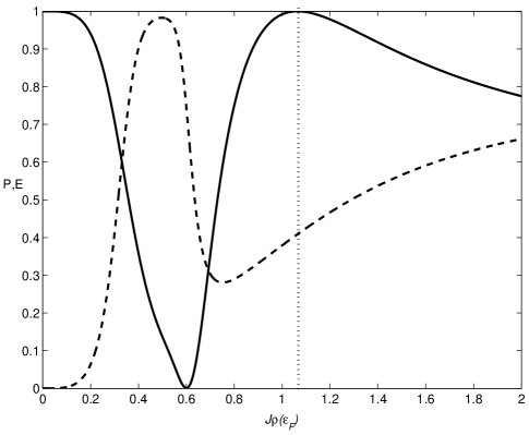
Figure 3: Realistic case — Plots of the probability $P$ (dashed line) of detecting the transmitted electron in the spin down state, and the amount of entanglement $E$ (solid line) obtained between the impurity spins in that case, as a function of the interaction strength $J\rho(\epsilon_{F})$, for the realistic scenario of the electron successively scattering off the two impurities. It is clear that at certain values of $J\rho(\epsilon_{F})$, as shown by the dotted vertical line, the impurities can be projected on to a maximally entangled state with a significant ($0.41$) probability of success.

In this article, we have presented a scheme for entangling two magnetic impurities in a solid through the scattering of a single ballistic electron. While much work has been done on entangling spins in mesoscopic solid state systems, this is the first proposal for entangling distant stationary spins without the aid of an array of intervening spins. An immediate consequence will be in testing Bell’s inequalities with well separated stationary spins in a solid (of course, we still have to measure the spin of a mobile electron, but not when testing Bell’s inequalities). A more far reaching and more significant consequence will be in interfacing distant spin quantum computers. Our work shows that maximal entanglement can be obtained between the distant stationary spins with a significant probability. The scheme should be implementable using the same systems as those used to study Kondo physics kondo . In the future, it will be interesting to explore the types of multi-particle entangled states that can be obtained by the scattering of a single electron from a series of such impurities.

- (1) D. Loss and D. P. DiVincenzo, Phys. Rev. A 57 , 120 (1998); G. Burkard, D. Loss and D. P. DiVincenzo, Phys. Rev. B 59 , 2070 (1999); A. Imamoglu et. al., Phys. Rev. Lett. 83 , 4204 (1999); X. Hu, R. de Sousa and S. Das Sarma Phys. Rev. Lett. 86, 918 (2001); D. Mozyrsky, V. Privman and M. L. Glasser, Phys. Rev. Lett. 86, 5112 (2001); R. Vrijen et. al., Phys. Rev. A 62, 012306 (2000).
- (2) B. E. Kane, Nature 393, 133 (1998).
- (3) W. D. Oliver, F. Yamaguchi and Y. Yamamoto, Phys. Rev. Lett. 88, 037901 (2002).
- (4) D. Loss and E.V. Sukhorukov, Phys. Rev. Lett. 84, 1035 (2000); P. Recher, E. V. Sukhorukov and D. Loss, Phys. Rev. B 63, 165314 (2001); G.B. Lesovik, T. Martin, G. Blatter, Eur. Phys. J. B 24, 287 (2001); P. Samuelsson, E.V. Sukhorukov and M. Büttiker, Phys. Rev. Lett. 91, 157002 (2003); C. Bena, S. Vishveshwara, L. Balents, M.P.A. Fisher, Phys. Rev. Lett. 89, 037901 (2002).
- (5) A. T. Costa Jr. and S. Bose, Phys. Rev. Lett. 87, 277901 (2001).
- (6) S. Bose and D. Home, Phys. Rev. Lett. 88, 050401 (2002).
- (7) D. S. Saraga and D. Loss, Phys. Rev. Lett. 90, 166803 (2003).
- (8) A. V. Lebedev, G. Blatter, C. W. J. Beenakker, G. B. Lesovik, Phys. Rev. B 69, 235312 (2004).
- (9) C. W. J. Beenakker, C. Emary, M. Kindermann and J. L. van Velsen, Phys. Rev. Lett. 91, 147901 (2003).
- (10) M.A. Rowe, D. Kielpinski, V. Meyer, C.A. Sackett,W.M. Itano, C. Monroe, and D.J. Wineland, Nature 409, 791 (2001).
- (11) S. Kawabata, J. Phys. Soc. Jpn. 70, 1210 (2001).
- (12) L. Faoro, F. Taddei, R. Fazio, Phys. Rev. B 69, 125326 (2004).
- (13) R. Ionicioiu, P. Zanardi and F. Rossi, Phys. Rev. A 63, 050101(R) (2001).
- (14) P. Samuelsson, E.V. Sukhorukov, M. Büttiker, Phys. Rev. Lett. 92, 026805 (2004).
- (15) G. P. Berman et. al. quant-ph/0108025; Y. Manassen, I. Mukhopadhyay and N. R. Rao, Phys. Rev. B. 61, 16223 (2000).
- (16) L. Davidovich, N. Zagury, M. Brune, J.M. Raimond, and S. Haroche Phys. Rev. A 50, R895-R898 (1994).
- (17) W. K. Wootters, Phys. Rev. Lett. 80, 2245 (1998).
- (18) A.C. Hewson, The Kondo Problem to Heavy Fermions, Cambridge Studies in Magnetism vol. 2, Cambridge University Press, Cambridge 1997.
- (19) S. Sasaki et al., Nature 405, 764 (2000); J. Nygard, D. H. Cobden and P. E. Lindelof, Nature 408, 342 (2000); V. Madhavan et. al. Science 280, 567 (1998); T.W. Odom, J.L. Huang, C.L. Cheung, and C.M. Lieber, Science 290, 1549 (2000).