Quantum logic via optimal control in holographic dipole traps

Abstract

We propose a scheme for quantum logic with neutral atoms stored in an array of holographic dipole traps where the positions of the atoms can be rearranged by using holographic optical tweezers. In particular, this allows for the transport of two atoms to the same well where an external control field is used to perform gate operations via the molecular interaction between the atoms. We show that optimal control techniques allow for the fast implementation of the gates with high fidelity.

1 Introduction

In the search for a suitable system for quantum information processing, certain requirements have to be met [1], such as scalability of the physical system, the capability of initializing and reading out the qubits, and the possibility of having a set of universal logic gates. Neutral atoms are one of the most promising candidates for storing and processing quantum information. A qubit can be encoded in the internal or motional state of an atom, and several qubits can be entangled using atom-light interactions or atom-atom interactions. Schemes for quantum gates for neutral atoms have been theoretically proposed, that rely on dipole-dipole interactions [2, 3, 4, 5] or controlled collisions [6, 7, 8, 9]. Such schemes can be implemented in optical lattices with a controlled filling factor, as shown in ref. [10] where multi-particle entanglement via controlled collisions was demonstrated.

Presently a major challenge is to combine controlled collisions with the loading and the addressing of individually trapped atoms. Recently techniques to confine single atoms in micron-sized [12, 13, 11] or larger [14] dipole traps have been experimentally demonstrated. A set of qubits can be obtained by creating an array of such dipole traps, each one storing a single atom [15]. Gate operations require the addressability of individual trapping sites and reconfigurability of the array. Arrays of dipole traps, each containing many atoms, were obtained using either arrays of micro-lenses [16] or holograms [17].

Actually, holographic techniques allow one to realize arrays of very small dipole traps [18], which can trap single atoms. Holographic optical tweezers use a computer designed diffractive optical element to split a single collimated beam into several beams, which are then focused by a high numerical aperture lens into an array of tweezers. Recently holographic optical tweezers for individual Rubidium atoms have been implemented by using computer-driven liquid crystal Spatial Light Modulators (SLM) [19]. The advantage of these systems is that the holograms corresponding to various arrays of traps can be designed, calculated and optimized on a computer. As a consequence, the trap array can be (slowly) controlled and reconfigured by writing these holograms on the SLM in real-time.

Here we want to combine such an holographic array with a fast moving tweezer, in order to implement quantum gates based on a state selective collision between two atoms, by using a Feschbach resonance. Optimizing the control of the atoms motion is then of crucial importance, and is the subject of the present paper.

2 Quantum register with holographic dipole traps

The present approach for neutral atoms quantum gates is related to several schemes which have been proposed for trapped ions [21, 20], and it uses a quantum register made of individual atoms stored in an array of holographic dipole traps. The atoms encoding the qubit will be stored in this register, which can be slowly reconfigured to move the atoms around, but does not allow fast precise motion, which is required to implement a controlled collision between two atoms. As a consequence, the register has to be combined with one (or several) fast tweezers, which can rapidly move an atom from one place to an other. There are then several options : either there is an atom in the moving tweezer, which can be entangled and disentangled with the atoms in the register (“moving head” scheme, similar to the one proposed in ref. [20]). One can also consider a configuration with two tweezers, which catch two atoms in the register and bring them to interaction.

The fast tweezer (or tweezers) consist of a laser beam passing through an acousto-optical modulator (AOM), which allow to control simultaneously the deflection and the intensity of the beam with high accuracy. In the present paper, we will consider only two such tweezers, each containing one atom, and we will show that a quantum gate can be implemented with high fidelity by using optimal control techniques. The parameters of the calculations will be inspired by the experiment described in ref. [11, 12, 13, 19], but the scheme may work as well in a large range of parameter values. Typically, the size of the beam waist for the tweezer will be less than a micron, resulting in oscillation frequencies of 130 kHz in the radial directions, and about 30 kHz in the axial direction. In addition, we will assume that a standing wave is added along the propagation axis. This has two important consequences : first, the axial oscillation frequency is increased up to a value which is typically close or above the radial oscillation frequency; second, it will confine the two atoms within the same “pancake”, therefore maximizing the non-linear phase shift acquired during a controlled cold collision. In the following, we will also assume that the two atoms have been prepared in the ground state of the tweezer. Though this was not implemented yet, it can in principle be done, by using either side band cooling, or evaporative cooling down to the single atom level [13].

3 Atom transport in a time-dependent double-well potential

The transport mechanism is discussed in [22] for atoms in a time dependent, optical super lattice which has the form of a periodic array of double well potentials. Here, however, we consider a one-dimensional system with a single double well potential of the form

$$V(x,t)=-A(t)\;e^{-x^{2}/2w^{2}}-B(t)\;e^{-(x+d(t))^{2}/2w^{2}}.$$ (1)

Figure 1: The double well potential at (a) the initial time $t=0$, (b) at an intermediate time $t=T/2$ and (c) at the end of the transport process $t=T$. The position is given in units of $a\equiv\sqrt{\hbar/m\omega}$ and the energy in units of $\varepsilon\equiv{\hbar^{2}/2ma^{2}}$ as described in the text. The horizontal, dashed lines indicate the eigenenergies of the system. The solid lines are the (real) eigenfunctions of $H(t)$ corresponding to the moving and the register atom, i.e. $\psi_{2}(x,t)$ and $\psi_{0}(x,t)$, respectively. The shown potentials correspond to experimental parameters as described in [11, 12, 13].

In the geometry described above, it is sufficient to consider the one-dimensional case, where the position coordinate $x$ corresponds to the distance between the two tweezers. We will thus assume that the motional state along the two other axis does not change during the transport process to be described (this point is further discussed later in this section).

The location and the depth of the minima of the potential (1) is determined by the time dependent control parameters $A(t),B(t)$ and $d(t)$. The time evolution of the motional degrees of freedom of a single particle in the trap is governed by the time dependent Schrödinger equation

$$\mathrm{i}\hbar\frac{d}{dt}\psi(x,t)=H(t)\psi(x,t)$$ (2)

with

$$H(t)=-\frac{\hbar^{2}}{2m}\frac{d^{2}}{dx^{2}}+V(x,t).$$ (3)

In the following, distances are measured in units of a harmonic oscillator length $a\equiv\sqrt{\hbar/m\omega}$ and energies in units of $\varepsilon\equiv{\hbar^{2}/2ma^{2}}$. In case of ⁸⁷Rb and $\omega=2\pi\times 100$kHz this defines a length scale of $a=34\,\mathrm{nm}$ and an energy scale of $\varepsilon=2\pi\hbar\times 50\,\mathrm{kHz}$.

As in [22], we assume that there is initially one atom in the ground state of each well and that the barrier is sufficiently high to prevent tunnelling between the wells. This allows to raise rapidly the left potential well, such that at time $t=0$ the situation depicted in figure 1(a) can be created: The lowest motional state of the left atom corresponds to the second excited state of the double well system while the right atom is in the ground state. The moving atom can then be adiabatically transported to the right well by lowering the left well and the barrier simultaneously (see figure 1(b)), and raising the barrier again while the left well is further lowered leading to the final configuration at $t=T$ shown in figure 1(c). During the whole process the moving atom stays always in the second excited instantaneous eigenstate of the system which corresponds eventually to the first excited state of the right well while the register atom remains in the ground state.

Figure 2: (a) The lowest instantaneous eigenenergies of the double-well system during the transport process (the ground state energy is set to zero). The transported atom corresponds to the solid line and the static atom to the zero line. (b)(c) The pulse functions $A(t)$, $B(t)$ and $d(t)$ control the depth and the distance of the two wells. In (a)-(c), the parameters for $t=0$, $t=T/2$ and $t=T$ are the same as in figure 1.

The adiabatic transport is possible since by choosing appropriate pulse functions $A(t),B(t)$ and $d(t)$, level crossings of the eigenenergies of the system during the process can be avoided. An example for such pulse functions, as well as the corresponding instantaneous eigenenergies of $H(t)$, are shown in figure 2. In figure 2(a) the time dependent energy of the moving atom is given by the bold line (the ground state energy is set to zero). Back transport of the moving atom to its original position is obtained by time inversion of the pulses.

In order to study the dynamics of the transport process we introduce the occupation probabilities

$$P_{n}^{A}(t)=\left|\int dx\,{\psi^{A}}^{*}(x,t)\psi_{\mathrm{n}}(x,t)\right|^{2},$$ (4)

where $\psi_{\mathrm{n}}(x,t)$ with $n=0,1,2,...$ is the $n$th instantaneous eigenfunction of the double well potential. The superscript $A\in\{M,R\}$ indicates the wavefunction of the atom to be transported (moving atom) and the atom which is supposed to stay located at its well (register atom), i.e. $\psi^{M}(x,t)$ [$\psi^{R}(x,t)$] is the solution of the time dependent single particle Schrödinger equation (2) with initial condition $\psi^{M}(x,0)=\psi_{\mathrm{2}}(x,0)$ [$\psi^{R}(x,0)=\psi_{\mathrm{0}}(x,0)$] as shown in figure 1(a). The fidelities of the processes are then given by $F^{M}\equiv P^{M}_{2}(T)$ and $F^{R}\equiv P^{R}_{0}(T)$.

Figure 3: (a) Fidelity $F^{M}(t)$ corresponding to the moving atom during the transport for $T=250\hbar/\varepsilon$ (i), $T=350\hbar/\varepsilon$ (ii), $T=400\hbar/\varepsilon$ (iii), $T=500\hbar/\varepsilon$ (iv), $T=1000\hbar/\varepsilon$ (v), $T=5000\hbar/\varepsilon$ (vi). (b) Fidelity $F^{R}(t)$ corresponding to the register atom during the transport for $T=500\hbar/\varepsilon$. (c) Probabilities $P_{0}^{M}(t)$ (solid line), $P_{1}^{M}(t)$ (dash-dotted line), $P_{3}^{M}(t)$ (dashed line) and $P_{4}^{M}(t)$ (dotted line) of finding the moving atom in the respective eigenstates during its transport.

For the example shown in Fig. 2 we get $F^{M}=99.7\%$ for propagating the moving atom wavefunction and $F^{R}=99.9\%$ for propagating the register atom wavefunction from $t=0$ to $t=T=500\hbar/\varepsilon$. In the case of Rubidium this would correspond to a time $T=1.6\,\mathrm{ms}$.

Figure 3 shows the probability $P^{M}_{2}(t)$ that the moving atom remains in the second instantaneous eigenstate during the transport for various operation times $T$. For $T=500\hbar/\varepsilon$ the fidelity is always greater than $98.7\%$ and the corresponding occupation probability $P^{R}_{0}(t)$ of the register atom (shown in figure 3(b)) is always larger than $99.9\%$. The corresponding probabilities of finding the moving atom in the ground, the first excited, the third excited and the fourth excited instantaneous eigenstates are displayed in figure 3(c). The occupation probabilities of higher excited states are smaller than $4\times 10^{-5}$ and are not shown. An excitation energy of $100$kHz, which would be required for the excitation of radial motional states, would correspond at least roughly to the eighth excited state along the axis of motion. The occupation probability of this (and higher) state(s) is found to be smaller than $5\times 10^{-9}$ which justifies the one-dimensional model used in this paper.

In the following we will discuss the influence of experimental imperfections, especially variations in the laser intensities, which are proportional to the pulse functions $A(t)$ and $B(t)$, and variations in the distance of the lasers creating the double well potential, which affect the pulse function $d(t)$. Motivated by the experimental conditions we assume variations of the pulse functions of the form

$$\tilde{d}(t) = d(t)+\delta d\sin(\Omega t)$$ (5)

$$\tilde{A}(t) = A(t)+\delta A\sin(\Omega t)$$ (6)

$$\tilde{B}(t) = B(t)+\delta B\sin(\Omega t)$$ (7)

with $\Omega=2\pi/1$ms. Assuming a drift $\delta d=1nm$ while $\delta A=\delta B=0$ leads for $T=500\hbar/\varepsilon$ to a slight reduction of the fidelity to $F^{M}=99.4\%$ and a higher fidelity $F^{R}$. A variation of $\delta A=0.1\varepsilon$ while $\delta B=0$ results in $F^{M}=99.5\%$ and $F^{R}=99.9\%$.

If $A(t)$ and $B(t)$ undergo the same perturbation, i.e. $\delta A=\delta B$, the shape of the potential (1) does not change significantly if the variation is not too large (except for an approximately constant shift of the potential). Therefore, the level spacing as shown in figure 2(a) remains roughly the same and it is expected that the transport can be done as fast as without fluctuations. This behavior is confirmed by numerical simulations: Assuming $\delta A=\delta B=10\varepsilon$, which corresponds to variations of the laser intensity of approximately $1\%$, we get the fidelities $F^{M}=99.7\%$ and $F^{R}=99.9\%$.

This analysis shows that the current transport scheme is relatively insensitive to noise which affects both parameters, $A(t)$ and $B(t)$, in the same way, while it is more sensitive to different perturbations in these parameters. In this case, level crossings in the energy diagram 2 can appear, leading to significant leakage into higher excited states, which would require a more sophisticated engineering to be controlled and will be a subject of future investigations.

4 Quantum gates by optimal control of molecular interactions

Performing gate operations requires a strong molecular interaction between atoms. They can be coupled to molecular states either by means of Feshbach resonances [23] or through Raman photo-association laser pulses [24]. For the sake of concreteness, we focus here on Feshbach resonances – however, all of our arguments can be adapted, e.g., to Raman photo-association. We consider ⁸⁷Rb atoms.

Feshbach resonances occur when a bound molecular state $|n\rangle$ crosses the dissociation threshold for a state having the same quantum numbers [23] while changing an external magnetic field $B$. Close to resonance, the scattering length varies as

$$A(B)=A_{bg}\left(1-\frac{\Delta_{n}}{B-B_{0}}\right),$$ (8)

where $A_{bg}$ is a non resonant background scattering length, $B_{0}$ is the resonant magnetic field, and $\Delta_{n}$ is the width of the resonance. The resonance energy varies almost linearly with the field

$$\varepsilon_{n}(B)=s_{n}(B-B_{0}),$$ (9)

with a slope $s_{n}$. We are interested in the dynamics of such a system in a confined geometry. Following [25], we shall model it by the effective Hamiltonian

$$H_{\rm res}=\varepsilon_{n}(B)|n\rangle\langle n|+\sum_{v}(v\hbar\nu|v\rangle\langle v|+V_{v}|v\rangle\langle n|+{\rm h.c.}),$$ (10)

where the $|v\rangle$’s are the trapped relative-motion atomic eigenstates of an isotropic harmonic oscillator trap having frequency $\nu$. The couplings to the resonance are

$$V_{v}=2\hbar\nu\sqrt{\sqrt{4v+3}\;a_{bg}\delta_{n}/\pi}$$ (11)

with $a_{bg}\equiv A_{bg}\sqrt{m\nu/\hbar}$, $\delta_{n}\equiv\Delta_{n}s_{n}/(\hbar\nu)$. In a different geometry, for instance in an elongated trap characterized by a ratio $\gamma$ between the ground level spacings in the transverse and in the longitudinal potential, the couplings can be calculated by projection on the corresponding eigenstates [22]. Accurate values for the resonance parameters $\Delta_{n}$ and $B_{0}$, as well as for $A_{bg}$, are now available from both theoretical calculations and recent measurements [26].

The possibility of controlling the resonance energy via an external magnetic field, as described by Eq. (9), provides a straightforward way to steer the interaction between the atoms. Indeed, the coupling to a specific resonant state $|n\rangle$ is only effective for a particular entrance channel, i.e. a specific combinations of atomic hyperfine states (that is, of logical qubit states in our case), while in general all other channels will be unaffected by the resonance. Thus the resonance-induced energy shift will cause a two-particle phase to appear only for that particular two-qubit computational basis state.

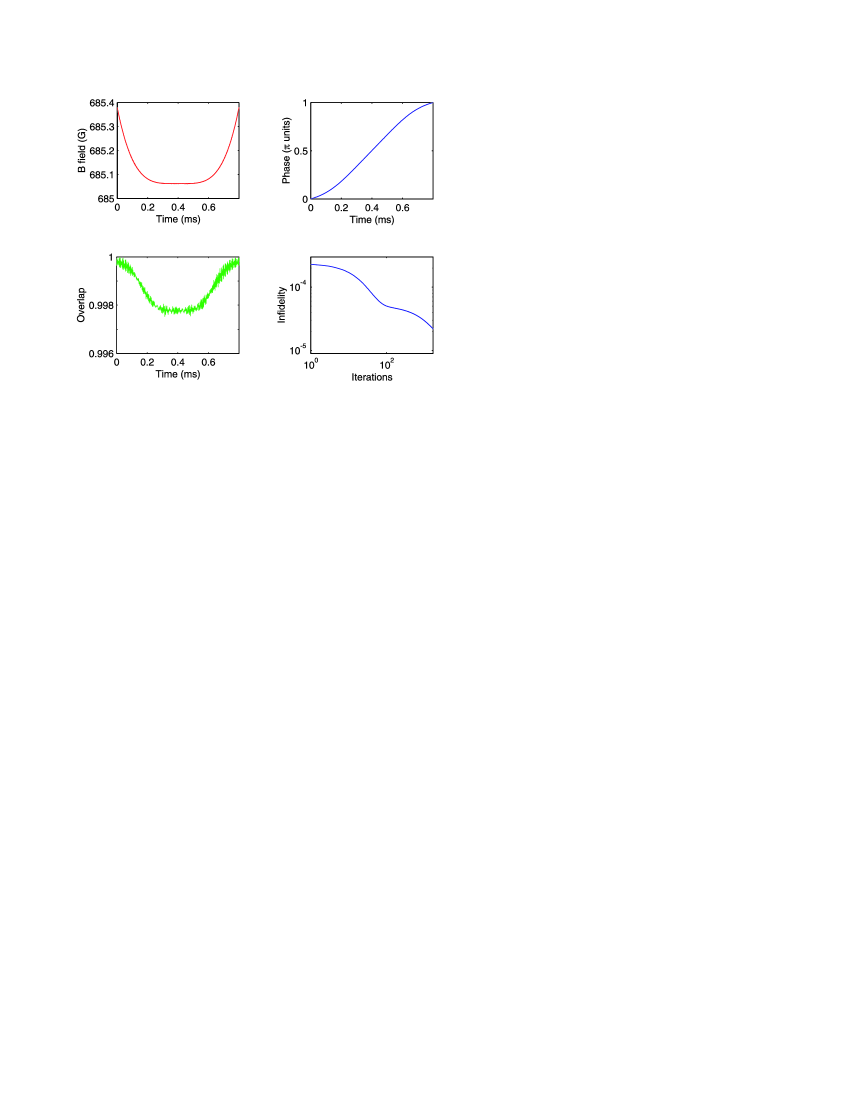
Figure 4: Two-qubit gate operation via optimal magnetic field control: optimized field time dependence (top left); overlap between initial and evolved state (bottom left); accumulated two-particle phase $\varphi$ (top right); decrease of the infidelity with increasing iterations (bottom right).

We will identify our qubit logical states with the clock-transition states

$$\left|0\right\rangle\equiv\left|F=1,m_{F}=0\right\rangle,\quad\left|1\right\rangle\equiv\left|F=2,m_{F}=0\right\rangle.$$ (12)

The main advantage of this choice is that the qubit states are not sensitive to the magnetic field, and hence not subject to decoherence due to its fluctuations. We will use the resonance for the channel $|00\rangle$ occurring around $B_{0}=685$ G, having a width $\Delta_{n}=16$ mG. For obtaining a two-qubit gate, the magnetic field is ramped across $B_{0}$, and eventually tuned out of the Feshbach resonance again, getting the following truth table for the operation:

$$|00\rangle \rightarrow e^{\mathrm{i}\varphi}|00\rangle,$$

$$|01\rangle \rightarrow |01\rangle,$$

$$|10\rangle \rightarrow |10\rangle,$$

$$|11\rangle \rightarrow |11\rangle,$$ (13)

where we included the phase $\varphi$ accumulated by state $|00\rangle$ during the ramping process due to the interaction energy shift, whose value can be adjusted by controlling the magnetic field. If $\varphi=\pi$, a C-phase gate between the two atoms is obtained. Note that laser addressing of single qubits is never required throughout the procedure.

The magnetic ramping process can be even performed non-adiabatically, provided that all population is finally returned to the trapped atomic ground state. This can be accomplished via a quantum optimal control technique in analogy with the above discussion for the transport process. The control parameter in this case is the external magnetic field $B$. Care has to be taken in optimizing not only the absolute value of the overlap of the final state onto the goal state, but also its phase $\varphi$. Fig. 4 shows the optimization results for a trap with transverse frequencies of 100 kHz and a longitudinal frequency of about 25 kHz, corresponding to the right well of Fig. 1. The final infidelity is about $2\times 10^{-5}$ in this case.

5 Outlook

We have described a scheme using moving tweezers and state-dependent controlled collisions, which is able to implement a quantum gate between two individual atoms with a high fidelity. The sensitivity of the scheme to intensity or position fluctuations has been examined, and the controlled motion is found to be very tolerant to “common-mode” noise between the two tweezers. It is even relatively tolerant to differential noise, because the overall process is close to adiabatic, and designed in such a way as to avoid unwanted level crossings.

The magnetic field which is used here to obtain the Feshbach resonance would be ultimately very advantageously replaced by an optical field [27, 28], which can be switched on and off with high speed and precision, and which will not perturb the neighboring atoms stored in the holographic array. Though the overall scheme is clearly not easy to implement, optimal control techniques as used here certainly help to make it closer to realistic.

References

- [1] D.P. Di Vincenzo, Fortschr. Phys 48, 9 (2000).
- [2] I.E. Protsenko, G. Reymond, N. Schlosser, P. Grangier, Phys. Rev. A 65, 52031 (2002).
- [3] D. Jaksch, J.I. Cirac, P. Zoller, L. Rolston, R. Côté and M.D. Lukin, Phys. Rev. Lett. 85, 2208 (2000).
- [4] G.K. Brennen, I.H. Deutsch, and P.S. Jessen, Phys. Rev. A 61, 062309 (2000).
- [5] G.K. Brennen, C.M. Caves, P.S. Jessen, and I.H. Deutsch, Phys. Rev. Lett. 82, 1060 (1999).
- [6] T. Calarco, E. A. Hinds, D. Jaksch, J. Schmiedmayer, J.I. Cirac, P. Zoller, Phys. Rev. A, 61, 22304 (2000).
- [7] D. Jaksch, H.-J. Briegel, J.I. Cirac, C. W. Gardiner, P. Zoller, Phys. Rev. Lett 82, 1975 (1999).
- [8] J. Mompart, K. Eckert, W. Ertmer, G. Birkl, M. Lewenstein, Phys. Rev. Lett 90, 147901 (2003).
- [9] K. Eckert, J. Mompart, X.X. Yi, J. Schliemann, D. Bruß, G. Birkl, M. Lewenstein, Phys. Rev. A. 66, 042317 (2002).
- [10] O. Mandel, M. Greiner, A. Widera, T. Rom, T.W. Hnsch, I. Bloch, Nature 425, 937 (2003).
- [11] N. Schlosser, G. Reymond, I. Protsenko and P. Grangier, Nature 404, 1024 (2001).
- [12] N. Schlosser, G. Reymond and P. Grangier, Phys. Rev. Lett. 89, 23005 (2002).
- [13] G. Reymond, N. Schlosser, I. Protsenko and P. Grangier, Phil. Trans. Roy. Soc. London, A 361, 1527 (2003).
- [14] D. Frese, B. Ueberholz, S. Kuhr, W. Alt, D. Schrader, V. Gomer, D. Meschede, Phys. Rev. Lett. 85, 3777 (2000).
- [15] S. Kuhr et al., Phys. Rev. Lett. 91, 213002 (2003).
- [16] R. Dumke, M. Volk, T. Müther, F.B.J. Buchkremer, G. Birkl, W. Ertmer, Phys. Rev. Lett 89, 097903 (2002).
- [17] D. Boiron, A. Michaud, J.M. Fournier, L. Simard, M. Sprenger, G. Grynberg, and C. Salomon, Phys. Rev. A 57, 4106 (1998).
- [18] D. G. Grier, Nature 424, 810-816 (2003).
- [19] S. Bergamini, B. Darquié, M. Jones, L. Jacubowiez, A. Browaeys, and P. Grangier, JOSA B 21, 1889 (2004).
- [20] J.I. Cirac, P. Zoller, Nature 404, 579 (2000).
- [21] D. Kielpinski, C. Monroe, D.J. Wineland, Nature 417 709 (2002).
- [22] T. Calarco, U. Dorner, P.S. Julienne, C.J. Williams, and P. Zoller, Phys. Rev. A 70, 012306 (2004).
- [23] C.J. Pethick and H. Smith, Bose-Einstein Condensation in Dilute Gases, Cambridge University Press, Cambridge, 2002.
- [24] J. Weiner, V.S. Bagnato, S. Zilio, and P.S. Julienne, Rev. Mod. Phys. 71, 1 (1999).
- [25] F.H. Mies, E. Tiesinga, and P.S. Julienne, Phys. Rev. A 61, 022721 (2000).
- [26] A. Marte, T. Volz, J. Schuster, S. Dürr, G. Rempe, E.G.M. van Kempen, and B.J. Verhaar, Phys. Rev. Lett. 89, 283202 (2002).
- [27] P.O. Fedichev, Y. Kagan, G.V. Shlyapnikov, and J.T.M. Walraven , Phys. Rev. Lett. 77, 2913 (1996).
- [28] M. Theis, G. Thalhammer, K. Winkler, M. Hellwig, G. Ruff, R. Grimm, and J. Hecker Denschlag, Phys. Rev. Lett. 93 123001 (2004).