Phase-space reconstruction of an atomic chaotic system

Abstract

We consider the dynamics of a single atom submitted to periodic pulses of a far-detuned standing wave generated by a high-finesse optical cavity, which is an atomic version of the well-known “kicked rotor”. We show that the classical phase-space map can be “reconstructed” by monitoring the transmission of the cavity. We also studied the effect of spontaneous emission on the reconstruction, and put limits to the maximum acceptable spontaneous emission rate.

I Introduction

The kicked rotor (KR) is a widely explored system that has a paradigmatic status in studies of classical Chirikov (1979) and quantum chaos Casati et al. (1979); Izrailev (1990). In recent years, the advent of laser cooling of atoms allowed the realization of an atomic version of the KR Graham et al. (1992); Klappauf et al. (1998), which has been used in experiments by many groups Klappauf et al. (1998); Ammann et al. (1998); Oberthaler et al. (1999); Ringot et al. (2000). This consists simply in placing laser-cooled atoms in a pulsed laser standing wave. In adequate (but rather general) conditions, the atomic center of mass motion “feels” the presence of the standing wave as an “optical potential” which varies sinusoidally in space. One can then easily modulate (with period $T)$ the light intensity in the form of short pulses to obtain a hamiltonian of the form

$$H=\frac{p^{2}}{2M}+V_{0}\cos(2k_{L}x)\sum_{n=0}^{N-1}\delta_{\tau}(t^{\prime}-nT),$$ (1)

where $M$ and $p$ are resp. the atom mass and center of mass momentum, $V_{0}$ is the amplitude of the optical potential (which is proportional to $I/\Delta$, where $I$ is the intensity of the standing wave and $\Delta$ the laser-atom detuning), $k_{L}=2\pi/\lambda_{L}$ the wave number of the standing wave (in the $x-$direction), and $\delta_{\tau}$ a square function of duration $\tau$ and amplitude $1$. In the limit $\tau\rightarrow 0$, or, more exactly, in the limit

$$\frac{\left\langle p^{2}\right\rangle^{1/2}\tau}{M}\ll\lambda_{L},$$ (2)

one can put $\delta_{\tau}/\tau\rightarrow\delta$ and one obtains exactly the hamiltonian of the KR. In order to obtain this hamiltonian in its standard form, we perform the normalizations $t^{\prime}/T\rightarrow t$, $2k_{L}x\rightarrow X$, $(2k_{L}T/M)p\rightarrow P$:

$$H=\frac{P^{2}}{2}+K\cos X\sum_{n=0}^{N-1}\delta(t-n)$$ (3)

where the only free parameter is the normalized kick strength $K=4V_{0}k_{L}^{2}T\tau/M$.

Many of the recent experimental studies were aimed at quantum aspects of the KR dynamics, as “dynamical localization” Klappauf et al. (1998); Szriftgiser et al. (2002), quantum resonances D’Arcy et al. (2001), or “chaos-assisted” tunneling Steck et al. (2001); Hensinger et al. (2001). Quantum effects in such system manifest for times larger than the “Ehrenfest time", when quantum dynamics begins to take over classical dynamics. This is the domain of “quantum chaos”, which is defined as the quantum dynamics of systems which are chaotic in the classical limit. It is well known that the quantum behavior of such systems bears little relation to the classical chaotic behavior of their classical counterparts, basically because Schrödinger equation is linear. One of the most exciting questions about quantum chaos is “How the initially classical dynamics and latter quantum dynamics diverge from one another?” Clearly, the critical point in this divergence is situated between the Ehrenfest time $t_{E}\sim T\ln(1/{\mathchar 22\relax\mkern-9.0muk})$ and the so-called “localization time" $t_{L}\sim T(K/{\mathchar 22\relax\mkern-9.0muk})^{2}$, where ${\mathchar 22\relax\mkern-9.0muk}$ is the effective Planck constant . Fortunately, in the atomic KR the parameters can be widely changed which allows one to adjust these times to experimentally convenient scales. However, even if the adequate time domain is accessible, it is still difficult to put into evidence the transition between classical and quantum regimes because, usually, the kind of measurements performed on a microscopic system is different from – and often not simply related to – the kind of measurement performed on macroscopic systems. Typically, studies of classical dynamics rely on the notion of trajectory (phase-space maps, first-return maps, Poincaré sections…) whereas studies of quantum dynamics emphasize mean quantities and probability distributions. The purpose of the present paper is to describe and study an experimentally realizable situation in which reconstruction of the atom center of mass dynamics can be done, thus reconciliating quantum- and classical-type measurements. Hopefully, such a setup would provide a better understanding of the above-mentioned transition between classical and quantum dynamics. Throughout this paper, we shall treat the atomic motion as a classical motion: we shall consider that the atomic center of mass position and momentum are enough to characterize the dynamics. This is true as long as the dynamics is essentially classical, that is, for times shorter than the localization time, or as far as the sources of decoherence – mainly spontaneous emission in the present case – act often enough to provoke a quantum coherence collapse before interference effects can develop and appreciably change the classical behavior.

II Kicked rotor dynamics

In recent years, the quality of optical cavities has been dramatically improved. It is now possible to build cavities of very high finesse Hood et al. (2000); Münstermann et al. (1999). In such a cavity, the index of refraction generated by one atom is enough to change mesurably the resonance condition, and the cavity can thus be used to “count atoms one by one” Mckeever et al. (2004). As an atom moves inside the cavity, it “probes” regions where the radiation intensity is not the same. For example, cavity modes usually have a gaussian profile, whose intensity is larger at the center than in the border. In the same way, as the field inside the cavity forms a standing wave, changing the longitudinal position of the atom also changes the intensity to which it is submitted (Fig. 1). This is the situation we shall consider in the present paper. Because of the Kerr effect, the refractive index of the atom is modified by the intensity of the radiation to which it is exposed, and the changing of the refractive index in turn changes the cavity resonance condition. By measuring the cavity transmission one can extract information on the position of the atom. This is an “autoconsistency” problem: the change in the resonance condition changes the cavity field, that in turn changes the atom refractive index. This means that the amplitude of the kicks felt by the atom will also depend on its position, which is in contradiction with the standard definition of the KR. We shall take this fact into account in our simulations, but will arrange parameters in order to make the variation of the kick strength $K$ small enough to not disturb too much the dynamics of the KR.

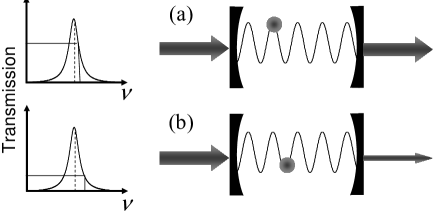
Figure 1: Schematic view of the proposed setup. If the atom is at a crest (a) or at a node (b) of the cavity electromagnetic field, the Kerr nonlinear refractive index produced is different, the resonance condition of the cavity is modified, and the transmitted intensity changes, allowing detection of the longitudinal position of the atom.

An experimental limitation that must also be taken into account is that one cannot change instantaneously the radiation intensity inside a cavity. The “lifetime” of a photon inside the cavity is roughly $\tau_{c}=L/(c\mathcal{T})$, where $\mathcal{T}$ is the (intensity) transmission coefficient of the mirrors and $L$ the length of the cavity. The duration $\tau$ of the kicks shall thus be at least of a few $\tau_{c}$. However, the validity condition for identifying the kicks with a delta function, Eq. (2), must also be satisfied. This implies that

$$\frac{2hL}{\lambda_{L}^{2}Mc}\sqrt{N}\ll\mathcal{T}$$ (4)

where we used the order of magnitude value $\left\langle p^{2}\right\rangle^{1/2}\sim 2\hbar k_{L}\sqrt{N}$ after $N$ kicks are performed . Thus given $\mathcal{T}$, there is a maximum number of kicks (i.e. a maximum duration of the experiment), $N_{max}\sim\left[\lambda_{L}^{2}Mc\mathcal{T}/(2hL)\right]^{2}$. For cesium this gives $N_{max}\sim(\mathcal{T}/L)^{2}\times 10^{9}$ m². This condition is not hard to satisfy: for $\mathcal{T}=10^{-6}$ and $L=10^{-4}$ m, $N_{max}\sim 10^{5},$ whereas experiments currently last only for a few hundred kicks.

Integrating the equations of motion obtained from Eq. (3) over one period $T=1$ produces the so-called “standard map” Chirikov (1979)

$$X_{n+1}=X_{n}+P_{n}$$ (5a)

$$P_{n+1}=P_{n}-K_{n+1}\sin X_{n+1}.$$ (5b)

where we took into account the fact that, due to the nonlinear Kerr effect, $K_{n}=K(X_{n})$: the intensity of the kick depends on the position of the atom. In constructing the phase-space portrait of the kicked rotor, it is usual to simplify the display by taking all the quantities “modulus $2\pi"$ (we shall represent the modulus $2\pi$ of a given quantity $A$ by $A[2\pi]$). This is due to the fact taht the potential is periodic in space, of period $2\pi$ in reduced units. This means that if $P_{n}=2\pi q+p$, with $p<2\pi$ and $q$ integer, then, after Eq. (5a), $X_{n+1}=X_{n}+p+2\pi q$. Thus $X_{n+1}[2\pi]=X_{n}[2\pi]+p$: the physics is the same for momenta differing by an integer multiple of $2\pi.$ We shall thus, according to the usual convention, draw phase-space maps by plotting $X[2\pi]$ vs. $P[2\pi]$. We show a typical plot of the KR phase-space in Fig. 4(a).

III Cavity dynamics

A schematic view of the proposed experiment is shown in Fig. 1. The atom is placed inside a high-finesse cavity, and its presence shifts the resonance condition of the cavity in a nonlinear way: this shift depends on the radiation intensity seen by the atom, and thus on its longitudinal position. The intensity transmitted through the cavity can thus be related to the position of the atom. However, this position is defined only with respect to the closest node; shifting the position of the atom by a period of the standing wave produces the same transmission signal .

If a laser beam of wavenumber $k_{L}$ intensity $I_{0}$ is injected into an empty Fabry-Perot cavity made of two identical mirrors a distance $L/2$ apart, of transmission coefficient $\mathcal{T}$ and reflection coefficient $\mathcal{R}=1-\mathcal{T}$, the intracavity intensity is given by the well-known Airy function

$$I_{c}=\frac{1/\mathcal{T}}{1+F^{2}\sin^{2}\left(\frac{k_{L}L_{opt}}{2}\right)}I_{0},$$ (6)

leading to a resonance Rabi frequency

$$\Omega^{2} = \Omega_{0}^{2}\cos^{2}\left(k_{L}x\right)$$ (7)

$$= \left(\frac{3\pi\Gamma}{\hbar ck_{L}^{3}}\right)\frac{1/\mathcal{T}}{1+F^{2}\sin^{2}\left(\frac{k_{L}L_{opt}}{2}\right)}I_{0}\cos^{2}\left(k_{L}x\right)$$ (8)

where $F=2\sqrt{\mathcal{R}}/\mathcal{T}$ is the finesse of the cavity divided by $\pi/2$ and $\Gamma$ the natural width of the atomic transition. The parameter $K$ [Eq. (3] turns out to be Klappauf et al. (1998):

$$K = \frac{1}{2}\omega_{r}T^{2}\frac{\Omega_{0}^{2}}{\Delta}$$

$$= \left(\omega_{r}T\right)\left(\Gamma T\right)\left(\frac{\Gamma}{\Delta}\right)\frac{1/\mathcal{T}}{1+F^{2}\sin^{2}\left(\frac{k_{L}L_{opt}}{2}\right)}\frac{I_{0}}{I_{s}}$$

where $I_{s}\equiv\hbar ck_{L}^{3}\Gamma/(6\pi)$ is the saturation intensity $\sim 2$ mW/cm² for cesium, $\omega_{r}=\hbar k_{L}^{2}/(2M)$ is the recoil frequency ($\omega_{r}/(2\pi)\sim 2$ kHz for cesium) and $\Delta$ the laser-atom detuning.

In Eq. (8), $L_{opt}=L+\Delta L$ is the optical length of the cavity, $L$ is its physical length and $\Delta L$ is the correction due to the presence of the atom:

$$k_{L}\Delta L = \frac{3\pi\Gamma}{2k_{L}^{2}L_{at}^{2}}\frac{\Delta}{\Delta^{2}+\frac{\Omega^{2}}{2}+\frac{\Gamma^{2}}{4}}$$

$$= \left(\frac{3\pi}{2k_{L}^{2}L_{at}^{2}}\right)\frac{\Delta/\Gamma}{\frac{\Delta^{2}}{\Gamma^{2}}+\frac{\Omega^{2}}{2\Gamma^{2}}+\frac{1}{4}}$$

where $L_{at}$ is the linear size of the effective volume occupied by the atom. The definition of this volume depends on the details of the experiment being performed. In the case of laser-cooled atoms, we can take this volume as the volume of the atom cloud in a magneto-optical trap, roughly $L_{at}\sim 100$ $\mu$m, which gives $3\pi/[2(k_{L}L_{at})^{2}]\sim 10^{-5}.$ For $\Delta\approx 10^{3}\Gamma$, which is a typical value, the dephasing $k_{L}\Delta L$ induced by a lone atom is roughly 10^-8, which is hard to detect directly. The effect is however enhanced by the presence of the cavity.

The detected signal is the intensity transmitted through the cavity, given by

$$S=\frac{1}{1+F^{2}\sin^{2}\left(\frac{k_{L}L_{opt}}{2}\right)}I_{0}=I_{c}/\mathcal{T}$$ (9)

which depends on the radiation intensity seen by the atom through $L_{opt}$ , and thus on the atom position. If $F\gg 1$, the half-width of the Airy peak corresponds roughly to

$$F^{2}\sin^{2}\left(\frac{k_{L}L_{opt}}{2}\right)\approx F^{2}\frac{\left(k_{L}L_{opt}\right)^{2}}{4}=1,$$ (10)

thus

$$k_{L}L_{opt}=\frac{2}{F}.$$ (11)

One easily finds

$$\left|\frac{\Delta I_{t}}{I_{0}}\right| \approx \frac{F^{2}k_{L}L}{4}\left|k_{L}\Delta L\right|=\frac{F}{2}\left|k_{L}\Delta L\right|$$

where we supposed $k_{L}L\approx 2/F$ . Then, taking $k_{L}\Delta L\approx 10^{-8}$, an experimentally realistic value Hood et al. (2000) of $F\approx 10^{6}$ produces a detectable 1%-variation of the transmitted intensity .

Techniques based on the Kerr nonlinearity similar to that proposed here have been recently used for monitoring the radial motion of an atom trapped in high-finesse cavity Hood et al. (2000); Münstermann et al. (1999). In our case, it is the longitudinal motion of the atom that should be monitored. This is complicated by the periodic character of the standing wave inside the cavity. We shall discuss in the next section the algorithm we developed to deal with this problem.

IV The reconstruction algorithm

Figure 2: First return map $S_{n}\times S_{n+1}$ for the cavity-transmission signal, with $F=10^{6}$. Structures are clearly visible, but no direct relation to the topology of the phase-space of the KR (Fig. 4a) can be drawn.

In order to reconstruct the phase-space map from the cavity transmission signal, we suppose that the transmission value corresponding to each kick $n$ is recorded, forming a temporal series $S_{n}$. The information given by the bare signal is however incomplete. Fig. 2 displays the first return map corresponding to the temporal series $S_{n}$. Its topology do not evoke at all the KR phase-space map shown in Fig. 4a. Let us consider the information that can be extracted from two successive values of the cavity transmission, $S_{1}$ at kick $1$ and $S_{2}$ at kick 2. Referring to Fig. 3, we see that the cavity transmission leaves an indeterminacy on the position, as the points $X_{1}$, $X_{1}^{\prime}$ and $X_{1}^{\prime\prime}$ correspond to the same transmission. Generally two classes of points lead to the same transmission

$$X\quad\mathrm{and}\quad X^{\prime}=X+2\pi q$$ (12a)

$$X\quad\mathrm{and}\quad X^{\prime\prime}=2\pi q-X.$$ (12b)

($q$ is an integer).

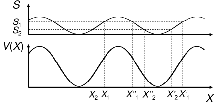
Figure 3: Correspondence between the transmission signal and the atom longitudinal position inside the cavity.

$X$	$X_{1}$	$X_{1}+2\pi q_{1}$	$2\pi q_{1}-X_{1}$
$X_{2}$	$X_{2}-X_{1}$	$X_{2}-X_{1}-2\pi q_{1}$	$X_{2}+X_{1}-2\pi q_{1}$
$X_{2}+2\pi q_{2}$	$X_{2}-X_{1}+2\pi q_{2}$	$X_{2}-X_{1}+2\pi(q_{2}-q_{1})$	$X_{2}+X_{1}+2\pi(q_{2}-q_{1})$
$2\pi q_{2}-X_{2}$	$-(X_{2}+X_{1})+2\pi q_{2}$	$-(X_{2}+X_{1})+2\pi(q_{2}-q_{1})$	$-(X_{2}-X_{1})+2\pi(q_{2}-q_{1})$

Table 1: Possible momentum ($X_{2}-X_{1})$ determinations for different choices of the position determination ($q_{1}$ and $q_{2}$ are integers). Eliminating the terms of the form $2\pi\times$(integer number), the only possibilities are $x_{2}+x_{1}$, $-(x_{2}+x_{1})$, $x_{2}-x_{1}$ and $-(x_{2}-x_{1})$, with $x_{i}=X_{i}[2\pi]$. Considering that trajectories corresponding to momenta $P$ and $-P$ are identical in the phase-space map leaves only two choices, $x_{2}+x_{1}$ and $x_{2}-x_{1}$.

However, as it is $X[2\pi]$ that is displayed in the phase-space map, the value of the integer number $q$ in Eqs. (12b) is irrelevant. This leaves us with just two possible values, $x$ and $2\pi-x$, where $x=X[2\pi]$. As the motion of the atom is free between two kicks, the momentum associated to the kick $n$ is $P_{n}=X_{n+1}-X_{n}$. Moreover, we note that $P$ and $-P$ lead to the same trajectory in the phase portrait. Introducing the relevant (for phase-portrait-plotting purposes) value $p_{n}=P_{n}[2\pi]$, we find that there are only two distinct choices for the momentum: $p_{1}=x_{2}-x_{1}$ or $p_{1}=x_{2}+x_{1}$ (see table 1). We must thus chose arbitrarily one of the two. If we now include the next value $x_{3}$ of the position (with its own arbitrary choice of the determination), we can deduce in the same way a value for $p_{2}$. But Eq. (5b) implies that the successive values $p_{1}$ and $p_{2}$ of the momentum must satisfy

$$p_{2}=p_{1}-\left(K_{2}\sin x_{2}\right)[2\pi],$$ (13)

which allows us to test the coherence of the choices.

In practice, our algorithm proceeds as follows: i) For each point $S_{n}$ in the time series of cavity transmission, we first estimate a value for the intracavity intensity $I_{c}^{(0)}$ using Eq. (6) with $L_{opt}=L$. This value of $I_{c}^{(0)}$is then used to estimate the atom position $x_{n}^{(0)}$ and to calculate a first correction to $L$, $L^{(1)}=L+\Delta L_{1}$, which in turn is used to determine a corrected value $I_{c}^{(1)}$ and a corrected value of the position $x_{n}^{(1)}$. The process is iterated until it converges to produce the value of the position corresponding to the $n^{th}$ kick, $x_{n}$. Ten steps are usually enough to insure the convergence of the process. ii) We choose arbitrarily between the two possible determinations $x_{n}$ or $2\pi-x_{n}$ of the position and calculate the corresponding value of $p_{n}$ (choosing arbitrarily between $x_{n}-x_{n-1}$ and $x_{n}+x_{n-1}$). iii) Each time three successive momentum values have been determined, we use Eq. (13) to test the coherence of the choices. If this condition is violated, we recalculate the last three points with a different choice of the position determinations. iv) Once a trajectory is reconstructed, one starts again with another time series corresponding to another set of initial conditions.

Fig. 4 compares the exact KR phase-space map with the reconstructed one. We see that the agreement is good. The number of restarts due to the coherence test is 380 over 3000 data points.

Figure 4: Comparison between the original (a) and the reconstructed (b) KR phase space-map. Parameters are $K=0.8$, $F=10^{6}$. Larger structures are easier to reconstruct than smaller ones.

V Effect of the spontaneous emission

The good reconstruction obtained in the preceding section is however impossible to achieve in a real experiment, because of the unavoidable presence of spontaneous emission in the system. However, the spontaneous emission rate can be controlled – to a certain extent – in such systems, because it roughly scales with the inverse of the square of the laser-atom detuning, whereas the optical potential amplitude $V_{0}$ scales with the inverse of the detuning; one can thus adjust the parameter in such way that spontaneous emission level is tolerable during the experiment duration. In the one dimensional situation we are considering, the effect of spontaneous emission is to add to the value of $p$ in the average a unit of photon momentum $\pm\hbar k_{L}$ (corresponding to ${\mathchar 22\relax\mkern-9.0muk}/2=2\hbar k_{L}^{2}T/M$ in reduced units), with an arbitrary sign, each time it happens. We introduced spontaneous emission in our simulations by a simplified Monte-Carlo procedure. For each pulse of duration $\tau$, we calculate the probability for a fluorescence cycle to happen

$$g_{a}=\frac{\Gamma}{2}\frac{\Omega^{2}/2}{\Delta^{2}+\frac{\Omega^{2}}{2}+\frac{\Gamma^{2}}{4}}\tau.$$ (14)

We suppose that this probability is less than one, that is, there is at most one fluorescence cycle per pulse. A random number $0\leq\alpha_{a}<1$ is picked, and if $\alpha_{a}<g_{a}$ the atom performs a fluorescence cycle. In such case, another number $\eta_{a}$ taking randomly one of two possible values $-{\mathchar 22\relax\mkern-9.0muk}/2$ and $+{\mathchar 22\relax\mkern-9.0muk}/2$ is picked to decide of the direction of the recoil of the atom . The atom decay back to the ground state produces a new recoil in a random direction given by another random number $\eta_{sp}=\pm{\mathchar 22\relax\mkern-9.0muk}/2$. We suppose that $T\gg\Gamma^{-1}$ , so that, with respect to the atom dynamics, the whole fluorescence cycle can be considered as instantaneous. The effect of the spontaneous emission during the $n^{th}$ kick is thus to change the momentum $p_{n}\rightarrow p_{n}+\left(\eta_{a}+\eta_{sp}\right)$. This change in the momentum displaces the point corresponding to the $p_{n}$ in the phase-space of a quantity that can be as large as ${\mathchar 22\relax\mkern-9.0muk}[2\pi]$, compared to the width of the map $2\pi$. The effect of spontaneous emission thus increases as the effective Planck constant ${\mathchar 22\relax\mkern-9.0muk}$ of the system increases, that is, as the system becomes more “quantum”. Fortunately, the classical type of dynamics we are interested in here corresponds to ${\mathchar 22\relax\mkern-9.0muk}<1$.

Fig. 5 compares the phase-space reconstruction obtained with different values of $g_{a}$. The number of restarts due to bad choices of position/momentum determinations was typically two times larger than in the absence of spontaneous emission. We can estimate the maximum spontaneous emission rate per kick still allowing the reconstruction of the phase map as $g_{max}\sim 0.05$, which means that, in order to perform this experiment, the parameters should be chosen so that the localization time be of the order of $t_{L}\sim g_{max}^{-1}\sim 20$ kicks. However, 20 kicks are not enough to produce a good phase space portrait; a better combination of parameters would be, e.g., $g\sim 0.01$ and $t_{L}\sim 100$. This values are still compatible with current experimental values.

Figure 5: Influence of the spontaneous emission in the phase-space reconstruction. Parameters are $K=0.8$ and $F=10^{6}$.

VI Conclusion

We have proposed and numerically tested a method allowing reconstruction of the classical dynamics of the “atom-optics” kicked rotor formed by an atom exposed to pulses of an intracavity standing wave. We have discussed the relevant parameters of the system and showed that they can fit with real experimental situations. Our method can be used to probe interesting phenomena, like the transition from the classical dynamics to the quantum dynamics as the spontaneous emission rate becomes smaller than the inverse of the localization time.

It is rather difficult to guess what will happen when this limit is approached. In the quantum case, the atom cannot be characterized by a single point in the phase space. This means that the spreading of the wavefunction must be considered, and the classical notion of trajectory is not any more a good one. In particular, the the cavity transmission will be affected by the spatial spreading, as it allows the atom to “probe” different intensity regions. One must also consider the decoherence effect of spontaneous emission that reduces the wavepacket if it happens often enough. An interesting way to explore such situation is to compare a Wigner-function picture of the quantum phase-space in presence of decoherence with the classical map Carvalho et al. (2004). If the present method proves able to experimentally explore the classical/quantum transition, it would be highly valuable for studies of the nontrivial relation between classical and quantum chaos.