Transition From Quantum To Classical Mechanics As Information Localization

Abstract

Quantum parallelism implies a spread of information over the space in contradistinction to the classical mechanical situation where the information is ”centered” on a fixed trajectory of a classical particle. This means that a quantum state becomes specified by more indefinite data. The above spread resembles, without being an exact analogy, a transfer of energy to smaller and smaller scales observed in the hydrodynamical turbulence. There, in spite of the presence of dissipation (in a form of kinematic viscosity), energy is still conserved. The analogy with the information spread in classical to quantum transition means that in this process the information is also conserved. To illustrate that, we show (using as an example a specific case of a coherent quantum oscillator) how the Shannon information density continuously changes in the above transition . In a more general scheme of things, such an analogy allows us to introduce a ”dissipative” term (connected with the information spread) in the Hamilton-Jacobi equation and arrive in an elementary fashion at the equations of classical quantum mechanics (ranging from the Schrödinger to Klein-Gordon equations). We also show that the principle of least action in quantum mechanics is actually the requirement for the energy to be bounded from below.

Keywords: Classical to quantum transition; information density transformation

1 INTRODUCTION

Present day efforts in making quantum computing a reality are centered mainly on harnessing immense parallelism (e.g., entangled states) inherent in quantum mechanics. In terms of information content such a parallelism means that information is spread over the whole space. The implication is that information density is not delta-function-like ( as in a classical case) but is represented by a ’broader’ function. In a sense, this can be interpreted as an information spread, in contradistinction to a classical case, where the information is centered around the well-defined path determined by the classical equations of motion. The problem of extracting the information so spread becomes central to every possible quantum computer. Therefore it seems important to determine how this spread of information occurs in general.

For the first time an idea about a ”spread” of information in a transition from the classical to the quantum world was expressed by P.Dirac more than 70 years ago [1]. He wrote, ”The limitation in the power of observation puts a limitation on the number of data that can be assigned to a state. Thus a state of an atomic system must be specified by fewer or more indefinite data than a complete set of numerical values for all the coordinates and velocities at some instant of time.” Unfortunately, he did not elaborate further on this idea.

Does all this mean that information is lost via some sort of dissipation in a transition from classical to quantum case? In another words, is information lost in a literal sense of the word, or simply ’spread around’, that is the respective information density undergoes a change in a transition from a classical to quantum case? The mechanism of the latter represents what we would call the $information~{}spread$. As will be shown below, this $information~{}spread$ is the correct answer.

A tentative approach to find the answer to this problem in a general way was outlines at [2]. There we observed that contrary to the conventional point of view (regarding the transition from classical to quantum physics as being necessarily due to decoherence [3]), our investigation of a superfluid state demonstrated coherence preservation. Indeed, in our view decoherence plays essentially no role in the transition from ordinary classical physics to quantum physics. This transition can occur in a continuous fashion preserving the coherence in a classical state.

We also argued that ”Whereas the entropy of any deterministic classical system described by a principle of least action is zero, one can assign a ”quantum information” to quantum mechanical degree of freedom equal to Hausdorff area of the deviation from a classical path.” This raises an interesting problem of realization of a quantum computer based on a continuous transition from a quantum coherent state to a classical coherent state. Such an approach is contrary to the conventional treatment of quantum computing where quantum coherence is destroyed by classical measurements. The difficulty of preserving quantum coherence lies at the heart of the general difficulty of realizing such a computer.

In what follows we demonstrate (using a coherent state of a quantum oscillator) how the information-preserving mechanism, characterized by a spatial spread of information density, occurs. In a sense (and only in a sense), this mechanism is analogous to the effect of dissipation on the velocity profile of a viscous fluid, illustrated, for example, by Stokes’s first problem about a suddenly accelerated plane wall immersed in a viscous fluid [4]. We write ” in a sense”, since in contradistinction to fluid mechanics ( where the system dissipates energy), here no loss of information occurs.

Such an analogy allows us to show how in a $general$ scheme of things (not restricted to some special cases as in [6]) the addition of the specific ”dissipative” term (similar to the dissipative term in fluid mechanics) to the classical equations of motion will lead in a natural way to the wave equations, ranging from the Schr$\mathrm{\ddot{o}}$dinger to Klein-Gordon, to Dirac equations .

If we consider the Shannon information for the coherent state of a quantum oscillator then we will be able to explicitly illustrate how the information density associated with this oscillator continuously changes from a function spread over the whole spatial domain in quantum case to the delta-function centered on the domain occupied by the values of the spatial coordinate (that is $x=acos\omega t$) allowed by classical mechanics. In particular, this proves (in full agreement with the above arguments) that in fact the $total$ information is not lost, but rather a change of its space density occurs.

2 Information Density in Classical and Quantum Regimes

Let us consider the Shannon information $I$

$$I=-\sum_{i=0}^{N}p_{i}log_{2}p_{i}$$ (1)

Here $p_{i}$ is the probability of an event $A_{i}$. In what follows we replace $log_{2}$ by the natural logarithm which is not going to change the meaning of the information, but will simply introduce a non-essential numerical factor. For our purposes we define the probability in (1) with the help of the probability density function $\Psi(x,t)$, as it is used in quantum mechanics.

In this context the probability $p_{i}$ (defining a probability of finding a particle in the space interval $x_{i},x_{i+1}$) can be written as follows

$$p_{i}=\int_{x_{i}}^{x_{i+1}}|\Psi|^{2}dx$$ (2)

Therefore

$$p_{i}Lnp_{i}=\int_{x_{i}}^{x_{i+1}}|\Psi|^{2}dx~{}Ln(\int_{x_{i}}^{x_{i+1}}|\Psi|^{2}dx)$$ (3)

For a coherent state of a quantum oscillator (3) yields:

$$p_{i}Lnp_{i}=\\ \frac{\alpha}{\sqrt{\pi}}\int_{x_{i}}^{x_{i+1}}e^{\alpha^{2}(\tilde{x}-cos\omega t)^{2}}d\tilde{x}Ln\{\alpha\int_{x_{i}}^{x_{i+1}}e^{\alpha^{2}(\tilde{x}-cos\omega t)^{2}}d\tilde{x}\}$$ (4)

where $\alpha=a\sqrt{{m\omega}/{\hbar}}$, $m$ is particle’s mass, $a$ is the classical amplitude, $\omega$ is the classical frequency and $\tilde{x}=x/a$ is the dimensionless coordinate. Parameter $\alpha$ has a clear physical meaning. Since

$$\frac{\hbar}{ma\omega}=\lambda_{db}$$ (5)

(where $\lambda_{db}$ is the respective DeBroglie wavelength),

$$\alpha=\frac{a}{\lambda_{db}}$$

indicates whether particle dynamics is a classical ($\alpha\gg 1$) or a quantum one ($\alpha\sim 1$).

Integrating (4), we obtain

$$p_{i}Lnp_{i}=\frac{1}{2}[\Phi(\alpha y_{i+1})-\Phi(\alpha y_{i})]Ln\{[\Phi(\alpha y_{i+1})-\Phi(\alpha y_{i})]\}$$ (6)

Here $y=\tilde{x}-cos\omega t$ and

$$\Phi(y)=\frac{2}{\sqrt{\pi}}\int_{0}^{y}e^{-z^{2}}dz$$

We consider a situation where

$$y_{i+1}-y_{i}=\Delta y_{i}\ll 1$$

Inserting this in (6) we arrive at the following

$$p_{i}Lnp_{i}=-\frac{1}{\sqrt{\pi}}e^{-(\alpha y_{i})^{2}}\{1+\frac{Ln\pi}{2}+(\alpha y_{i})^{2}\}\alpha\Delta y_{i}+O[(\Delta y_{i})^{2}]$$ (7)

where we use

$$xLnx_{(x\rightarrow 0)}\rightarrow-x$$

Therefore (1) becomes

$$-\sum_{i=0}^{N}p_{i}Lnp_{i}=\frac{1}{\sqrt{\pi}}\sum_{i=0}^{N}e^{-(\alpha y_{i})^{2}}\{1+\frac{Ln\pi}{2}+(\alpha y_{i})^{2}\}\alpha\Delta y_{i}$$ (8)

In the limit $N\rightarrow\infty,\Delta y_{i}\rightarrow dy$ relation (8) yields the following integral

$$-\sum_{i=0}^{N}p_{i}Lnp_{i}=\frac{1}{2\sqrt{\pi}}\int_{-\infty}^{\infty}e^{-(\alpha y_{i})^{2}}\{1+\frac{Ln\pi}{2}+(\alpha y_{i})^{2}\}\alpha dy$$ (9)

Therefore the integral function

$$\frac{dI}{dx}=\frac{\alpha}{2\sqrt{\pi}}e^{-(\alpha y_{i})^{2}}\{1+\frac{Ln\pi}{2}+(\alpha y_{i})^{2}\}$$ (10)

represents the $space~{}information~{}density$, that is the information (per unit of dimensionless length) about finding the particle at a certain location $x$. The graph of this function for various values of $a/\lambda_{db}=1,2,...,10$ is shown in Fig.$1$.

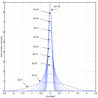
Figure 1: Information density ( per unit of dimensionless length $\tilde{x}$) as a function of $\tilde{x}-cos\omega t$ for different values of $a/\lambda_{db}=1,2,...,10$

In the limit of $\alpha=a/\lambda_{db}\rightarrow\infty$ the space information density tends to the delta-function. This indicates the onset of a purely classical regime, such that outside the region $x=acos\omega t$ (occupied by the displacement of the classical oscillator) the information density is 0. Thus all the information is ”concentrated” in the region $x-acos\omega t=0$.

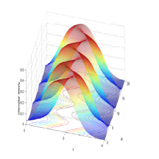
Figure 2: Information density ( per unit of dimensionless length $\tilde{x}$) as a function of $\tilde{x}$ and $t$ for $a/\lambda_{db}=.5$

In the opposite limit $\alpha=a/\lambda_{db}\rightarrow 1$ the information density function is spread over the domain $-\infty<y<\infty$ of all possible values of $x-acos\omega t$ reaching outside the region occupied by the displacement of the classical oscillator. This indicates a quantum regime characterized by the information which is not ”concentrated” on a well defined path (of measure zero) but is rather ”diffused”. This, of course, does not mean that the information is lost. On the contrary, the information is preserved, being however ”spread” over the whole space.

It is instructive to provide the graphs of the information density as a function of the spatial and temporal coordinates. These graphs are presented in Figures $2$, $3$, and $4$ for the ratios $a/\lambda_{bd}=0.5,5,15$ respectively.

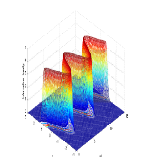
Figure 3: Information density ( per unit of dimensionless length $\tilde{x}$) as a function of $\tilde{x}$ and $t$ for $a/\lambda_{db}=5$

Once again, one can easily see that with the increase of the ratio $a/\lambda_{db}$, that is the approach to the classical regime, the information density tends to be concentrated along the classical path $\tilde{x}=cos(\omega t)$.

Here we must emphasize that the spatial information spread expressed in terms of $\bf spatial$ information density refers $exclusively$ to the Schr$\mathrm{\ddot{o}}$dinger representation of quantum mechanics. It describes the respective dynamics in spatial-temporal terms with the help of the quantum ”potential”, the wave function $\Psi(x,t)$. On the other hand, the equivalent second quantization representation of quantum mechanics deals only with the number states, without reference to their spatial distribution. Therefore it is important to find out how the respective information density varies with changes in number states, which can be quite different from the changes of information density in the Schr$\mathrm{\ddot{o}}$dinger representation.

2.1 Information Density for a Coherent State of the Quantum Oscillator in the Number State Representation

Let us calculate this information density. The probability to find an oscillator in the $n-th$ state is

$$P(n,<n>)=\frac{<n>^{n}}{n!}e^{-<n>}$$ (11)

where the average number of states

$$<n>=\frac{(m\omega^{2}<x>^{2}+<p^{2}>/m)/2}{\hbar\omega}$$ (12)

The Shannon information is then

$$I=-\sum_{n}P_{n}LnP_{n}=<n>(1-Ln<n>)+e^{-<n>}\sum_{n}\frac{<n>^{n}}{n!}Ln(n!)$$ (13)

where we use natural logarithm, instead the one base $2$, which would introduce into the result a nonessential numerical factor. From Eq.(13) follows

$$\frac{dI}{d<n>}=e^{-<n>}\sum_{n}\frac{<n>^{n}}{n!}Ln(n+1)-Ln(<n>)$$ (14)

In general, the sum in (14) cannot be found in a closed form. However, we can evaluate it in the quantum limit $<n>\ll 1$

$$\lim_{n\ll 1}=-Ln<n>\gg 1$$ (15)

Since there is no analytical solution to (14), the numerical evaluation allows us to represent the result as a graph $dI/d<n>=f(<n>)$. It is shown in Fig. $5$. One can easily see that the number state information density $decreases$ in a transition from a quantum to a classical regime, in contradistinction to the $spatial$ information density with its sharp increase around the classical trajectory.

The apparent paradox is resolved by observing that in the number state representation the Shannon information is not conserved anymore. In fact, according to (13) it increases in a transition from the quantum to the classical case, since the average number of states given by 12 (i.e. roughly the ratio of a classical amplitude and the respective De Broglie wavelength) monotonically increases. Therefore the two representations conceptually differ in this respect.

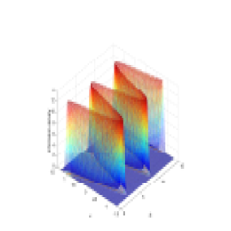
Figure 4: Information density ( per unit of dimensionless length $\tilde{x}$) as a function of $\tilde{x}$ and $t$ for $a/\lambda_{db}=15$

Figure 5: Number state information density as a function of the average number of states $<n>$

3 Schr$\mathrm{\ddot{o}}$dinger Equation as a Result of Information Spread

The previous sections imply that a judicious introduction of a ”dissipative” (or rather quasi-dissipative) term (signaling a $spatial$ spread of information) into the equations of classical mechanics can result in the respective quantum equations. To achieve this goal we use the following experimental facts:

1) Quantum phenomena are characterized by the superposition principle, implying that in contradistinction to the classical mechanics with its non-linear equations, the respective quantum equations must be linear.

2)There exists a smallest finite quantum of energy $E=\hbar\omega$, which in the phase space corresponds to the finite elemental area $\hbar$.

3) Quantum phenomena exhibit both particle and wave properties.

We begin with the second law of Newton for a single particle moving from p.$A$ to p.$F$ (see Fig.$6$). The particle can do that by taking any possible path connecting these two points. Therefore for any fixed moment of time, say $t=1$ particle’s momentum would depend on the spatial coordinate, that is $\vec{p}=\vec{p}(\vec{x},t)$. This means that now the substantial derivative $d/dt=\partial/\partial t+v_{j}\partial/\partial x_{j}$. In a sense, instead of watching the particle evolution in time one watches the evolution of its momentum in space and time. This situation is analogous to the Euler’s description of motion of a fluid (an alternative to the Lagrange description). The other way to look at that is to consider a ”flow” of an ”elemental” path and describe its ”motion” in terms of its coordinates and velocity.

Figure 6: A few paths of a path set connecting the initial and the final points traveled by a particle in $t=3sec$. It is clearly seen that particle’s velocity ( momentum) is a function of both coordinate $x$ and time $t$

Taking this into account we write the second law as follows (e.g.,[13])

$$\frac{dp_{j}}{dt}=-\frac{\partial\Pi_{jk}}{\partial x_{k}}$$ (16)

where $\Pi_{jk}$ is the momentum flux density tensor, and we adopt the convention of summation over the repeated indices.

In a purely classical case

$$\Pi_{jk}=U\delta_{jk}$$

where $U$ is the potential, representing an absence of ”friction” between different possible paths. On the other hand, at the micro-level we postulate a ”viscous” transfer of momentum from a path with a greater momentum to paths with a smaller momentum, similar to a transfer of energy from larger to smaller scales in a turbulent motion. Therefore we add to the ”ideal” momentum flux $P_{jk}$ in (16) a term analogous to the one used in classical mechanics of fluids. This yields the following expression for $\Pi_{jk}$(e.g.,[9])

$$\Pi_{jk}=U\delta_{jk}-\nu_{1}^{q}(\frac{\partial p_{j}}{\partial x_{k}}+\frac{\partial p_{k}}{\partial x_{j}}-\frac{2}{3}\delta_{jk}\frac{\partial p_{l}}{\partial x_{l}})-\nu_{2}^{q}\delta_{jk}\frac{\partial p_{l}}{\partial x_{l}}$$ (17)

where ”viscosities” $\nu_{1}^{q},\nu_{2}^{q}$ will be determined in what follows.

Inserting (17) in (16) we obtain in vector notations:

$$\frac{\partial\vec{p}}{\partial t}+\frac{1}{m}(\vec{p}\centerdot\nabla)\vec{p}=-\nabla U+\nu_{1}^{q}\nabla^{2}\vec{p}+(\frac{1}{3}\nu_{1}^{q}+\nu_{2})\nabla div\vec{p}$$ (18)

Application of $curl$ to both sides of (18) results in the following:

$$\frac{\partial}{\partial t}\nabla\times\vec{p}-\frac{1}{m}\nabla\times[\vec{p}\times(\nabla\times\vec{p})]-\nu_{1}^{q}\nabla\times[\nabla\times(\nabla\times\vec{p})]=0$$ (19)

Equation (19) is identically satisfied if $\nabla\times\vec{p}=0$, or equivalently

$$\vec{p}=\nabla S^{(q)}$$ (20)

where $S^{(q)}$ is a new ”effective action”.

It must be said, that this ”effective action” serves only as an interim auxiliary function without a clear physical meaning, which allows us to make a transition to the quantum case. Importantly enough, in contradistinction to the conventional hydrodynamical treatment of viscous fluid, the present case is irrotational. In conventional hydrodynamics of incompressible viscous fluids (with $div\vec{v}=0$) motion with $curl\vec{v}=0$ represents a potential motion $\nabla^{2}\vec{v}=0$. However at the atomic scales $\nabla^{2}S\neq 0$, because of the absence of continuity equation analogous to the one in incompressible fluid, that is now $div\vec{p}\neq 0$

Substituting(20) in (18) and using the vector identities

$$(\vec{u}\centerdot\nabla)\vec{u}\equiv\frac{1}{2}[\nabla(\vec{u}\centerdot\vec{u})-\vec{u}\times curl\vec{u}]$$

$$\nabla^{2}\vec{u}\equiv\nabla(\nabla\centerdot\vec{u})-\nabla\times(\nabla\times\vec{u})$$

we obtain the following equation

$$\nabla\{\frac{\partial S^{(q)}}{\partial t}+\frac{1}{2m}(\nabla S^{(q)})^{2}+U-\nu^{q}\nabla^{2}S^{(q)}\}=0$$ (21)

where

$$\nu^{q}=\frac{4}{3}\nu_{1}^{q}+\nu_{2}^{q}$$

Equation (21) is identically satisfied if

$$\frac{\partial S^{(q)}}{\partial t}+\frac{1}{2m}(\nabla S^{(q)})^{2}+U=\nu^{q}\nabla^{2}S^{(q)}$$ (22)

We have arrived at what can be called a modified Hamilton-Jacobi equation with ”dissipation”. As we have already indicated, it does not play any role at the macro-scales of classical mechanics due to the smallness of the dissipative term as compared to the rest of the terms. As will be shown later, this smallness is directly related to the ratio of the DeBroglie wavelength and the characteristic length on a classical scale.

Since the obtained equation is non-linear, it cannot be used to describe quantum phenomena, since this contradicts the experimental facts about superposition of quantum states. In addition, (22) does not have a wave solution, which again contradicts the experimental facts about quantum phenomena. Therefore we have (if possible) to identically transform (22) into an equation which would be

• a) linear

  and

• b) would allow wave solutions.

Requirement $b)$ can be achieved (at least for a time dependence), if it would be possible to transform (22) into a homogeneous (but still nonlinear) partial differential equation of order $2$. To test this proposition we introduce a new function, say $\Psi(\vec{x},t)$, such that

$$S^{(q)}=S^{(q)}(\Psi)$$ (23)

Inserting (23) in (22) we obtain:

$$\frac{dS^{(q)}}{d\Psi}\frac{\partial\Psi}{\partial t}+\frac{1}{2m}(\frac{dS^{(q)}}{d\Psi})^{2}(\nabla\Psi)^{2}+U=\nu^{(q)}[\frac{dS^{(q)}}{d\Psi}(\nabla\Psi)^{2}+\frac{d^{2}S^{(q)}}{d\Psi^{2}}\nabla^{2}\Psi]$$ (24)

Amazingly enough, this equation becomes a homogenous nonlinear partial differential equation of order $2$ with respect to the new function $\Psi$, if and only if the functional dependence (23) is as follows:

$$\frac{dS^{(q)}}{d\Psi}=\frac{A}{\Psi}$$ (25)

Solving (25) we obtain:

$$S^{(q)}=ALn\Psi+B$$ (26)

where constant $A$ a will be determined later with the help of the requirements formulated at the beginning of this section. Since constant $B$ does not enter into the resulting equation with respect to function $\Psi$, we set it equal to 0 without any loss of generality. Therefore (26) yields

$$S^{(q)}=ALn\Psi$$ (27)

This relation is exactly what Schr$\mathrm{\ddot{o}}$dinger originally introduced ”by hand” in his first paper in the historical series of $6$ papers on the wave equation [10].

Meanwhile we substitute (25) in (24) and obtain:

$$\frac{1}{A}\Psi\frac{\partial\Psi}{\partial t}+\frac{1}{2m}(\nabla\Psi)^{2}+\frac{1}{A^{2}}U\Psi^{2}=\frac{1}{A}\nu^{(q)}[\Psi\nabla^{2}\Psi-(\nabla\Psi)^{2}]$$ (28)

It is clear that for a particular case of the function $U$ being time-independent, (28) allows a solution proportional to $exp(i\omega t)$.

To convert (28) into a linear equation we have to ”get rid” of the nonlinear term $(\nabla\Psi)^{2}$. Since the ”viscosity” $\nu^{(q)}$ was introduced in such a way that its exact value was undetermined, we can use this fact and eliminate the nonlinear term by the appropriate choice of $\nu^{(q)}$. This procedure yields:

$$\nu^{(q)}=\frac{A}{2m}$$ (29)

As a result, equation (28) becomes

$$A\frac{\partial\Psi}{\partial t}-\frac{A^{2}}{2m}\nabla^{2}\Psi+U\Psi=0$$ (30)

We still need to find the value of constant $A$. This can be done by using the experimental fact about a smallest amount of energy available at the microscale (condition $2$ of this section). To this end we consider the relativistic Hamilton-Jacobi equation for a massless particle (in itself a rather strange, but still valid, concept within the framework of classical mechanics):

$$(\frac{\partial S}{\partial t})^{2}-(\nabla S)^{2}=0$$ (31)

where we set the speed of light $c=1$.

One can easily see that it has two different solutions. One, let’s call it particle-like, is

$$S_{p}=-Et+\vec{p}\centerdot\vec{x}$$ (32)

Another one, let’s call it wave-like, is

$$S_{w}=exp[-i(\omega t-\vec{k}\centerdot\vec{x})]$$ (33)

On one hand, from (32)

$$\frac{\partial S_{p}}{\partial t}=-E$$ (34)

and from (33)

$$\frac{\partial}{\partial t}(\frac{1}{i}LnS_{w})=-\omega$$ (35)

On the other hand, according to Planck’s hypothesis about a discrete character of energy transfer, we replace in (34) (for a single massless particle) energy $E$ by $\hbar\omega$, which yields

$$\frac{\partial}{\partial t}(\frac{S_{p}}{\hbar})=-\omega$$ (36)

From equations (35) and (36) immediately follows the unique relation between two solutions, $S_{p}$ and $S_{w}$:

$$S_{p}=\frac{\hbar}{i}LnS_{w}\equiv\frac{\hbar}{i}Ln\Psi$$ (37)

As an additional bonus, by comparing

$$\nabla S_{p}=\vec{p}$$

and

$$\nabla(\frac{1}{i}LnS_{w})=\vec{k}$$

we find from (37) the De Broglie formula

$$\vec{p}=\hbar\vec{k}$$ (38)

Thus the dual character ( wave-like and particle-like) of a solution to the Hamilton-Jacobi equation inevitably leads to the emergence of the $complex-valued$ wave ”action” $S_{w}$ (wave function $\Psi$) related to the particle action $S_{p}$ via a naturally arising substitution (37).

A comparison of (27) and (37) allows us to determine the value of constant $A$ in (27):

$$A=\frac{\hbar}{i}$$ (39)

which means that the relation between the auxiliary function $S^{(q)}$ and the function reflecting both particle and wave-like character of the phenomena on a microscale is

$$S=\frac{\hbar}{i}Ln\Psi$$ (40)

The obtained relation provides $a~{}priori$ the physical justification of the substitution (27) used by Schr$\mathrm{\ddot{o}}$dinger.

If we use constant $A$ from equation (39) in (29), we obtain the unique value of the ”viscosity” $\nu^{(q)}$:

$$\nu^{(q)}=\frac{\hbar}{2im}$$ (41)

Now it becomes clear why we call $\nu^{(q)}$ a ”viscosity”: $\hbar/m$ has a dimension of kinematic viscosity. Inserting (39) in the linear equation (30) we arrive at the Schr$\mathrm{\ddot{o}}$dinger equation:

$$i\hbar\frac{\partial\Psi}{\partial t}=-\frac{\hbar^{2}}{2m}\nabla^{2}\Psi+U\Psi$$ (42)

Here we have to make one more comment. As we have pointed earlier, the dissipative term, heuristically introduced into the Hamilton-Jacobi equation, does not play any role at the classical scales. One can consider it as small perturbations which become significant only at the micro-scales. This proposition is confirmed by the following reasoning. Smallness of the dissipative term as compared with the rest of the terms in either Hamilton-Jacobi equation (22) or the second law of Newton [written as (18)] is determined by its comparison on a dimensional basis with the dynamic term $p^{2}/mL$. The ”viscous” term is

$$\frac{\hbar p}{mL^{2}}\sim\lambda_{db}\frac{p^{2}}{mL^{2}}$$

(where $L$ is the characteristic length and $\lambda_{db}=\hbar/p$ is the De Broglie wavelength). The ratio of the latter and the former

$$\lambda_{db}/L$$

becomes negligible, when we are dealing with classical phenomena. This is fully consistent with treating a classical path as a geometrical optics limit $\lambda\rightarrow 0$ of the wave propagation.

Interestingly enough, the introduction of the ”dissipative” term (in a form of small perturbations) into the classical equations of motion (with a subsequent transition to a probabilistic description) is compatible with $fractalization$ of the deterministically defined classical path (one-dimensional curve) which gradually degenerates into a quantum fuzzy ”path”, whose Hausdorff dimension is $2$ [2, 11, 12].

Now establishing the fruitfulness of our approach, we can apply it to more complicated forms of the Hamilton-Jacobi equation. First, we introduce the dissipative term into the Hamilton-Jacobi equation for a charged particle in an electro-magnetic field

$$\frac{\partial S}{\partial t}+\frac{1}{2m}(\nabla S-e\vec{A})^{2}+e\phi=0$$ (43)

where $\vec{A}$ and $\phi$ are the vector and scalar potentials respectively.

When we follow the procedure outlined above, we must keep in mind, that now instead of the definition of momentum $\vec{p}=\nabla S$ we have to use the generalized momentum $\vec{p}=\nabla S-e\vec{A}$:

$$\frac{\partial S}{\partial t}+\frac{1}{2m}(\nabla S-e\vec{A})^{2}+e\phi=\nu^{q}\nabla\centerdot(\nabla S-e\vec{A})$$ (44)

where the ”viscosity” $\nu^{(q)}$ to be determined. Using substitution (40) in (44) and performing some elementary vector operations we arrive at the following

$$\Psi\{-i\hbar\frac{\partial\Psi}{\partial t}+\frac{1}{2m}(e^{2}A^{2}\Psi-2\frac{\hbar}{i}e\vec{A}\centerdot\nabla\Psi)+e\phi\Psi-$$

$$\nu^{q}(\frac{\hbar}{i}\nabla^{2}\Psi-e\Psi\nabla\centerdot\vec{A})\}+(\nabla\Psi)^{2}(\nu^{q}\frac{\hbar}{i}-\frac{\hbar^{2}}{2m})=0$$ (45)

By requiring this equation to be linear we get the following value of constant $\nu^{q}$

$$\nu^{q}=i\frac{\hbar}{2m}$$

which is exactly the same (Eq.41) as in the previous case of the Schr$\mathrm{\ddot{o}}$dinger equation for an electrically neutral particle. Inserting this value back in (3) we arrive at the respective Schr$\mathrm{\ddot{o}}$dinger equation:

$$i\hbar\frac{\partial\Psi}{\partial t}=\frac{1}{2m}(\frac{\hbar}{i}\nabla-e\vec{A})^{2}\Psi+e\phi\Psi$$ (46)

3.1 Variational Principle for the Shrödinger Equation as a Requirement of the Existence of the Lower Bound on Energy

Here we would like to discuss the principle of least action as applied to the Schr$\mathrm{\ddot{o}}$dinger equation. Generally speaking, dissipation introduces irreversibility into a system, and, quoting M.Planck [7], ”irreversible processes are not represented by the principle of least action”. Therefore it seems paradoxical that the introduction of dissipation into a classical mechanical system (in a form analogous to the one encountered in classical fluid mechanics) would allow us to use the principle of least action.

However, in the first place, the latter will be applied not to the classical action, but to the complex-valued wave function $\Psi$ replacing the former. Secondly, and this is a crucial point, the ”dissipation” which we are discussing is of a $special~{}type$, a code name for the information spread, reflected in a broadening of the spatial information density

We argue here, that the principle of least action in this case represents a requirement for the quantum system to have a lower bound on its energy. Let us consider the difference between the total energy and the potential and kinetic energies in classical mechanics, as expressed in terms of the classical action

$$\Delta\epsilon=-\frac{\partial S}{\partial t}-(\nabla S)^{2}-U$$ (47)

In classical mechanics this difference is identical zero, ($\Delta\epsilon=0$) indicating an arbitrary choice of the zero energy. In quantum case, this is not so anymore, since one of the salient features of a quantum system is boundedness from below of its hamiltonian (that is energy), which implies the well-defined choice of its zero (ground state) energy which is not necessarily equals to zero.

To formally describe this feature we replace $S$ by $(\hbar/i)Ln\Psi$ (according to 37), use $(\nabla S)\centerdot(\nabla S^{*})$ instead of $(\nabla S)\centerdot(\nabla S)$ to insure the real-valuedness of the respective term, and define the difference $\Delta\epsilon$ as the following quantum average:

$$\Delta\epsilon=-\int\Psi^{*}[\frac{\partial S}{\partial t}+(\nabla S)\centerdot(\nabla S^{*})+U]\Psi d^{3}q =$$

$$\int\Psi^{*}[\frac{\hbar}{i}\frac{1}{\Psi}\frac{\partial\Psi}{\partial t}+\frac{\hbar^{2}/2m}{\Psi\Psi^{*}}(\nabla\Psi)\centerdot(\nabla\Psi^{*})+U]\Psi d^{3}q =$$

$$-\int[\frac{\hbar}{i}\Psi^{*}\frac{\partial\Psi}{\partial t}+\frac{\hbar^{2}}{2m}(\nabla\Psi)\centerdot(\nabla\Psi^{*})+U\Psi\Psi^{*}]d^{3}q$$ (48)

Now to satisfy the boundedness from below of the energy of a quantum system we require the difference $\Delta\epsilon$ [represented by the functional (3.1)] to have a $minimum$:

$$\delta\int[\frac{\hbar}{i}\Psi^{*}\frac{\partial\Psi}{\partial t}+\frac{\hbar^{2}}{2m}(\nabla\Psi)\centerdot(\nabla\Psi^{*})+U\Psi\Psi^{*}]d^{3}q \equiv$$

$$-\int L(\Psi^{*},\nabla\Psi^{*},\Psi,\nabla\Psi,q,t)d^{3}q = 0$$ (49)

Here the Lagrangian $L$ is

$$L=\frac{\hbar}{i}\Psi^{*}\frac{\partial\Psi}{\partial t}+\frac{\hbar^{2}}{2m}(\nabla\Psi)\centerdot(\nabla\Psi^{*})+U\Psi\Psi^{*}$$ (50)

Let us note that Lagrangian (50) is usually introduced heuristically like one of some possible choices (e.g.,[14]), without referencing its physical meaning provided above.

Interestingly enough, the original solution of the problem of quantization in micro-phenomena was treated by Schr$\mathrm{\ddot{o}}$dinger [10] also as a variational problem, albeit without indicating its physical meaning as the requirement for the energy to have a minimum ( not necessarily zero). In fact, Schr$\mathrm{\ddot{o}}$dinger wrote about his awareness ”that this formulation is not entirely unambiguous” [10]. Our identification of the physical meaning of such a variational principle removes that ambiguity. Thus in terms of $\Delta\epsilon$ we can represent the Schr$\mathrm{\ddot{o}}$dinger’s original variational problem as follows (taking into account that now $\Psi$ is a real-valued function):

$${\delta\int[(U-E)\Psi^{2}+\frac{\hbar^{2}}{2m}(\nabla\Psi)^{2}]d^{3}q\equiv}$$

$$-\delta\int\Psi[E-\frac{\hbar^{2}}{2m}\frac{1}{\Psi^{2}}(\nabla\Psi)^{2}-U]\Psi d^{3}q=$$

$$-\delta<(\Delta\epsilon)>=0$$ (51)

3.1.1 Quantum Average of $\delta\epsilon$ for a Quasi-Classical Limit of a Quantum Oscillator

As an example of the variational problem for the Schr$\mathrm{\ddot{o}}$dinger equation as a requirement of the lower bound on energy level we consider (47) for a quasi-classical limit of the coherent state of the quantum oscillator. In this case the wave function is

$$\bar{\Psi}=exp[\frac{1}{2}\alpha^{2}(\tilde{x}-cos\omega t)^{2}-i(\frac{\omega t}{2}+\alpha^{2}\tilde{x}sin\omega t-\frac{1}{4}b^{2}sin2\omega t)]$$ (52)

where $a$ is the classical amplitude, $\tilde{x}=x/a,~{}\alpha=a\sqrt{m\omega/\hbar},~{}\bar{\Psi}=\pi^{1/4}\alpha^{1/2}\Psi.$ Since now

$$S=\frac{\hbar}{i}Ln\Psi$$

and

$$\tilde{x}\rightarrow cos\omega t$$

we find

$$\frac{\partial S}{\partial t}\rightarrow-\frac{m\omega^{2}a^{2}}{2}-\frac{\hbar\omega}{2};$$

$$\frac{1}{2m}\nabla S\centerdot\nabla S^{*}\rightarrow\frac{m\omega^{2}}{2}a^{2}sin^{2}\omega t;$$

$$U=\frac{m\omega^{2}}{2}a^{2}cos^{2}\omega t;$$

$$-(\frac{\partial S}{\partial t}+\frac{1}{2m}\nabla S\centerdot\nabla S^{*}+U)\rightarrow\frac{\hbar\omega}{2}$$ (53)

This means that in the quasi-classical limit the quantum average of this expression , that is ”action”(which is actually not an action, but a difference between the total energy and the kinetic and potential energies) given by the integral (3.1) is the $ground~{}state$ ( read minimum) energy of the oscillator.

3.1.2 Information Energy Density

It is of interest to determine how much energy is required to store(transmit) a unit of information in the case of a coherent state. To this end we use the Lagrangian (50) and find the respective energy density $T_{00}$:

$$T_{00}=\sum_{k}\frac{\partial\Psi_{k}}{\partial t}\frac{\partial L}{\partial(\partial\Psi_{k}/\partial t)}-L=-(\frac{\hbar^{2}}{2m}\nabla\Psi\centerdot\nabla\Psi^{*}+U\Psi\Psi^{*})$$ (54)

where $k=1,2$ and $\Psi_{1}=\Psi,\Psi_{2}=\Psi^{*}$. Upon substitution the value of $\Psi$ from (52) in (54) we obtain

$$\frac{dE}{d\tilde{x}}=aT_{00}=\frac{\alpha}{\sqrt{\pi}}\frac{m\omega^{2}a^{2}}{2}e^{-\alpha^{2}(\tilde{x}-cos\omega t)}[2\tilde{x}(\tilde{x}-cos\omega t)+1]$$ (55)

Dividing (55) by (3.1.1) we arrive at the expression of information density with respect to the energy:

$$\frac{1}{\hbar\omega}\frac{dE}{dI}=\frac{2\tilde{x}(\tilde{x}-cos\omega t)+1}{(1+Ln\sqrt{\pi})/\alpha^{2}+(\tilde{x}-cos\omega t)^{2}}$$ (56)

In the limiting case of the classical oscillator (56) yields

$$\lim_{\tilde{x}\rightarrow cos\omega t}\frac{dE}{dI}=\frac{E_{cl}}{[(1+Log_{2}\sqrt{\pi})/2]}$$ (57)

where $E_{c}l=m\omega^{2}a^{2}/2$ is the energy of the classical oscillator. This indicates that approximately one bit of information requires an expenditure of the classical energy of the oscillator.

In another limit of very large values of $\tilde{x}>>1,~{}\alpha\tilde{x}>>1$ we obtain from (56)

$$\lim_{\tilde{x}\rightarrow\infty}\frac{dE}{dI}=\hbar\omega$$ (58)

which is exactly one bit of information per quantum of energy.

This result is in full agreement with the conjecture ([15],[16]) about a connection between an amount of information $H$ transmitted by a quantum channel in a time period $\epsilon\sim 1/\omega$ and energy $E$ necessary for a physical representation of the information in a quantum system

$$\frac{E\epsilon}{\hbar}\sim\frac{E}{\hbar\omega}\geq H$$

By setting $H_{min}=1$ we obtain our result (58).

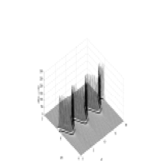
Figure 7: Energy density ( per unit of information) as a function of $\tilde{x}=x/a$ and $t$ for $a/\lambda_{db}=20$

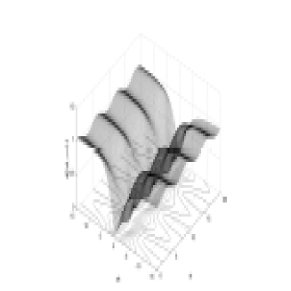
Figure 8: Energy density ( per unit of information) as a function of $\tilde{x}=x/a$ and $t$ for $a/\lambda_{db}=0.5$

The graphs of the general distribution function $dE/dI$ for $2$ values of the parameter $\alpha=a/\lambda_{db}$: $\alpha=20$ (classical regime) and $\alpha=0.5$(quantum regime) are shown in Figures $7$ and $8$. It is seen that in the classical regime the energy expenditure per unit of information is very high in classical regime is centered on the classical trajectory, while in quantum regime this expenditure is ”spread” over the space outside the area occupied by the classical trajectory. This is in full compliance with our previous discussion about the nature of spatial spread of information.

3.2 Further Examples of Quantum Equations as a Consequence of Spatial Information Spread in Respective Classical Equations

As a next step, we apply the same idea to a derivation of the Klein-Gordon equation for a charged relativistic particle of spin $0$ in an electro-magnetic field. To this end we add a small perturbation term (analogous to the above ”dissipative” terms

$$\nu^{q}g^{jk}\frac{\partial}{\partial x^{k}}(\frac{\partial S}{\partial x^{j}}+eA_{j})$$

($\nu^{q}$ is to be determined) to the right hand side of the relativistic Hamilton-Jacobi equation

$$g^{jk}(\frac{\partial S}{\partial x^{j}}+A_{j})(\frac{1}{m}\frac{\partial S}{\partial x^{k}}+\frac{1}{m}eA_{k})=m,$$ (59)

(where we set the speed of light $c=1$) use substitution (40) and get

$$g^{jk}(\frac{\hbar}{i}\frac{\partial\Psi}{\partial x^{j}}+e\Psi A_{j})(\frac{\hbar}{im}\frac{\partial\Psi}{\partial x^{k}}+\frac{e}{m}\Psi A_{k}) =$$

$$m\Psi^{2}+\nu^{q}g^{jk}(\frac{\hbar}{i}\frac{\partial^{2}\Psi}{\partial x^{j}\partial x^{k}}-\frac{\hbar}{i}\frac{\partial\Psi}{\partial x^{j}}\frac{\partial\Psi}{\partial x^{k}}+e\Psi\frac{\partial A_{j}}{\partial x^{k}})$$ (60)

Linearity requirement imposed on this equation determines the value of constant $\nu^{q}$:

$$\nu^{q}=i\frac{\hbar}{m}$$

which is the same as we found before in Eq.(41). Inserting this value back in (3.2) and performing some elementary calculations we arrive at the Klein-Gordon equation for a charged relativistic particle of spin $0$ in an electro-magnetic field:

$$g^{jk}(\frac{\hbar}{i}\frac{\partial}{\partial x^{j}}+eA_{j})(\frac{\hbar}{i}\frac{\partial}{\partial x^{k}}+eA_{k})\Psi=m^{2}\Psi$$ (61)

Since this idea clearly works for particles with zero spin, it is naturally to ask whether it would work for particles with a spin. Here one must be a little bit more ingenious in choosing the appropriate dissipative term to be introduced into the Hamilton-Jacobi equation. If we consider a classical charged particle in the electro-magnetic field it has an additional energy $E_{H}=-\vec{\mu}\centerdot\vec{H}$ due to an interaction of the magnetic moment $\vec{\mu}$ and the magnetic field $\vec{H}$.

In terms of the vector potential $\vec{A}$ this energy is

$$E_{H}=-\vec{\mu}\centerdot(\nabla\times e\vec{A})\equiv div(\vec{\mu}\times e\vec{A})$$ (62)

Experiments demonstrated that the magnetic moment $\vec{\mu_{e}}$ of an electron is proportional to its spin $\vec{s}$:

$$\vec{\mu_{e}}=\frac{\hbar}{m}\vec{s}$$ (63)

It is remarkable that once again ( as in the above cases) the coefficient of proportionality in (63) has the dimension of kinematic viscosity! Its magnitude is twice the magnitude of the $"quasi~{}kinematic~{}viscosity"~{}\nu^{q}$.

If we substitute (63), in (62) we obtain

$$E_{H}=-\frac{\hbar}{m}\nabla\centerdot(\vec{s}\times e\vec{A})$$ (64)

This expression has a structure of the dissipative term introduced earlier in the Hamilton-Jacobi equation (44). Therefore we rewrite this equation with the additional ”dissipative” term (64)

$$\frac{\partial S}{\partial t}+\frac{1}{2m}(\nabla S-e\vec{A})^{2}+e\phi=\nabla\centerdot[\nu^{q}(\nabla S-e\vec{A})-\frac{\hbar}{m}(\vec{s}\times e\vec{A})]$$ (65)

We substitute (40) in (65), use the vector identity

$$\nabla\centerdot(\vec{a}\times\vec{b})\equiv\vec{b}\centerdot curl\vec{b}-\vec{a}\centerdot curl\vec{b}$$

and obtain

$$-i\hbar\Psi\frac{\partial\Psi}{\partial t}+\frac{1}{2m}(\frac{\hbar}{i}\nabla\Psi-e\vec{A}\Psi)^{2}+e\phi\Psi^{2}=$$

$$\Psi^{2}\frac{\hbar}{i}\nu^{q}\nabla\centerdot(\frac{\nabla\Psi}{\Psi})-\Psi^{2}e\frac{\hbar}{m}(\vec{A}\centerdot curl\vec{s}-\vec{s}\centerdot curl\vec{A})$$ (66)

Since the required equation must be linear (which uniquely defines $\nu^{q}$ again as $i\hbar/2m$), and function $\Psi$ now depends on the $z$-component of the spin $\vec{s}$ (that is, it becomes a $2\times 1$ vector-column function) we have to replace vector $\vec{s}$ by the respective ($2\times 2$) matrices $\hat{\vec{s}}$. As a result, we arrive at the Pauli equation:

$$\!i\hbar\frac{\partial\Psi}{\partial t}=\frac{1}{2m}(\frac{\hbar}{i}\nabla-e\vec{A})^{2}\Psi+e\phi\Psi-\frac{e\hbar}{m}(\hat{\vec{s}}\centerdot\vec{H})\Psi$$ (67)

Since the method of information spread introduced into the classical Hamilton-Jacobi equations via the ”effective viscosity” $\nu^{q}$ has turned out to be fruitful so far, we apply it to a simple case of a particle in the gravitational field. The Hamilton-Jacobi equation in this case is

$$g^{jk}S_{;j}S_{;k}-m^{2}=0$$ (68)

where $g^{jk}$ is the metric tensor, $j,k=0,1,2,3$, the $semicolon$ denotes covariant differentiation, and we set $c=1$.

Now we add to the right-hand side of (68) the dissipative term in the form used in the above calculations, that is $\nabla\centerdot(\nu^{q}\nabla S)$. However, this time, instead of the conventional derivatives, we use the covariant derivatives and replace the constant scalar $\nu^{q}$ by a tensor function $\nu^{jk}$. As a result, equation (68) becomes:

$$g^{jk}S_{;j}S_{;k}-m^{2}=(\nu^{jk}S_{;k})_{;j}$$ (69)

By using substitution (40) in (69) and performing some standard calculations we obtain the following

$$-\hbar^{2}g^{jk}\frac{\partial\Psi}{\partial x^{j}}\frac{\partial\Psi}{\partial x^{k}}-m^{2}\Psi^{2}+\frac{\hbar}{i}\nu^{jk}\frac{\partial\Psi}{\partial x^{j}}\frac{\partial\Psi}{\partial x^{k}}-\frac{\hbar}{i}\nu^{jk}_{;j}\Psi\frac{\partial\Psi}{\partial x^{k}}$$

$$-\frac{\hbar}{i}\nu^{jk}\Psi(\frac{\partial^{2}\Psi}{\partial x^{j}\partial x^{k}}+\Gamma_{kj}^{n}\frac{\partial\Psi}{\partial x^{n}})-m^{2}\Psi^{2}=0$$ (70)

where $\Gamma_{jk}^{n}$ is the Ricci tensor. We require this equation to be linear, which uniquely determines the value of the tensor $\nu^{jk}$:

$$\nu^{jk}=i\hbar g^{jk}$$ (71)

Since $g^{jk}_{;j}\equiv 0$ equation (3.2) yields

$$g^{jk}\frac{\partial^{2}\Psi}{\partial x^{j}\partial x^{k}}-\frac{1}{\sqrt{-g}}\frac{\partial}{\partial x^{l}}(\sqrt{-g}g^{nl})\frac{\partial\Psi}{\partial x^{n}}+\kappa^{2}\Psi=0$$ (72)

where $\kappa=m/\hbar$.

As a particular example we consider the centrally symmetric gravitational field with the Schwarzchild metric:

$$g^{jk}=0,j\neq k;~{}~{}~{}g^{00}=\frac{1}{1-r_{g}/r};~{}~{}~{}g^{11}=-(1-\frac{r_{g}}{r});$$

$$g^{22}=-\frac{1}{r^{2}};~{}~{}~{}g^{33}=-(1-\frac{r_{g}}{r});~{}~{}~{}g=|g^{jk}|=-\frac{1}{r^{4}\sin^{2}\theta};~{}~{}~{}r_{g}=2mG$$ (73)

Equation (72) is then

$$\frac{1}{1-r_{g}/r}\frac{\partial^{2}\Psi}{\partial t^{2}}-(1-\frac{r_{g}}{r})\frac{\partial^{2}\Psi}{\partial r^{2}}-\frac{1}{r^{2}sin^{2}\theta}\frac{\partial^{2}\Psi}{\partial\phi^{2}}-$$

$$\frac{1}{r^{2}}\frac{\partial^{2}\Psi}{\partial\theta^{2}}-\frac{2}{r}(1-\frac{3}{2}\frac{r_{g}}{r})\frac{\partial\Psi}{\partial r}-\frac{1}{r^{2}}cot\theta\frac{\partial\Psi}{\partial\theta}+\kappa^{2}\Psi=0$$ (74)

4 Conclusion

Physical phenomena can only be described as either particle-like or wave-like phenomena. Consequently, the critical question arises: Does the complex-valued wave function $\Psi$ represent reality, or is it only an intricate device to deal with something we don’t have a complete knowledge of?

Bohm [17] proposed to remove such indeterminacy and thus to answer the above question by introducing hidden variables into the existing Shr$\mathrm{\ddot{o}}$dinger equation. We treat this problem absolutely differently, first

• by starting from the classical Hamilton-Jacobi equation (without any presumed $a~{}priori$ knowledge of the Shrödinger equation) and arriving at the Shrödinger equation,

  and secondly

• without using any hidden variables, since they are not necessary in such an approach.

Instead, and this is the major idea of our approach, we demonstrate that the above indeterminacy is due to a spread of information over the whole space, with a simultaneous preservation of information, in contradistinction to the classical case where the same information is centered on the classical path occupied by a classical particle.

Such an $information~{}spread$ is described by an information density function which is different from a delta-like function observed in the classical case. In a sense, this resembles a dissipation of temperature in a solid body, but only in a sense, since the total quantity of heat remains unchanged. No wonder that the resulting Shrödinger equation has a form of the diffusion equation, albeit with the imaginary ”time” (which reflects the intrinsic presence of wave features in this phenomenon). More to the point, the above process resembles the transfer of energy from larger to smaller scales in turbulence ( e.g., see Ref. [9]).

As a result, the wave-like quantum mechanics turns out to follow from the particle-like classical mechanics due to the explicit introduction in the latter of a dissipative mechanism responsible for the spread of information. Consequently, the initial precise information about the classical trajectory of a particle is ”spread” (but not lost) over the whole space, which for a simple case of a spinless particle [2], [12] results in a transformation of a classical trajectory into a fractal path with Hausdorff dimension of $2$ .

The idea of quantum mechanics representing a spatial spread of information, implemented (in a general way) in this paper, has not only made it possible to elementary derive the basic quantum-mechanical equations from the continuum equations of classical mechanics, but also seems to be applicable to more complex and intriguing problems, as for example, a relativistic particle in the gravitational field.

Acknowledgments.

Author would like to thank Prof.V.Granik and G.Chapline for the illuminating discussions and constructive criticism.

References

- [1] P.Dirac, The Principles of Quantum Mechanics, Clarendon Press (Oxford),1993
- [2] A. Granik and G.Chapline, Phys.Lett.A 310, 252(2003)
- [3] W.Zurek, Physics Today,Oct.1991
- [4] H.Schlichting, Boundary-Layer Theory, McGraw-Hill Inc.(New York), 1987
- [5] R.Kiehn, Nanometer Vortices(unpublished)
- [6] M.Blazone,P.Jizba, and G.Vitiello, hep-th/0007138
- [7] M.Planck, Eight Lectures on Theoretical Physics, Dover (New York),1998
- [8] G.Chapline et.al., Phil.Mag.B, 81, No.3, 235(2001)
- [9] L.Landau and E.Lifshitz, Fluid Mechanics, Pergamon Press (London), 1959
- [10] E.Schrdinger, Ann.d.Physik,79, 361(1926 )
- [11] R.Feynman and A.Hibbs, Quantum Mechanics and Path Integral,McGraw-Hill (New York),1965
- [12] L.F.Abbott and M.B.Wise, Am. J.Phys 49, 37(1981)
- [13] A.Granik, physics/0309059
- [14] L.Schiff, Quantum Mechanics, McGraw Hill (New York), 1955
- [15] B.Schumacher, in ”Complexity,Entropy, and the Physics of Information”, SFI Studies in the Sciences of Complexity, v.VIII,p.29, Ed.W.Zurek, Addison-wesley, 1990
- [16] J.D.Bekenstein, Phys.Rev. (D23),287(1981)
- [17] D.Bohm, Physical Review (85), 166 (1952); D.Bohm and B.J.Hiley, The Undivided Universe, Routledge (London, New York), 1993
- [18] Letters on Wave Mechanics, Ed.K.Przibram, Philosophical Library (New York), 1967