A Representation of Complex Rational Numbers in Quantum mechanics

Paul Benioff
Physics Division, Argonne National Laboratory
Argonne, IL 60439
e-mail: pbenioff@anl.gov
Abstract

A representation of complex rational numbers in quantum mechanics is described that is not based on logical or physical qubits. It stems from noting that the $0s$ in a product qubit state do not contribute to the number. They serve only as place holders. The representation is based on the distribution of four types of systems on an integer lattice. The four types, labelled as positive real, negative real, positive imaginary, and negative imaginary, are represented by creation and annihilation operators acting on the system vacuum state. Complex rational number states correspond to products of creation operators acting on the vacuum. Various operators, including those for the basic arithmetic operations, are described. The representation used here is based on occupation number states and is given for bosons and fermions.

pacs:
03.67.Lx,03.67.-a,03.65.Ta

I Introduction

Quantum computation and quantum information are subjects of much continuing interest and study. An initial impetus for this work was the realization that as computers became smaller, quantum effects would become more important. Additional interest arose with the discovery of problems Shor ; Grover that could be solved more efficiently on a quantum computer than on a classical machine. Also quantum information, and possibly quantum computation, Lloyd ; Zizzi is of recent interest in addressing problems related to cosmology and quantum gravity.

In all of this work qubits (or qudits for d-dimesional systems) play a basic role. As quantum binary systems the states $|0\rangle,|1\rangle$ of a qubit represent the binary choices in quantum information theory. They also represent the numbers 00 and $1$ as numerical inputs to quantum computers. For $n$ qubits, corresponding product states, such as $|\underline{s}\rangle=\otimes_{j=1}^{n}|s(j)\rangle$ where $s(j)=0\mbox{ or }1,$ represent a specific $n$ qubit information state. Since they also represent numbers,

$$|\underline{s}\rangle\rightarrow\sum_{j=1}^{n}\underline{s}(j)2^{j-1},$$ (1)

they and their linear superpositions are inputs to quantum computers.

It is clear that states of qubits are very important to quantum information theory. However, qubits and their states are not essential to the representation of numbers in quantum mechanics. This is based on the observation that in a state, such as $|10010\rangle$, the $0s$ do not contribute to the numerical value of the state. Instead they function more like place holders. What is important is the distribution of the $1s$ along a discrete lattice. This is shown by Eq. 1 where the value of the number is determined by the distribution of $1s$ at the values of $j$ for which $\underline{s}(j)=1$. The value, $0,$ of $\underline{s}$ at other locations contributes nothing.

This suggests a different type of representation of numbers that does not use qubits. It is based instead on the distributions of $1s$ on an integer lattice. For example the rational number $1001.01$ would be represented here as $1_{3}1_{0}1_{-2}.$ In quantum mechanics these states correspond to position eigenstates of a system on a discrete lattice or path where the positions are labelled by integers. Here the state $|j\rangle$ corresponds to the number $2^{j}$ and $n$ product states, such as $|j_{1},\cdots j_{n}\rangle,$ correspond to $\sum_{k=1}^{n}2^{j_{k}}.$

Here the representation of rational numbers corresponds to those represented by finite strings of binary digits or qubits and not as pairs of such strings. This representation is much easier to use and corresponds to that used in computers. It also is dense in the set of all rational numbers. For quantum states this means that any representation of all nonnegative rational numbers as quantum states would be approximated arbitrarily closely by a finite qubit $|\underline{s}\rangle$ states or states of the form $\otimes_{j\epsilon 1_{s}}|j\rangle$ where $1_{s}=\{j|\underline{s}(j)=1\}.$ In what follows this type of state will be referred to as a rational number state.

This representation is sufficient to describe nonnegative rational numbers in quantum mechanics. There are several ways to extend the treatment to include negative and imaginary rational numbers. These range from one type of system with two internal binary degrees of freedom to four different types of systems. Here an intermediate approach is taken in which two types of systems which have an internal binary degree of freedom are considered. The two internal degrees of freedom correspond to positive and negative and the two types of systems correspond to real and imaginary. An example of such a number in the representation considered here is $r_{+,5}\>r_{-,3}\>i_{-,-2}\>i_{+,4}$

The goal of this paper is to use these ideas to give a quantum mechanical representation of complex rational numbers. Since states with varying numbers of $r+,r-,i+,i-$ systems will be encountered, a Fock space representation is used. Both bosons and fermions will be considered.

The emphasis of this work is to describe a set of quantum states that can be shown to represent complex rational numbers. This requires definitions of the basic arithmetical operations used in the axiomatic definitions of rational numbers and showing that the states have the desired properties.

An additional emphasis is that the state descriptions and properties must be relatively independent of the complex rational numbers that are part of the complex number field $C$ on which the Fock space is based. This means that the description will not be based on a map from quantum states to $C$ that is used to define arithmetic properties of the states. Instead the states and their properties will be described independent of any such map.

It will be seen that the representation used here is more compact with simpler representations of the basic arithmetic operations than those based on qubit states with ”binal” points, e.g., of the form $|\pm 10010.011\rangle$ BenRNQM ; BenRNQMALG . It also extends the representation to complex numbers which was not done in the earlier work. Another (slight) advantage is that linear superpositions of states containing just one system are not entangled in the representation used here. This is not the case for the qubit representation with $0s$ present. An example is the Bell state $(1/\sqrt{2})(|10\rangle\pm|01\rangle).$ Here this state is $(1/\sqrt{2})(|1\rangle\pm|0\rangle),$ which is not entangled. In this state 00 and $1$ are the locations of the $1s$ in the qubit state. This advantage is lost when one considers states with more than one system present.

Another advantage of the representation described here is that it may suggest new physical models for quantum computation that are not qubit based. Whether this is the case or not must await future work.

The use of Fock spaces to describe quantum computation and quantum information is not new. It has been used to describe fermionic Kitaev ; Ozhigov and parafermionic Lidar quantum computation, and quantum logic Gudder ; DChiara . The novelty of the approach taken here is based on a description of complex rational string numbers that is not based on logical or physical qubits. In this sense if differs from Kassman . It also emphasizes basic arithmetic operations instead of quantum logic gates. Also both standard and nonstandard representations of numbers are described. These follow naturally from the occupation number description of quantum states.

Details of the description of the complex rational states are given in the next three sections. The a-c operators are described in Section II. The next section gives properties of these and other operators and their use to describe complex rational states. Section IV describes the arithmetic operations of addition, multiplication, and division to any finite accuracy. The last section summarizes some advantages of the approach used here. Also a possible physical model of standard and nonstandard numbers as pools of four types of Bose Einstein condensates along an integer lattice is briefly discussed.

II Complex Rational States

The representation of complex rational states used here is based on the notion of creating and annihilating two types of systems, at various locations. One type is used for real rational states and the other for imaginary states. For bosons the degrees of freedom associated with each type consist of a binary internal degree, denoted by $+,-$, and a location $j$ on an integer labelled lattice.

The creation operators for bosons are a+,j†,aβˆ’,j†,b+,j†,bβˆ’,j†subscriptsuperscriptπ‘Žβ€ π‘—subscriptsuperscriptπ‘Žβ€ π‘—subscriptsuperscript𝑏†𝑗subscriptsuperscript𝑏†𝑗a^{{\dagger}}_{+,j},a^{{\dagger}}_{-,j},b^{{\dagger}}_{+,j},b^{{\dagger}}_{-,j}. The $a$ operators create and annihilate bosons in states corresponding respectively to positive and negative real rational states. The $b$ operators play the same role for imaginary states. The state $|0\rangle$ is the vacuum state.

In this representation, the states a+,j†​|0⟩,aβˆ’,j†​|0⟩subscriptsuperscriptπ‘Žβ€ π‘—ket0subscriptsuperscriptπ‘Žβ€ π‘—ket0a^{{\dagger}}_{+,j}|0\rangle,a^{{\dagger}}_{-,j}|0\rangle show an a (real) boson in states $+,-$ at site $j$. The states $b^{{\dagger}}_{+,j}|0\rangle,b^{{\dagger}}_{-,j}|0\rangle$ show a b (imaginary) boson in states $+,-$ at site $j$. In the order presented these states correspond to the numbers $2^{j},-2^{j},i2^{j},$ and $-i2^{j}.$

For fermions the creation and annihilation operators have an additional variable $h=0,1,2,\cdots.$ This extra variable is needed to make fermions with the same sign and $j$ value distinguishable. Thus boson states of the form a+,j†​a+,j†​|0⟩subscriptsuperscriptπ‘Žβ€ π‘—subscriptsuperscriptπ‘Žβ€ π‘—ket0a^{{\dagger}}_{+,j}a^{{\dagger}}_{+,j}|0\rangle become a+,h,j†​a+,hβ€²,j†​|0⟩subscriptsuperscriptπ‘Žβ€ β„Žπ‘—subscriptsuperscriptπ‘Žβ€ superscriptβ„Žβ€²π‘—ket0a^{{\dagger}}_{+,h,j}a^{{\dagger}}_{+,h^{\prime},j}|0\rangle where hβ‰ hβ€².β„Žsuperscriptβ„Žβ€²h\neq h^{\prime}. Note that, as far as number properties are concerned, $h$ is a dummy variable in that a+,h,j†​|0⟩subscriptsuperscriptπ‘Žβ€ β„Žπ‘—ket0a^{{\dagger}}_{+,h,j}|0\rangle and a+,hβ€²,j†​|0⟩subscriptsuperscriptπ‘Žβ€ superscriptβ„Žβ€²π‘—ket0a^{{\dagger}}_{+,h^{\prime},j}|0\rangle both represent the same number. However in any physical model it would represent some physical property.

One can also form linear superpositions of these states. Simple boson examples and their equivalences in the usual qubit based binary notation are,

(1/2)​(a+,j†±aβˆ’,j†)​|0⟩=(1/2)​(|1​0Β―j⟩±|βˆ’1​0Β―j⟩)(1/2)​(a+,j†±aβˆ’,k†)​|0⟩=(1/2)​(|1​0Β―j⟩±|βˆ’1​0Β―k⟩)(1/2)​(a+,k†±b+,j†)=(1/2)​(|1​0Β―k⟩±|i​1​0Β―k⟩)(1/2)​(1Β±bβˆ’,j†)​|0⟩=(1/2)​(|0⟩±|βˆ’i​1​0Β―j⟩)(1/2)​(1Β±a+,j†)​|0⟩=(1/2)​(|0⟩±|1​0Β―j⟩).12plus-or-minussubscriptsuperscriptπ‘Žβ€ π‘—subscriptsuperscriptπ‘Žβ€ π‘—ket012plus-or-minusket1superscriptΒ―0𝑗ket1superscriptΒ―0𝑗12plus-or-minussubscriptsuperscriptπ‘Žβ€ π‘—subscriptsuperscriptπ‘Žβ€ π‘˜ket012plus-or-minusket1superscriptΒ―0𝑗ket1superscriptΒ―0π‘˜12plus-or-minussubscriptsuperscriptπ‘Žβ€ π‘˜subscriptsuperscript𝑏†𝑗12plus-or-minusket1superscriptΒ―0π‘˜ket𝑖1superscriptΒ―0π‘˜12plus-or-minus1subscriptsuperscript𝑏†𝑗ket012plus-or-minusket0ket𝑖1superscriptΒ―0𝑗12plus-or-minus1subscriptsuperscriptπ‘Žβ€ π‘—ket012plus-or-minusket0ket1superscriptΒ―0𝑗\begin{array}[]{l}(1/\sqrt{2})(a^{{\dagger}}_{+,j}\pm a^{{\dagger}}_{-,j})|0\rangle=(1/\sqrt{2})(|1\underline{0}^{j}\rangle\pm|-1\underline{0}^{j}\rangle)\\ (1/\sqrt{2})(a^{{\dagger}}_{+,j}\pm a^{{\dagger}}_{-,k})|0\rangle=(1/\sqrt{2})(|1\underline{0}^{j}\rangle\pm|-1\underline{0}^{k}\rangle)\\ (1/\sqrt{2})(a^{{\dagger}}_{+,k}\pm b^{{\dagger}}_{+,j})=(1/\sqrt{2})(|1\underline{0}^{k}\rangle\pm|i1\underline{0}^{k}\rangle)\\ (1/\sqrt{2})(1\pm b^{{\dagger}}_{-,j})|0\rangle=(1/\sqrt{2})(|0\rangle\pm|-i1\underline{0}^{j}\rangle)\\ (1/\sqrt{2})(1\pm a^{{\dagger}}_{+,j})|0\rangle=(1/\sqrt{2})(|0\rangle\pm|1\underline{0}^{j}\rangle).\end{array} (2)

Here $\underline{0}^{j}$ represents a string of $j$ $0s.$

These states show one advantage of the representation used here in that those on the left are valid for any value of $j$ or $k$. The usual binary representations on the right are valid only for $j,k\geq 0.$ Note also that $-$ and $i$ inside the qubit states denote the type and sign of the number. They are not phase factors multiplying the states.

III Occupation Number States

The first step in representing states as products of creation operators acting on $|0\rangle$ is to give the commutation relations. Let $c^{{\dagger}}_{j},\hat{c}^{{\dagger}}_{j},c_{j},$ and $\hat{c}_{j}$ be variable a-c operators where $c^{{\dagger}}$ and $\hat{c}^{{\dagger}}$ can take any one of the four values a+†,aβˆ’β€ ,b+†,bβˆ’β€ .subscriptsuperscriptπ‘Žβ€ subscriptsuperscriptπ‘Žβ€ subscriptsuperscript𝑏†subscriptsuperscript𝑏†a^{{\dagger}}_{+},a^{{\dagger}}_{-},b^{{\dagger}}_{+},b^{{\dagger}}_{-}. Using these the boson commutation relations can be given as

[cj,ck†]=Ξ΄j,k[cj†,c^k†]=[cj,c^k]=0.formulae-sequencesubscript𝑐𝑗subscriptsuperscriptπ‘β€ π‘˜subscriptπ›Ώπ‘—π‘˜subscriptsuperscript𝑐†𝑗subscriptsuperscript^π‘β€ π‘˜subscript𝑐𝑗subscript^π‘π‘˜0[c_{j},c^{{\dagger}}_{k}]=\delta_{j,k}\hskip 28.45274pt[c^{{\dagger}}_{j},\hat{c}^{{\dagger}}_{k}]=[c_{j},\hat{c}_{k}]=0. (3)

The first equation stands for four equations as $c^{{\dagger}}$ has any one of four values. Each of the next two equations stands for $16$ equations as $c^{{\dagger}}$ and $\hat{c}^{{\dagger}}$ each have any one of four values.

For fermions the anticommutation relations are given by

{cg,j,ch,k†}=Ξ΄j,k​δg,h{cg,j†,c^h,k†}={cg,j,c^h,k}=0formulae-sequencesubscript𝑐𝑔𝑗subscriptsuperscriptπ‘β€ β„Žπ‘˜subscriptπ›Ώπ‘—π‘˜subscriptπ›Ώπ‘”β„Žsubscriptsuperscript𝑐†𝑔𝑗subscriptsuperscript^π‘β€ β„Žπ‘˜subscript𝑐𝑔𝑗subscript^π‘β„Žπ‘˜0\{c_{g,j},c^{{\dagger}}_{h,k}\}=\delta_{j,k}\delta_{g,h}\hskip 14.22636pt\{c^{{\dagger}}_{g,j},\hat{c}^{{\dagger}}_{h,k}\}=\{c_{g,j},\hat{c}_{h,k}\}=0 (4)

where $\{c,d\}=cd+dc.$ There are two sets of these relations, one for $c^{{\dagger}}$ and $\hat{c}^{{\dagger}}$ each having the values a+†,aβˆ’β€ subscriptsuperscriptπ‘Žβ€ subscriptsuperscriptπ‘Žβ€ a^{{\dagger}}_{+},a^{{\dagger}}_{-} and the other for $c^{{\dagger}}$ and $\hat{c}^{{\dagger}}$ with the values $b^{{\dagger}}_{+}$ or bβˆ’β€ .subscriptsuperscript𝑏†b^{{\dagger}}_{-}. Note that because the $a$ and $b$ systems are two different types of fermions, commutation relations hold between their operators, as in [a+,g,j†,b+,h,k†]=0,subscriptsuperscriptπ‘Žβ€ π‘”π‘—subscriptsuperscriptπ‘β€ β„Žπ‘˜0[a^{{\dagger}}_{+,g,j},b^{{\dagger}}_{+,h,k}]=0, etc..

A complete basis set of states can be defined in terms of occupation numbers of the various boson or fermion states. A general basis can be defined as follows: Let $n_{r},m_{r},n_{i},m_{i}$ be any four functions that map the set of all integers to the nonnegative integers. Each function has the value 00 except possibly on finite sets of integers. Let $s,s^{\prime},t,t^{\prime}$ be the four finite sets of integers which are the nonzero domains, respectively, of the four functions. Thus nr,jβ‰ 0[=0]subscriptπ‘›π‘Ÿπ‘—annotated0delimited-[]absent0n_{r,j}\neq 0[=0] if $j\epsilon s[j\mbox{ not in }s],$ mr,jβ‰ 0[=0]subscriptπ‘šπ‘Ÿπ‘—annotated0delimited-[]absent0m_{r,j}\neq 0[=0] if $j\epsilon s^{\prime}[j\mbox{ not in }s^{\prime}],$ etc..

Let $\bigcup s,t$ be the set of all integers in one or more of the four sets. Then a general boson occupation number state has the form

$$|n_{r},m_{r},n_{i},m_{i}\rangle=\prod_{j\epsilon\cup s,t}|n_{r,j},m_{r,j}n_{i,j}m_{i,j}\rangle$$ (5)

where $|n_{r,j},m_{r,j}n_{i,j}m_{i,j}\rangle$ the occupation number state for site $j$ is given by

|nr,j,mr,j​ni,j​mi,j⟩=1N​(n,m,r,i,j)Γ—(a+,j†)nr,j​(aβˆ’,j†)mr,j​(b+,j†)ni,j​(bβˆ’,j†)mi,j​|0⟩.ketsubscriptπ‘›π‘Ÿπ‘—subscriptπ‘šπ‘Ÿπ‘—subscript𝑛𝑖𝑗subscriptπ‘šπ‘–π‘—1π‘π‘›π‘šπ‘Ÿπ‘–π‘—absentsuperscriptsubscriptsuperscriptπ‘Žβ€ π‘—subscriptπ‘›π‘Ÿπ‘—superscriptsubscriptsuperscriptπ‘Žβ€ π‘—subscriptπ‘šπ‘Ÿπ‘—superscriptsubscriptsuperscript𝑏†𝑗subscript𝑛𝑖𝑗superscriptsubscriptsuperscript𝑏†𝑗subscriptπ‘šπ‘–π‘—ket0\begin{array}[]{l}|n_{r,j},m_{r,j}n_{i,j}m_{i,j}\rangle=\frac{1}{N(n,m,r,i,j)}\\ \hskip 28.45274pt\times(a^{{\dagger}}_{+,j})^{n_{r,j}}(a^{{\dagger}}_{-,j})^{m_{r,j}}(b^{{\dagger}}_{+,j})^{n_{i,j}}(b^{{\dagger}}_{-,j})^{m_{i,j}}|0\rangle.\end{array} (6)

The normalization factor $N(n,m,r,i,j)=(n_{r,j}!m_{r,j}!n_{i,j}!m_{i,j}!)^{1/2}.$ Note that the product $\prod_{j\epsilon\cup s,t}$ denotes a product of creation operators, and not a product of states.

The interpretation of these states is that they are the boson equivalent of nonstandard representations of complex rational numbers as distinct from standard representations. (This use of standard and nonstandard is completely different from standard and nonstandard numbers described in mathematical logic Chang .) Such nonstandard states occur often in arithmetic operations and will be encountered later on. They correspond to columns of binary numbers where each number in the column is any one of the four types, positive real, negative real, positive imaginary, and negative imaginary. In a boson representation individual systems, are not distinguishable. The only measurable properties are the number of systems of each type $+1,-1,+i,-i$ in the single digit column at each site $j.$

An example would be a computation in which one computes the value of the integral $\int_{a}^{b}f(x)dx$ of a complex valued function $f$ by computing in parallel, or by a quantum computation, values of $f(x_{h})$ for $h=1,2,\cdots,m$ and then combining the $m$ results to get the final answer. The table, or matrix, of $m$ results before combination is represented here by a state $|n_{r},m_{r},n_{i},m_{i}\rangle$ where $n_{r,j},m_{r,j}n_{i,j},m_{i,j}$ give the number of $+1^{\prime}s$, $-1^{\prime}s,$ $+i^{\prime}s$, and $-i^{\prime}s$ in the column at site $j.$ This is a nonstandard representation because it is numerically equal to the final result which is a standard representation consisting of one real and one imaginary rational string number, often represented as a pair, $u,iv$.

The equivalent fermionic representation for the state $|n_{r},m_{r},n_{i},m_{i}\rangle$ is based on a fixed ordering of the a-c operators. In this case the product (a+,j†)nr,jsuperscriptsubscriptsuperscriptπ‘Žβ€ π‘—subscriptπ‘›π‘Ÿπ‘—(a^{{\dagger}}_{+,j})^{n_{r,j}} becomes a+1,j†​⋯​a+h,j†​⋯​a+nr,j,j†subscriptsuperscriptπ‘Žβ€ 1𝑗⋯subscriptsuperscriptπ‘Žβ€ β„Žπ‘—β‹―subscriptsuperscriptπ‘Žβ€ subscriptπ‘›π‘Ÿπ‘—π‘—a^{{\dagger}}_{+1,j}\cdots a^{{\dagger}}_{+h,j}\cdots a^{{\dagger}}_{+n_{r,j},j} with similar replacements for (aβˆ’,j†)mr,j,(b+,j†)ni,j,(bβˆ’,j†)mi,j.superscriptsubscriptsuperscriptπ‘Žβ€ π‘—subscriptπ‘šπ‘Ÿπ‘—superscriptsubscriptsuperscript𝑏†𝑗subscript𝑛𝑖𝑗superscriptsubscriptsuperscript𝑏†𝑗subscriptπ‘šπ‘–π‘—(a^{{\dagger}}_{-,j})^{m_{r,j}},(b^{{\dagger}}_{+,j})^{n_{i,j}},(b^{{\dagger}}_{-,j})^{m_{i,j}}. Each component state $|n_{r,j},m_{r,j},n_{i,j},m_{i,j}\rangle$ in Eq. 6 is given by

|nr,j,mr,j,ni,j,mi,j⟩=a+nr,j,j†​⋯​a+1,j†​aβˆ’mr,j,j†​⋯aβˆ’1,j†​b+ni,j,j†​⋯​b+1,j†​bβˆ’mi,j,j†​⋯​bβˆ’1,j†​|0⟩ketsubscriptπ‘›π‘Ÿπ‘—subscriptπ‘šπ‘Ÿπ‘—subscript𝑛𝑖𝑗subscriptπ‘šπ‘–π‘—subscriptsuperscriptπ‘Žβ€ subscriptπ‘›π‘Ÿπ‘—π‘—β‹―subscriptsuperscriptπ‘Žβ€ 1𝑗subscriptsuperscriptπ‘Žβ€ subscriptπ‘šπ‘Ÿπ‘—π‘—β‹―subscriptsuperscriptπ‘Žβ€ 1𝑗subscriptsuperscript𝑏†subscript𝑛𝑖𝑗𝑗⋯subscriptsuperscript𝑏†1𝑗subscriptsuperscript𝑏†subscriptπ‘šπ‘–π‘—π‘—β‹―subscriptsuperscript𝑏†1𝑗ket0\begin{array}[]{c}|n_{r,j},m_{r,j},n_{i,j},m_{i,j}\rangle=a^{{\dagger}}_{+n_{r,j},j}\cdots a^{{\dagger}}_{+1,j}a^{{\dagger}}_{-m_{r,j},j}\cdots\\ a^{{\dagger}}_{-1,j}b^{{\dagger}}_{+n_{i,j},j}\cdots b^{{\dagger}}_{+1,j}b^{{\dagger}}_{-m_{i,j},j}\cdots b^{{\dagger}}_{-1,j}|0\rangle\end{array} (7)

The final state is given by an ordered product over the $j$ value,

$$|n_{r},m_{r},n_{i},m_{i}\rangle=\prod_{j\epsilon\cup s,t}J|n_{r,j},m_{r,j}n_{i,j}m_{i,j}\rangle.$$ (8)

Here $J$ denotes a $j$ ordered product where factors with larger values of $j$ are to the right of factors with smaller $j$ values. The choice of ordering, such as that used here in which the ordering of the $j$ values is the opposite of that for the $h$ values which increase to the left as in Eq. 7, is arbitrary. However, it must remain fixed throughout.

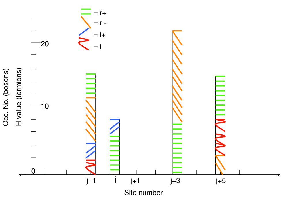
An example of a nonstandard representation is illustrated in Figure 1 for both bosons and fermions. The integer values of $j$ are shown on the abcissa. The ordinate shows the boson occupation numbers for each type of system. Fermions are represented as two types of systems each with two internal states $(+,-)$ on a two dimensional lattice with $j$ any integer and $h$ any nonnegative integer. The ordinate shows the range of $h$ values from 00 to $n_{r,j},m_{r,j},n_{i,j},m_{i,j}$ for each of the four types.

Refer to caption
Figure 1: Example of a nonstandard complex rational state for bosons and fermions for $4$ occupied $j$ values. At each site $j$ the vertical bar shows the occupation numbers (bosons) or extent of $h$ values (fermions) with different colors and line slopes showing each of the four types of systems. For instance the bar at site $j-1$ shows $13\;r+,$ $11\;r-,$ $4\;i+,$ and $2\;i-$ systems and the bar at site $j$ shows $5\;r+$ and $8\;i+$ bosons. For fermions the ordinate labels the ranges of the $h$ values for each type.

The above shows the importance of nonstandard representations, especially in cases where a large amount of data or numbers is generated which must be combined into a single numerically equivalent complex rational number. This requires definition of standard complex rational number states and of properties to be satisfied by any conversion process.

For bosons a standard complex rational state has the form of Eq. 6 where one of the functions $n_{r},m_{r}$ and one of $n_{i},m_{i}$ has the constant value $1$ on their nonzero domains. The other two functions are 00. The four possibilities are

|1Β―s,0,1Β―t,0⟩=(a+†)s​(b+†)t​|0⟩|1Β―s,0,0,1Β―tβ€²βŸ©=(a+†)s​(bβˆ’β€ )t′​|0⟩|0,1Β―sβ€²,1Β―t,0⟩=(aβˆ’β€ )s′​(b+†)t​|0⟩|0,1Β―sβ€²,0,1Β―tβ€²βŸ©=(aβˆ’β€ )s′​(bβˆ’β€ )t′​|0⟩.ketsubscriptΒ―1𝑠0subscriptΒ―1𝑑0superscriptsubscriptsuperscriptπ‘Žβ€ π‘ superscriptsubscriptsuperscript𝑏†𝑑ket0ketsubscriptΒ―1𝑠00subscriptΒ―1superscript𝑑′superscriptsubscriptsuperscriptπ‘Žβ€ π‘ superscriptsubscriptsuperscript𝑏†superscript𝑑′ket0ket0subscriptΒ―1superscript𝑠′subscriptΒ―1𝑑0superscriptsubscriptsuperscriptπ‘Žβ€ superscript𝑠′superscriptsubscriptsuperscript𝑏†𝑑ket0ket0subscriptΒ―1superscript𝑠′0subscriptΒ―1superscript𝑑′superscriptsubscriptsuperscriptπ‘Žβ€ superscript𝑠′superscriptsubscriptsuperscript𝑏†superscript𝑑′ket0\begin{array}[]{c}|\underline{1}_{s},0,\underline{1}_{t},0\rangle=(a^{{\dagger}}_{+})^{s}(b^{{\dagger}}_{+})^{t}|0\rangle\\ |\underline{1}_{s},0,0,\underline{1}_{t^{\prime}}\rangle=(a^{{\dagger}}_{+})^{s}(b^{{\dagger}}_{-})^{t^{\prime}}|0\rangle\\ |0,\underline{1}_{s^{\prime}},\underline{1}_{t},0\rangle=(a^{{\dagger}}_{-})^{s^{\prime}}(b^{{\dagger}}_{+})^{t}|0\rangle\\ |0,\underline{1}_{s^{\prime}},0,\underline{1}_{t^{\prime}}\rangle=(a^{{\dagger}}_{-})^{s^{\prime}}(b^{{\dagger}}_{-})^{t^{\prime}}|0\rangle.\end{array} (9)

Here (a+†)s=∏j​ϡ​sa+,j†superscriptsubscriptsuperscriptπ‘Žβ€ π‘ subscriptproduct𝑗italic-ϡ𝑠subscriptsuperscriptπ‘Žβ€ π‘—(a^{{\dagger}}_{+})^{s}=\prod_{j\epsilon s}a^{{\dagger}}_{+,j} and $\underline{1}_{s}$ denotes the constant $1$ function on $s$, etc. Pure real or imaginary standard rational states are included if $t,\;t^{\prime}$ or $s,\;s^{\prime}$ are empty. If $s,\;s^{\prime},\;t,\;t^{\prime}$ are all empty one has the vacuum state $|0\rangle.$ Note that Eq. 9 also is valid for fermions with the replacements

(aα†)sβ†’aΞ±,1,j1†​aΞ±,1,j2†​⋯​aΞ±,1,j|s|†(bβ†)tβ†’bΞ²,1,k1†​bΞ²,1,k2†​⋯​bΞ²,1,k|t|†.β†’superscriptsubscriptsuperscriptπ‘Žβ€ π›Όπ‘ subscriptsuperscriptπ‘Žβ€ π›Ό1subscript𝑗1subscriptsuperscriptπ‘Žβ€ π›Ό1subscript𝑗2β‹―subscriptsuperscriptπ‘Žβ€ π›Ό1subscript𝑗𝑠→superscriptsubscriptsuperscript𝑏†𝛽𝑑subscriptsuperscript𝑏†𝛽1subscriptπ‘˜1subscriptsuperscript𝑏†𝛽1subscriptπ‘˜2β‹―subscriptsuperscript𝑏†𝛽1subscriptπ‘˜π‘‘\begin{array}[]{l}(a^{{\dagger}}_{\alpha})^{s}\rightarrow a^{{\dagger}}_{\alpha,1,j_{1}}a^{{\dagger}}_{\alpha,1,j_{2}}\cdots a^{{\dagger}}_{\alpha,1,j_{|s|}}\\ (b^{{\dagger}}_{\beta})^{t}\rightarrow b^{{\dagger}}_{\beta,1,k_{1}}b^{{\dagger}}_{\beta,1,k_{2}}\cdots b^{{\dagger}}_{\beta,1,k_{|t|}}.\end{array} (10)

Here $\alpha=+,-$, $\beta=+,-$, and $s=\{j_{1},j_{2},\cdots,j_{|s|}\},\;t=\{k_{1},k_{2},\cdots,k_{|t|}\}$. Also $j_{1}<j_{2}<\cdots<j_{|s|},\;k_{1}<k_{2}<\cdots<k_{|t|},$ and $|s|,|t|$ denote the number of integers in $s,t.$

Standard states are quite important. All theoretical predictions as computational outputs, and numerical experimental results are represented by standard real rational states. Nonstandard representations occur during the computation process and in any situation where a large amount of numbers is to be combined. Also qubit states correspond to standard representations only.

This shows that it is important to describe the numerical relations between nonstandard representations and standard representations and to define numerical equality between states. To this end let

$$|n_{r},m_{r},n_{i},m_{i}\rangle=_{N}|n^{\prime}_{r},m^{\prime}_{r},n^{\prime}_{i},m^{\prime}_{i}\rangle$$ (11)

be the statement of $N$ equality between the two indicated states. This statement is satisfied if two basic equivalences are satisfied. For bosons the two $N$ equivalences are

a+,j†​aβˆ’,j†=N1~;b+,j†​bβˆ’,j†=N1~formulae-sequencesubscript𝑁subscriptsuperscriptπ‘Žβ€ π‘—subscriptsuperscriptπ‘Žβ€ π‘—~1subscript𝑁subscriptsuperscript𝑏†𝑗subscriptsuperscript𝑏†𝑗~1a^{{\dagger}}_{+,j}a^{{\dagger}}_{-,j}=_{N}\tilde{1};\;\;\;\;b^{{\dagger}}_{+,j}b^{{\dagger}}_{-,j}=_{N}\tilde{1} (12)

and

aΞ±,j†​aΞ±,j†=NaΞ±,j+1†aΞ±,j​aΞ±,j=NaΞ±,j+1bΞ²,j†​bΞ²,j†=NbΞ²,j+1†bΞ²,j​bΞ²,j=NbΞ²,j+1.formulae-sequencesubscript𝑁subscriptsuperscriptπ‘Žβ€ π›Όπ‘—subscriptsuperscriptπ‘Žβ€ π›Όπ‘—subscriptsuperscriptπ‘Žβ€ π›Όπ‘—1subscript𝑁subscriptπ‘Žπ›Όπ‘—subscriptπ‘Žπ›Όπ‘—subscriptπ‘Žπ›Όπ‘—1formulae-sequencesubscript𝑁subscriptsuperscript𝑏†𝛽𝑗subscriptsuperscript𝑏†𝛽𝑗subscriptsuperscript𝑏†𝛽𝑗1subscript𝑁subscript𝑏𝛽𝑗subscript𝑏𝛽𝑗subscript𝑏𝛽𝑗1\begin{array}[]{l}a^{{\dagger}}_{\alpha,j}a^{{\dagger}}_{\alpha,j}=_{N}a^{{\dagger}}_{\alpha,j+1}\;\;\;\;a_{\alpha,j}a_{\alpha,j}=_{N}a_{\alpha,j+1}\\ b^{{\dagger}}_{\beta,j}b^{{\dagger}}_{\beta,j}=_{N}b^{{\dagger}}_{\beta,j+1}\;\;\;\;b_{\beta,j}b_{\beta,j}=_{N}b_{\beta,j+1}.\end{array} (13)

The first pair of equations says that any state that has one or more $+$ and $-$ systems of either the $r$ or $i$ type at a site $j$ is numerically equivalent to the state with one less $+$ and $-$ system at the site $j$ of either type. This is the expression here of $2^{j}-2^{j}=i2^{j}-i2^{j}=0.$ The second set of two pairs, Eq. 13, says that any state with two systems of the same type and in the same internal state at site $j$, is numerically equivalent to a state without these systems but with one system of the same type and internal state at site $j+1.$ This corresponds to $2^{j}+2^{j}=2^{j+1}$ or $i2^{j}+i2^{j}=i2^{j+1}.$

From these relations one sees that any process whose iteration preserves $N$ equality according to Eqs. 12 and 13 can be used to determine if Eq. 11 is valid for two different states. For example if

$$|n_{r},m_{r},n_{i},m_{i}\rangle=a_{+,j}a_{-,j}|n^{\prime}_{r},m^{\prime}_{r},n^{\prime}_{i},m^{\prime}_{i}\rangle$$ (14)

or

$$|n_{r},m_{r},n_{i},m_{i}\rangle=b^{{\dagger}}_{+,j+1}b_{+,j}b_{+,j}|n^{\prime}_{r},m^{\prime}_{r},n^{\prime}_{i},m^{\prime}_{i}\rangle,$$ (15)

then Eq. 11 is satisfied.

For fermions the corresponding $N$ equivalences are

a+,j,h†​aβˆ’,j,h′†=N1~;b+,j,h†​bβˆ’,j,h′†=N1~formulae-sequencesubscript𝑁subscriptsuperscriptπ‘Žβ€ π‘—β„Žsubscriptsuperscriptπ‘Žβ€ π‘—superscriptβ„Žβ€²~1subscript𝑁subscriptsuperscriptπ‘β€ π‘—β„Žsubscriptsuperscript𝑏†𝑗superscriptβ„Žβ€²~1a^{{\dagger}}_{+,j,h}a^{{\dagger}}_{-,j,h^{\prime}}=_{N}\tilde{1};\;\;\;\;b^{{\dagger}}_{+,j,h}b^{{\dagger}}_{-,j,h^{\prime}}=_{N}\tilde{1} (16)

and

$$\begin{array}[]{l}a^{{\dagger}}_{\alpha,h,j}a^{{\dagger}}_{\alpha,h^{\prime},j}=_{N}a^{{\dagger}}_{\alpha,h^{\prime\prime},j+1}\;\;\;\;a_{\alpha,h,j}a_{\alpha,h^{\prime},j}=_{N}a_{\alpha,h,^{\prime\prime},j+1}\\ b^{{\dagger}}_{\beta,h,j}b^{{\dagger}}_{\beta,h^{\prime},j}=_{N}b^{{\dagger}}_{\beta,h^{\prime\prime},j+1}\;\;\;\;b_{\beta,h,j}b_{\beta,h^{\prime},j}=_{N}b_{\beta,h^{\prime\prime},j+1}.\end{array}$$ (17)

In Eq. 17 hβ‰ hβ€².β„Žsuperscriptβ„Žβ€²h\neq h^{\prime}. Otherwise the values of $h,h^{\prime},h^{\prime\prime}\geq 1$ are arbitrary except that removal of fermions is restricted to occupied $h$ values and addition is restricted to unoccupied values. To avoid poking holes in the $h$ columns at each site $j,$ Fig. 1, it is useful to restrict system removal to the maximum occupied h value and system addition to the nearest unoccupied $h$ site. Numerically it does not matter where, in the $h$ direction, the fermions are added or removed.

These equations have a meaning similar that that for the corresponding boson equations. Eq. 16 says that any state given by Eqs. 7 and 8 is $N$ equal to a state with one a+†subscriptsuperscriptπ‘Žβ€ a^{{\dagger}}_{+} and one aβˆ’β€ subscriptsuperscriptπ‘Žβ€ a^{{\dagger}}_{-} fermion removed from site $j$ i.e. $n_{r,j}\rightarrow n_{r,j}-1$ and $m_{r,j}\rightarrow m_{r,j}-1.$ A similar situation holds for removal of one $b^{{\dagger}}_{+}$ and one bβˆ’β€ subscriptsuperscript𝑏†b^{{\dagger}}_{-} fermion from site $j.$ Eq. 17 says that a state with two a+†subscriptsuperscriptπ‘Žβ€ a^{{\dagger}}_{+} or two aβˆ’β€ subscriptsuperscriptπ‘Žβ€ a^{{\dagger}}_{-} fermions removed from site $j$ is $N$ equal to a state with one a+†subscriptsuperscriptπ‘Žβ€ a^{{\dagger}}_{+} or aβˆ’β€ subscriptsuperscriptπ‘Žβ€ a^{{\dagger}}_{-} fermion added to site $j+1.$ A similar situation holds for the $b^{{\dagger}}_{+}$ or bβˆ’β€ subscriptsuperscript𝑏†b^{{\dagger}}_{-} fermions.

Corresponding to Eq. 14 one has the following: Let $|n_{r},m_{r},n_{i},m_{i}\rangle$ and $|n^{\prime}_{r},m^{\prime}_{r},n^{\prime}_{i},m^{\prime}_{i}\rangle$ be such that

$$|n_{r},m_{r},n_{i},m_{i}\rangle=R_{a,+,j}R_{a,-,j}|n^{\prime}_{r}m^{\prime}_{r}n^{\prime}_{i}m^{\prime}_{i}\rangle$$ (18)

is satisfied where

Ra,+,j=βˆ‘ha+,h+1,j​a+,h+1,j†​a+,h,jRa,βˆ’,j=βˆ‘haβˆ’,h+1,j​aβˆ’,h+1,j†​aβˆ’,h,j,subscriptπ‘…π‘Žπ‘—subscriptβ„Žsubscriptπ‘Žβ„Ž1𝑗subscriptsuperscriptπ‘Žβ€ β„Ž1𝑗subscriptπ‘Žβ„Žπ‘—subscriptπ‘…π‘Žπ‘—subscriptβ„Žsubscriptπ‘Žβ„Ž1𝑗subscriptsuperscriptπ‘Žβ€ β„Ž1𝑗subscriptπ‘Žβ„Žπ‘—\begin{array}[]{l}R_{a,+,j}=\sum_{h}a_{+,h+1,j}a^{{\dagger}}_{+,h+1,j}a_{+,h,j}\\ R_{a,-,j}=\sum_{h}a_{-,h+1,j}a^{{\dagger}}_{-,h+1,j}a_{-,h,j},\end{array} (19)

then Eq. 11 is satisfied. A similar statement holds if $b$ replaces $a$ in the above. The presence of the factors a+,h+1,j​a+,h+1,j†subscriptπ‘Žβ„Ž1𝑗subscriptsuperscriptπ‘Žβ€ β„Ž1𝑗a_{+,h+1,j}a^{{\dagger}}_{+,h+1,j} and aβˆ’,h+1,j​aβˆ’,h+1,j†subscriptπ‘Žβ„Ž1𝑗subscriptsuperscriptπ‘Žβ€ β„Ž1𝑗a_{-,h+1,j}a^{{\dagger}}_{-,h+1,j} in Eq. 19 is to ensure that the a+†subscriptsuperscriptπ‘Žβ€ a^{{\dagger}}_{+} and aβˆ’β€ subscriptsuperscriptπ‘Žβ€ a^{{\dagger}}_{-} operators with the maximum $h$ values are deleted.

Corresponding to Eq. 15 one has that if $|n_{r},m_{r},n_{i},m_{i}\rangle$ and $|n^{\prime}_{r},m^{\prime}_{r},n^{\prime}_{i},m^{\prime}_{i}\rangle$ satisfy

$$|n_{r},m_{r},n_{i},m_{i}\rangle=_{\pm}S_{a,+,j}|n^{\prime}_{r},m^{\prime}_{r},n^{\prime}_{i},m^{\prime}_{i}\rangle$$ (20)

where

Sa,+,j=βˆ‘hβ€²a+,hβ€²+1,j​a+,hβ€²+1,j†​a+,hβ€²,jβ€ Γ—βˆ‘ha+,h+1,ja+,h+1,j†a+,h,ja+,h,j,\begin{array}[]{l}S_{a,+,j}=\sum_{h^{\prime}}a_{+,h^{\prime}+1,j}a^{{\dagger}}_{+,h^{\prime}+1,j}a^{{\dagger}}_{+,h^{\prime},j}\\ \hskip 8.5359pt\times\sum_{h}a_{+,h+1,j}a^{{\dagger}}_{+,h+1,j}a_{+,h,j}a_{+,h,j},\end{array} (21)

then Eq. 11 is satisfied. There are three other equations one each for $S_{a,-,j},S_{b,+,j}$ and $S_{b,-,j}.$

The expression $=_{\pm}$ denotes equality up to a possible sign change. This can occur because the $S$ operators are products of an odd number of a-c operators. If one wants to implement these state reduction steps dynamically with operators that preserve fermion (or boson) number, then a pool of additional fermions (or bosons) must be available to serve as a source or sink of systems. This is not included here because the emphasis is on defining complex rational states and their arithmetic properties.

It is worth noting that Eqs. 14, 15, 18, and 20 can be regarded as axiomatic definitions of $=_{N}$ with no reference to their numerical meaning in terms of powers of $2$. The use of numbers in their description is included as an aid to the reader. It plays no role in their definition.Later on a map from the complex states to $C$ will be defined that shows that these properties of $=_{N}$ are consistent with the map.

Reduction of a nonstandard representation to a standard one proceeds by iteration of steps based on the above equivalences. At some point the process stops when one ends up with a state with at most one system of the $a$ or $b$ type at each site $j$. This is the case for both bosons and fermions. The possible options for each $j$ can be expressed as

$$\begin{array}[]{l}|n_{r,j},m_{r,j},n_{i,j},m_{i,j}\rangle=\left\{\begin{array}[]{l}|1,0,0,1\rangle\\ |1,0,1,0\rangle\\ |0,1,0,1\rangle\\ |0,1,1,0\rangle\end{array}\mbox{ or }\left\{\begin{array}[]{l}|0,0,0,1\rangle\\ |0,0,1,0\rangle\\ |1,0,0,0\rangle\\ |0,1,0,0\rangle\end{array}\right.\right.\\ \mbox{}\\ \hskip 85.35826pt\mbox{ or }|0,0,0,0\rangle.\end{array}$$ (22)

An example of such a state for several $j$ is $|1_{+,3}i_{+,3}1_{-,2}i_{-,4}1_{-,-6}\rangle.$ This state corresponds to the number $2^{3}-2^{2}-2^{-6}+i(2^{3}-2^{4}).$

Conversion of a state in this form into a standard state requires first determining the signs of the $a$ and $b$ systems occupying the sites with the largest $j$ values. This determines the signs separately for the real and imaginary components of the standard representation. In the example given above the real component is $+$ as $3>2,-6$ and the imaginary component is $-$ as $4>3.$

Conversion of all a-c operators into the same kind, as shown in Eq. 9, is based on four relations obtained by iteration of Eq. 13 and use of Eq. 12. For $k<j$ and for bosons they are

a+,j†​aβˆ’,k†=Na+,jβˆ’1†​⋯​a+,k†aβˆ’,j†​a+,k†=Naβˆ’,jβˆ’1†​⋯​aβˆ’,k†b+,j†​bβˆ’,k†=Nb+,jβˆ’1†​⋯​b+,k†bβˆ’,j†​b+,k†=Nbβˆ’,jβˆ’1†​⋯​bβˆ’,k†.subscript𝑁subscriptsuperscriptπ‘Žβ€ π‘—subscriptsuperscriptπ‘Žβ€ π‘˜subscriptsuperscriptπ‘Žβ€ π‘—1β‹―subscriptsuperscriptπ‘Žβ€ π‘˜subscript𝑁subscriptsuperscriptπ‘Žβ€ π‘—subscriptsuperscriptπ‘Žβ€ π‘˜subscriptsuperscriptπ‘Žβ€ π‘—1β‹―subscriptsuperscriptπ‘Žβ€ π‘˜subscript𝑁subscriptsuperscript𝑏†𝑗subscriptsuperscriptπ‘β€ π‘˜subscriptsuperscript𝑏†𝑗1β‹―subscriptsuperscriptπ‘β€ π‘˜subscript𝑁subscriptsuperscript𝑏†𝑗subscriptsuperscriptπ‘β€ π‘˜subscriptsuperscript𝑏†𝑗1β‹―subscriptsuperscriptπ‘β€ π‘˜\begin{array}[]{l}a^{{\dagger}}_{+,j}a^{{\dagger}}_{-,k}=_{N}a^{{\dagger}}_{+,j-1}\cdots a^{{\dagger}}_{+,k}\\ a^{{\dagger}}_{-,j}a^{{\dagger}}_{+,k}=_{N}a^{{\dagger}}_{-,j-1}\cdots a^{{\dagger}}_{-,k}\\ b^{{\dagger}}_{+,j}b^{{\dagger}}_{-,k}=_{N}b^{{\dagger}}_{+,j-1}\cdots b^{{\dagger}}_{+,k}\\ b^{{\dagger}}_{-,j}b^{{\dagger}}_{+,k}=_{N}b^{{\dagger}}_{-,j-1}\cdots b^{{\dagger}}_{-,k}.\end{array} (23)

These equations are used to convert all $a$ and all $b$ operators to the same type ($+$ or $-$) as the one at the largest occupied $j$ value. Applied to the example $|1_{+,3}i_{+,3}1_{-,2}i_{-,4}1_{-,-6}\rangle,$ gives $|1_{+,2}1_{+,1}1_{+,0}1_{+,-1}1_{+,-3}\cdots 1_{+,-6}i_{-,3}\rangle.$ for the standard representation.

The same four equations hold for fermions provided $h$ subscripts are included. The values of $h$ are arbitrary as they do not affect $=_{N}.$ However, physically, application to a state of the form of Eq. 22 requires that $h=1$ everywhere, as in a+,1,j†​aβˆ’,1,k†=Na+,1,jβˆ’1†​⋯​a+,1,k†subscript𝑁subscriptsuperscriptπ‘Žβ€ 1𝑗subscriptsuperscriptπ‘Žβ€ 1π‘˜subscriptsuperscriptπ‘Žβ€ 1𝑗1β‹―subscriptsuperscriptπ‘Žβ€ 1π‘˜a^{{\dagger}}_{+,1,j}a^{{\dagger}}_{-,1,k}=_{N}a^{{\dagger}}_{+,1,j-1}\cdots a^{{\dagger}}_{+,1,k} for example.

III.1 Some Useful Operators

Three unitary operators that allow changing between the types of systems and moving the string states are useful. For bosons they are defined by

W~​a+,j†=aβˆ’,j†​W~,W~​b+,j†=bβˆ’,j†​W~Q~​a+,j†=b+,j†​Q~,Q~​aβˆ’,j†=bβˆ’,j†​Q~T~​cj†=cj+1†​T~W~​|0⟩=|0⟩,Q~​|0⟩=|0⟩,T~​|0⟩=|0⟩.formulae-sequence~π‘Šsubscriptsuperscriptπ‘Žβ€ π‘—subscriptsuperscriptπ‘Žβ€ π‘—~π‘Š~π‘Šsubscriptsuperscript𝑏†𝑗subscriptsuperscript𝑏†𝑗~π‘Šformulae-sequence~𝑄subscriptsuperscriptπ‘Žβ€ π‘—subscriptsuperscript𝑏†𝑗~𝑄~𝑄subscriptsuperscriptπ‘Žβ€ π‘—subscriptsuperscript𝑏†𝑗~𝑄~𝑇subscriptsuperscript𝑐†𝑗subscriptsuperscript𝑐†𝑗1~𝑇formulae-sequence~π‘Šket0ket0formulae-sequence~𝑄ket0ket0~𝑇ket0ket0\begin{array}[]{c}\tilde{W}a^{{\dagger}}_{+,j}=a^{{\dagger}}_{-,j}\tilde{W},\;\;\tilde{W}b^{{\dagger}}_{+,j}=b^{{\dagger}}_{-,j}\tilde{W}\\ \tilde{Q}a^{{\dagger}}_{+,j}=b^{{\dagger}}_{+,j}\tilde{Q},\;\;\tilde{Q}a^{{\dagger}}_{-,j}=b^{{\dagger}}_{-,j}\tilde{Q}\\ \tilde{T}c^{{\dagger}}_{j}=c^{{\dagger}}_{j+1}\tilde{T}\\ \tilde{W}|0\rangle=|0\rangle,\;\;\tilde{Q}|0\rangle=|0\rangle,\;\;\tilde{T}|0\rangle=|0\rangle.\end{array} (24)

$\tilde{W}$ interchanges $+$ and $-$ states in $r$ and $i$ systems, and $\tilde{Q}$ converts $r$ systems to $i$ systems and conversely. $\tilde{T}$ is a translation operator that shifts a+†,aβˆ’β€ ,b+†,bβˆ’β€ subscriptsuperscriptπ‘Žβ€ subscriptsuperscriptπ‘Žβ€ subscriptsuperscript𝑏†subscriptsuperscript𝑏†a^{{\dagger}}_{+},a^{{\dagger}}_{-},b^{{\dagger}}_{+},b^{{\dagger}}_{-} operator products one step along the line of $j$ values.

For fermions the equations become

W~​a+,h,j†=aβˆ’,h,j†​W~,W~​b+,h,j†=bβˆ’,h,j†​W~Q~​a+,h,j†=b+,h,j†​Q~,Q~​aβˆ’,h,j†=bβˆ’,h,j†​Q~T~​ch,j†=ch,j+1†​T~W~​|0⟩=|0⟩,Q~​|0⟩=|0⟩,T~​|0⟩=|0⟩.formulae-sequence~π‘Šsubscriptsuperscriptπ‘Žβ€ β„Žπ‘—subscriptsuperscriptπ‘Žβ€ β„Žπ‘—~π‘Š~π‘Šsubscriptsuperscriptπ‘β€ β„Žπ‘—subscriptsuperscriptπ‘β€ β„Žπ‘—~π‘Šformulae-sequence~𝑄subscriptsuperscriptπ‘Žβ€ β„Žπ‘—subscriptsuperscriptπ‘β€ β„Žπ‘—~𝑄~𝑄subscriptsuperscriptπ‘Žβ€ β„Žπ‘—subscriptsuperscriptπ‘β€ β„Žπ‘—~𝑄~𝑇subscriptsuperscriptπ‘β€ β„Žπ‘—subscriptsuperscriptπ‘β€ β„Žπ‘—1~𝑇formulae-sequence~π‘Šket0ket0formulae-sequence~𝑄ket0ket0~𝑇ket0ket0\begin{array}[]{c}\tilde{W}a^{{\dagger}}_{+,h,j}=a^{{\dagger}}_{-,h,j}\tilde{W},\;\;\tilde{W}b^{{\dagger}}_{+,h,j}=b^{{\dagger}}_{-,h,j}\tilde{W}\\ \tilde{Q}a^{{\dagger}}_{+,h,j}=b^{{\dagger}}_{+,h,j}\tilde{Q},\;\;\tilde{Q}a^{{\dagger}}_{-,h,j}=b^{{\dagger}}_{-,h,j}\tilde{Q}\\ \tilde{T}c^{{\dagger}}_{h,j}=c^{{\dagger}}_{h,j+1}\tilde{T}\\ \tilde{W}|0\rangle=|0\rangle,\;\;\tilde{Q}|0\rangle=|0\rangle,\;\;\tilde{T}|0\rangle=|0\rangle.\end{array} (25)

Note that $\tilde{W},\tilde{Q},$ and $\tilde{T}$ commute with one another for both bosons and fermions.

It is useful to define an operator $\tilde{N}$ that assigns to each complex rational state a corresponding complex rational number in $C$. For fermions $\tilde{N}$ can defined explicitly using a-c operators. One has

$$\begin{array}[]{l}\tilde{N}=\sum_{h,j}2^{j}[a^{{\dagger}}_{+,h,j}a_{+,h,j}-a^{{\dagger}}_{-,h,j}a_{-,h,j}\\ \hskip 28.45274pt+i(b^{{\dagger}}_{+,h,j}b_{+,h,j}-b^{{\dagger}}_{-,h,j}b_{-,h,j})].\end{array}$$ (26)

From this definition one can obtain the following properties:

N~​W~+W~​N~=0[N~,aΞ±,h,j†]=α​2j​aΞ±,h,j†;[N~,bΞ²,h,j†]=i​β​2j​bΞ²,h,j†N~​|0⟩=0.~𝑁~π‘Š~π‘Š~𝑁0formulae-sequence~𝑁subscriptsuperscriptπ‘Žβ€ π›Όβ„Žπ‘—π›Όsuperscript2𝑗subscriptsuperscriptπ‘Žβ€ π›Όβ„Žπ‘—~𝑁subscriptsuperscriptπ‘β€ π›½β„Žπ‘—π‘–π›½superscript2𝑗subscriptsuperscriptπ‘β€ π›½β„Žπ‘—~𝑁ket00\begin{array}[]{c}\tilde{N}\tilde{W}+\tilde{W}\tilde{N}=0\\ \mbox{$[\tilde{N},a^{{\dagger}}_{\alpha,h,j}]$}=\alpha 2^{j}a^{{\dagger}}_{\alpha,h,j};\;\;\;\;\;[\tilde{N},b^{{\dagger}}_{\beta,h,j}]=i\beta 2^{j}b^{{\dagger}}_{\beta,h,j}\\ \tilde{N}|0\rangle=0.\end{array} (27)

Here $\alpha=+,-$ and $\beta=+,-.$ These equations also apply to bosons if the $h$ variable is deleted.

The function of the operator $\tilde{N}$ is to provide a link of complex rational states to the complex numbers in $C.$ For each of these states, the $\tilde{N}$ eigenvalue is the complex number equivalent, in $C,$ of the complex rational number that $\tilde{N}$ associates to these states.

The eigenvalues of $\tilde{N}$ acting on states that are products of a†superscriptπ‘Žβ€ a^{{\dagger}} and $b^{{\dagger}}$ operators can be obtained from Eqs. 26 or 27. As an example, for the state a+,k1†​aβˆ’,k2†​b+,k3†​bβˆ’,k4†​|0⟩,subscriptsuperscriptπ‘Žβ€ subscriptπ‘˜1subscriptsuperscriptπ‘Žβ€ subscriptπ‘˜2subscriptsuperscript𝑏†subscriptπ‘˜3subscriptsuperscript𝑏†subscriptπ‘˜4ket0a^{{\dagger}}_{+,k_{1}}a^{{\dagger}}_{-,k_{2}}b^{{\dagger}}_{+,k_{3}}b^{{\dagger}}_{-,k_{4}}|0\rangle,

N~​a+,k1†​aβˆ’,k2†​b+,k3†​bβˆ’,k4†​|0⟩=(2k1βˆ’2k2+i​2k3βˆ’i​2k4)Γ—a+,k1†​aβˆ’,k2†​b+,k3†​bβˆ’,k4†​|0⟩.~𝑁subscriptsuperscriptπ‘Žβ€ subscriptπ‘˜1subscriptsuperscriptπ‘Žβ€ subscriptπ‘˜2subscriptsuperscript𝑏†subscriptπ‘˜3subscriptsuperscript𝑏†subscriptπ‘˜4ket0absentsuperscript2subscriptπ‘˜1superscript2subscriptπ‘˜2𝑖superscript2subscriptπ‘˜3𝑖superscript2subscriptπ‘˜4absentsubscriptsuperscriptπ‘Žβ€ subscriptπ‘˜1subscriptsuperscriptπ‘Žβ€ subscriptπ‘˜2subscriptsuperscript𝑏†subscriptπ‘˜3subscriptsuperscript𝑏†subscriptπ‘˜4ket0\begin{array}[]{l}\tilde{N}a^{{\dagger}}_{+,k_{1}}a^{{\dagger}}_{-,k_{2}}b^{{\dagger}}_{+,k_{3}}b^{{\dagger}}_{-,k_{4}}|0\rangle=\\ \hskip 14.22636pt(2^{k_{1}}-2^{k_{2}}+i2^{k_{3}}-i2^{k_{4}})\\ \hskip 28.45274pt\times a^{{\dagger}}_{+,k_{1}}a^{{\dagger}}_{-,k_{2}}b^{{\dagger}}_{+,k_{3}}b^{{\dagger}}_{-,k_{4}}|0\rangle.\end{array} (28)

For standard representations in general one has

N~​(aα†)s​(bβ†)t​|0⟩=N​[(aα†)s​(bβ†)t]​(aα†)s​(bβ†)t​|0⟩~𝑁superscriptsubscriptsuperscriptπ‘Žβ€ π›Όπ‘ superscriptsubscriptsuperscript𝑏†𝛽𝑑ket0𝑁delimited-[]superscriptsubscriptsuperscriptπ‘Žβ€ π›Όπ‘ superscriptsubscriptsuperscript𝑏†𝛽𝑑superscriptsubscriptsuperscriptπ‘Žβ€ π›Όπ‘ superscriptsubscriptsuperscript𝑏†𝛽𝑑ket0\tilde{N}(a^{{\dagger}}_{\alpha})^{s}(b^{{\dagger}}_{\beta})^{t}|0\rangle=N[(a^{{\dagger}}_{\alpha})^{s}(b^{{\dagger}}_{\beta})^{t}](a^{{\dagger}}_{\alpha})^{s}(b^{{\dagger}}_{\beta})^{t}|0\rangle (29)

where

N~​[(aα†)s​(bβ†)t]={2s+i​2tΒ if ​α=+,Ξ²=+βˆ’2s+i​2tΒ if ​α=βˆ’,Ξ²=+2sβˆ’i​2tΒ if ​α=+,Ξ²=βˆ’βˆ’2sβˆ’i​2tΒ if ​α=βˆ’,Ξ²=βˆ’.~𝑁delimited-[]superscriptsubscriptsuperscriptπ‘Žβ€ π›Όπ‘ superscriptsubscriptsuperscript𝑏†𝛽𝑑casessuperscript2𝑠𝑖superscript2𝑑formulae-sequenceΒ if 𝛼𝛽superscript2𝑠𝑖superscript2𝑑formulae-sequenceΒ if 𝛼𝛽superscript2𝑠𝑖superscript2𝑑formulae-sequenceΒ if 𝛼𝛽superscript2𝑠𝑖superscript2𝑑formulae-sequenceΒ if 𝛼𝛽\tilde{N}[(a^{{\dagger}}_{\alpha})^{s}(b^{{\dagger}}_{\beta})^{t}]=\left\{\begin{array}[]{ll}2^{s}+i2^{t}&\mbox{ if }\alpha=+,\beta=+\\ -2^{s}+i2^{t}&\mbox{ if }\alpha=-,\beta=+\\ 2^{s}-i2^{t}&\mbox{ if }\alpha=+,\beta=-\\ -2^{s}-i2^{t}&\mbox{ if }\alpha=-,\beta=-.\end{array}\right. (30)

Here $2^{s}=\sum_{j\epsilon s}2^{j}$ and $2^{t}=\sum_{k\epsilon t}2^{j}$.

These results also hold for fermion states. For standard states Eq. 10 gives an explicit representation for (aα†)s​(bβ†)t​(aα†)s​(bβ†)t​|0⟩.superscriptsubscriptsuperscriptπ‘Žβ€ π›Όπ‘ superscriptsubscriptsuperscript𝑏†𝛽𝑑superscriptsubscriptsuperscriptπ‘Žβ€ π›Όπ‘ superscriptsubscriptsuperscript𝑏†𝛽𝑑ket0(a^{{\dagger}}_{\alpha})^{s}(b^{{\dagger}}_{\beta})^{t}(a^{{\dagger}}_{\alpha})^{s}(b^{{\dagger}}_{\beta})^{t}|0\rangle.

The operator $\tilde{N}$ has the satisfying property that any two states that are $N$ equal have the same $\tilde{N}$ eigenvalue. If the state |nr,mr,ni,mi⟩=N(aα†)s​(bβ†)t​|0⟩subscript𝑁ketsubscriptπ‘›π‘Ÿsubscriptπ‘šπ‘Ÿsubscript𝑛𝑖subscriptπ‘šπ‘–superscriptsubscriptsuperscriptπ‘Žβ€ π›Όπ‘ superscriptsubscriptsuperscript𝑏†𝛽𝑑ket0|n_{r},m_{r},n_{i},m_{i}\rangle=_{N}(a^{{\dagger}}_{\alpha})^{s}(b^{{\dagger}}_{\beta})^{t}|0\rangle then

N~​|nr,mr,ni,mi⟩=NN~​(aα†)s​(bβ†)t​|0⟩.subscript𝑁~𝑁ketsubscriptπ‘›π‘Ÿsubscriptπ‘šπ‘Ÿsubscript𝑛𝑖subscriptπ‘šπ‘–~𝑁superscriptsubscriptsuperscriptπ‘Žβ€ π›Όπ‘ superscriptsubscriptsuperscript𝑏†𝛽𝑑ket0\tilde{N}|n_{r},m_{r},n_{i},m_{i}\rangle=_{N}\tilde{N}(a^{{\dagger}}_{\alpha})^{s}(b^{{\dagger}}_{\beta})^{t}|0\rangle. (31)

Here $\alpha=+,-$ and $\beta=+,-.$ This follows from Eqs. 12,13, and 26.

These results show that the eigenspaces of $\tilde{N}$ are invariant for any process of reducing a nonstandard state to a standard state using Eqs. 12-17. Any state $|n_{r}m_{r}n_{i}m_{i}\rangle$ with $n_{r,j}\geq 1$ and $m_{r,j}\geq 1$ for some $j$ has the same $\tilde{N}$ eigenvalue as the state with both $n_{r,j}$ and $m_{r,j}$ replaced by $n_{r,j}-1$ and $m_{r,j}-1.$ Also if $n_{r,j}\geq 2$ then replacing $n_{r,j}$ by $n_{r,j}-2$ and $n_{r,j+1}$ by $n_{r,j+1}+1$ does not change the $\tilde{N}$ eigenvalue. Similar relations hold for $m_{r,j},n_{i,j},m_{i,j}.$ These results show that each eigenspace of $\tilde{N}$ is infinite dimensional. It is spanned by an infinite number of nonstandard complex rational states and exactly one standard state.

One may think that, because of the association of one standard state to each eigenspace, one could limit consideration to standard states only. As is seen below, this is not the case as basic arithmetic operations generate nonstandard states even when implemented on standard states.

IV Basic Arithmetic Operations on Rational States

IV.1 Addition and Subtraction

In quantum mechanics $n-ary$ operations for $n\geq 2$ are usually represented as operators acting on $n$ fold tensor product states of $n$ systems in $n$ different states. For many operations $n=2$ or $n=3$ if unitarity is to be preserved for the operations. Here, examples include arithmetic addition and multiplication where $n=3.$ The operator acts on two systems in different states and gives the result of the operation as the state of a third system.

The question arises of how to represent this setup in $\mathcal{H}^{Ra}$ using products of boson or fermion a-c operators acting on the vacuum. One way is to introduce additional distinguishable particles. For example for fermions, besides the operators aΞ±,h,j†,bΞ²,h,j†subscriptsuperscriptπ‘Žβ€ π›Όβ„Žπ‘—subscriptsuperscriptπ‘β€ π›½β„Žπ‘—a^{{\dagger}}_{\alpha,h,j},b^{{\dagger}}_{\beta,h,j} one has the creation operators a†^Ξ±,h,j,b†^Ξ²,h,jsubscript^superscriptπ‘Žβ€ π›Όβ„Žπ‘—subscript^superscriptπ‘β€ π›½β„Žπ‘—\hat{a^{{\dagger}}}_{\alpha,h,j},\hat{b^{{\dagger}}}_{\beta,h,j} and a†^^Ξ±,h,j,b†^^Ξ²,h,jsubscript^^superscriptπ‘Žβ€ π›Όβ„Žπ‘—subscript^^superscriptπ‘β€ π›½β„Žπ‘—\hat{\hat{a^{{\dagger}}}}_{\alpha,h,j},\hat{\hat{b^{{\dagger}}}}_{\beta,h,j} and corresponding annihilation operators to represent the added fermions. In this case the operators for the different types of fermions all commute with one another just as the a†superscriptπ‘Žβ€ a^{{\dagger}} and $b^{{\dagger}}$ operators do.

Another approach is to continue with the two types of distinguishable $a$ and $b$ systems but add additional degrees of freedom to the system states. An example would be to consider three different regions of space parameterized by an additional variable $z.$ In this case arithmetic operations would be carried out on systems in $z=1$ and $z=2$ states and the result given as states of systems in $z=3$ states. For fermions the relevant creation operators would be aΞ±,h,j,z†,bΞ²,h,j,z†subscriptsuperscriptπ‘Žβ€ π›Όβ„Žπ‘—π‘§subscriptsuperscriptπ‘β€ π›½β„Žπ‘—π‘§a^{{\dagger}}_{\alpha,h,j,z},b^{{\dagger}}_{\beta,h,j,z} with the same type of commutation relations as before (the a†​ssuperscriptπ‘Žβ€ π‘ a^{{\dagger}}s and $b^{{\dagger}}s$ anticommute among themselves and the a†​ssuperscriptπ‘Žβ€ π‘ a^{{\dagger}}s commute with the $b^{{\dagger}}s$).

The above approaches also hold for distinguishable and indistinguishable bosons except that all the a-c operators commute. In this case the $h$ variable is not needed

In what follows the usual product state representation will be used because it is more familiar and is less cumbersome. It is left up to the reader to convert the states to an a-c operator representation based on the above or any other choice of distinguishable and indistinguishable systems.

Addition and multiplication operators that are unitary can be defined for complex rational states. For addition one has

$$\begin{array}[]{l}\tilde{+}|n_{r},m_{r},n_{i},m_{i}\rangle|n^{\prime}_{r},m^{\prime}_{r},n^{\prime}_{i},m^{\prime}_{i}\rangle|0\rangle=\\ |n_{r},m_{r},n_{i},m_{i}\rangle|n^{\prime}_{r},m^{\prime}_{r},n^{\prime}_{i},m^{\prime}_{i}\rangle|n+n^{\prime},m+m^{\prime}\rangle.\end{array}$$ (32)

Here $|n+n^{\prime},m+m^{\prime}\rangle$ denotes $|n_{r}+n^{\prime}_{r},m_{r}+m^{\prime}_{r},n_{i}+n^{\prime}_{i},m_{i}+m^{\prime}_{i}\rangle$ where the functions $n_{r}+n^{\prime}_{r}$ correspond to addition of $n_{r}$ and $n^{\prime}_{r}:$

$$(n_{r}+n^{\prime}_{r})_{j}=\left\{\begin{array}[]{l}n_{r,j}\mbox{ if $j$ is in $s$ and not in $s^{\prime}$}\\ n^{\prime}_{r,j}\mbox{ if $j$ is not in $s$ and is in $s^{\prime}$}\\ n_{r,j}+n^{\prime}_{r,j}\mbox{if $j$ is in $s$ and in $s^{\prime}$}\\ 0\mbox{ otherwise.}\end{array}\right.$$ (33)

where $s$ and $s^{\prime}$ are the domains of $n_{r}$ and $n^{\prime}_{r}.$ Similar expressions hold for $(m_{r}+m^{\prime}_{r})_{j},(n_{i}+n^{\prime}_{i})_{j},(m_{i}+m^{\prime}_{i})_{j}.$

For bosons or fermions $|n_{r}+n^{\prime}_{r},m_{r}+m^{\prime}_{r},n_{i}+n^{\prime}_{i},m_{i}+m^{\prime}_{i}\rangle$ is given by Eqs. 5 and 6 or 7 and 8 with $n_{r,j}$ replaced by $n_{r,j}+n^{\prime}_{r,j},$ etc.. Also the $j$ product is over all $j$ in the union of the $8$ sets sr,si,srβ€²,β‹―subscriptπ‘ π‘Ÿsubscript𝑠𝑖subscriptsuperscriptπ‘ β€²π‘Ÿβ‹―s_{r},s_{i},s^{\prime}_{r},\cdots which are the nonzero domains of the respective $n$ and $m$ functions.

For fermions there may be a sign change in the above in case the total number of systems in the states $|n_{r},m_{r},n_{i},m_{i}\rangle$ and $|n^{\prime}_{r},m^{\prime}_{r},n^{\prime}_{i},m^{\prime}_{i}\rangle$ is odd. This occurs because in this case an odd number of additional systems is created by the addition operation. As noted before, if fermion number is to be preserved by dynamical operations, then an additional supply needs to be available to serve as a source or sink of fermions.

For standard representations the compact notation |α​s,β​t⟩=(aα†)s​(bβ†)t​|0⟩ket𝛼𝑠𝛽𝑑superscriptsubscriptsuperscriptπ‘Žβ€ π›Όπ‘ superscriptsubscriptsuperscript𝑏†𝛽𝑑ket0|\alpha s,\beta t\rangle=(a^{{\dagger}}_{\alpha})^{s}(b^{{\dagger}}_{\beta})^{t}|0\rangle is useful where $\alpha=+,-$ and $\beta=+,-.$ One has from Eq. 32

$$\begin{array}[]{l}\tilde{+}|\alpha s,\beta t\rangle|\alpha^{\prime}s^{\prime},\beta^{\prime}t^{\prime}\rangle|0\rangle=\\ \hskip 28.45274pt|\alpha s,\beta t\rangle|\alpha^{\prime}s^{\prime},\beta^{\prime}t^{\prime}\rangle|\alpha s,\beta t+\alpha^{\prime}s^{\prime},\beta^{\prime}t^{\prime}\rangle\end{array}$$ (34)

where

|α​s,β​t+α′​sβ€²,β′​tβ€²βŸ©=(aα†)s​(bβ†)t​(aα′†)s′​(bβ′†)t′​|0⟩==(aα†)s​(aα′†)s′​(bβ†)t​(bβ′†)t′​|0⟩=|α​s+α′​sβ€²,β​t+β′​tβ€²βŸ©.ket𝛼𝑠𝛽𝑑superscript𝛼′superscript𝑠′superscript𝛽′superscript𝑑′absentsuperscriptsubscriptsuperscriptπ‘Žβ€ π›Όπ‘ superscriptsubscriptsuperscript𝑏†𝛽𝑑superscriptsubscriptsuperscriptπ‘Žβ€ superscript𝛼′superscript𝑠′superscriptsubscriptsuperscript𝑏†superscript𝛽′superscript𝑑′ket0absentabsentsuperscriptsubscriptsuperscriptπ‘Žβ€ π›Όπ‘ superscriptsubscriptsuperscriptπ‘Žβ€ superscript𝛼′superscript𝑠′superscriptsubscriptsuperscript𝑏†𝛽𝑑superscriptsubscriptsuperscript𝑏†superscript𝛽′superscript𝑑′ket0absentket𝛼𝑠superscript𝛼′superscript𝑠′𝛽𝑑superscript𝛽′superscript𝑑′\begin{array}[]{l}|\alpha s,\beta t+\alpha^{\prime}s^{\prime},\beta^{\prime}t^{\prime}\rangle\\ \hskip 14.22636pt=(a^{{\dagger}}_{\alpha})^{s}(b^{{\dagger}}_{\beta})^{t}(a^{{\dagger}}_{\alpha^{\prime}})^{s^{\prime}}(b^{{\dagger}}_{\beta^{\prime}})^{t^{\prime}}|0\rangle=\\ \hskip 28.45274pt=(a^{{\dagger}}_{\alpha})^{s}(a^{{\dagger}}_{\alpha^{\prime}})^{s^{\prime}}(b^{{\dagger}}_{\beta})^{t}(b^{{\dagger}}_{\beta^{\prime}})^{t^{\prime}}|0\rangle\\ \hskip 42.67912pt=|\alpha s+\alpha^{\prime}s^{\prime},\beta t+\beta^{\prime}t^{\prime}\rangle.\end{array} (35)

This result, which uses the commutativity of the $a$ and $b$ a-c operators, shows the separate addition of the $a$ and $b$ components of the states.

It is evident from this that the result of addition need not be a standard representation even for standard input states. A nonstandard result occurs if $s$ and $s^{\prime},$ or $t$ and $t^{\prime}$ contain one or more elements in common, or $\alpha\neq\alpha^{\prime}$ or Ξ²β‰ Ξ²β€².𝛽superscript𝛽′\beta\neq\beta^{\prime}. For these cases the methods described would be used to reduce the final result to a standard representation. Here the reduction is fairly simple as there is at most one application of Eqs. 12 and 13 for each $j$ value. More reduction steps are needed for the results of iterated additions.

From now on the above notation will be used for both fermions and bosons with the understanding that for fermions the real component (aα†)s​(aα′†)sβ€²superscriptsubscriptsuperscriptπ‘Žβ€ π›Όπ‘ superscriptsubscriptsuperscriptπ‘Žβ€ superscript𝛼′superscript𝑠′(a^{{\dagger}}_{\alpha})^{s}(a^{{\dagger}}_{\alpha^{\prime}})^{s^{\prime}} is given by Eqs. 8 and 10 with Eq. 33 applying if $\alpha=\alpha^{\prime}.$ Recall that for standard representations the functions $n_{r},n_{i},m_{r},m_{i}$ all have the constant value $1$ over their nonzero domains. Also for fermions the equality sign in Eq. 34 is replaced by $=_{\pm}$ or equality up to the sign. If the number of fermions in $|\alpha s,\beta t+\alpha^{\prime}s^{\prime},\beta^{\prime}t^{\prime}\rangle$ is odd the sign is minus. Otherwise it is even. The sign is always $+$ if the dynamical steps of addition conserve the fermion number by use of a sink or source of fermions. Also, for fermions, the right hand operator products (aα†)s​(aα′†)s′​(bβ†)t​(bβ′†)tβ€²superscriptsubscriptsuperscriptπ‘Žβ€ π›Όπ‘ superscriptsubscriptsuperscriptπ‘Žβ€ superscript𝛼′superscript𝑠′superscriptsubscriptsuperscript𝑏†𝛽𝑑superscriptsubscriptsuperscript𝑏†superscript𝛽′superscript𝑑′(a^{{\dagger}}_{\alpha})^{s}(a^{{\dagger}}_{\alpha^{\prime}})^{s^{\prime}}(b^{{\dagger}}_{\beta})^{t}(b^{{\dagger}}_{\beta^{\prime}})^{t^{\prime}} must be expressed in the standard order with $j$ increasing to the right and the appropriate values of $n_{r,j}=2$ or $m_{r,j}=2$ in case $\alpha=\alpha^{\prime}$ and $s$ and $sp$ have elements in common. A similar situation holds for the $b^{{\dagger}}$ operator products.

Extension of $\tilde{+}$ to act on states that are linear superpositions of rational string states generates entanglement. The discussion will be limited to standard states, but it also applies to linear superpositions over all states, both standard and nonstandard. Let $\psi=\sum_{\alpha,s,\beta,t}d_{\alpha,s,\beta,t}|\alpha s,\beta t\rangle$ and $\psi^{\prime}=\sum_{\alpha^{\prime},s^{\prime},\beta^{\prime},t^{\prime}}d^{\prime}_{\alpha^{\prime},s^{\prime},\beta^{\prime},t^{\prime}}|\alpha^{\prime}s^{\prime},\beta^{\prime}t^{\prime}\rangle.$ Then

$$\begin{array}[]{l}\tilde{+}\psi\,\psi^{\prime}|0\rangle=\sum_{\alpha,s,\beta,t}\sum_{\alpha^{\prime},s^{\prime},\beta^{\prime},t^{\prime}}d_{\alpha,s,\beta,t}d^{\prime}_{\alpha^{\prime},s^{\prime},\beta^{\prime},t^{\prime}}\\ \hskip 28.45274pt\times|\alpha s,\beta t\rangle|\alpha^{\prime}s^{\prime},\beta^{\prime}t^{\prime}\rangle|\alpha s,\beta t+\alpha^{\prime}s^{\prime},\beta^{\prime}t^{\prime}\rangle\end{array}$$ (36)

which is entangled.

To describe repeated arithmetic operations it is useful to have a state that describes directly the addition of $\psi$ to $\psi^{\prime}$. Since the overall state shown in Eq. 36 is entangled, the desired state would be expected to be a mixed or density operator state. This is indeed the case as can be seen by taking the trace over the first two components of $\tilde{+}\psi,\psi^{\prime}|0\rangle:$

$$\begin{array}[]{l}\rho_{\psi+\psi^{\prime}}=Tr_{1,2}\tilde{+}|\psi\rangle|\psi^{\prime}\rangle|0\rangle\langle 0|\langle\psi^{\prime}|\langle\psi|\tilde{+}^{{\dagger}}=\sum_{\alpha,\beta,s,t}\\ \times\sum_{\alpha^{\prime},\beta^{\prime},s^{\prime},t^{\prime}}|d_{\alpha,s,\beta,t}|^{2}|d^{\prime}_{\alpha^{\prime},s^{\prime},\beta^{\prime},t^{\prime}}|^{2}\rho_{\alpha s,\beta t+\alpha^{\prime}s^{\prime},\beta^{\prime}t^{\prime}}.\end{array}$$ (37)

Here ρα​s,β​t+α′​sβ€²,β′​tβ€²subscriptπœŒπ›Όπ‘ π›½π‘‘superscript𝛼′superscript𝑠′superscript𝛽′superscript𝑑′\rho_{\alpha s,\beta t+\alpha^{\prime}s^{\prime},\beta^{\prime}t^{\prime}} is the pure state density operator $|\alpha s,\beta t+\alpha^{\prime}s^{\prime},\beta^{\prime}t^{\prime}\rangle\langle\alpha s,\beta t+\alpha^{\prime}s^{\prime},\beta^{\prime}t^{\prime}|.$ The expectation value of $\tilde{N}$ on this state gives the expected result:

$$Tr(\tilde{N}\rho_{\psi+\psi^{\prime}})=\langle\psi|\tilde{N}|\psi\rangle+\langle\psi^{\prime}|\tilde{N}|\psi^{\prime}\rangle.$$ (38)

For subtraction use is made of the fact that $|\alpha^{\prime}s,\beta^{\prime}t\rangle$ is the additive inverse of $|\alpha s,\beta t\rangle$ if Ξ±β€²β‰ Ξ±superscript𝛼′𝛼\alpha^{\prime}\neq\alpha and Ξ²β€²β‰ Ξ².superscript𝛽′𝛽\beta^{\prime}\neq\beta. Then

$$|\alpha s,\beta t+\alpha^{\prime}s,\beta^{\prime}t\rangle=_{N}|0\rangle$$ (39)

where Eq. 12 is used to give (aα†)s​(aα′†)s=N1=N(bβ†)t​(bβ′†)t.subscript𝑁superscriptsubscriptsuperscriptπ‘Žβ€ π›Όπ‘ superscriptsubscriptsuperscriptπ‘Žβ€ superscript𝛼′𝑠1subscript𝑁superscriptsubscriptsuperscript𝑏†𝛽𝑑superscriptsubscriptsuperscript𝑏†superscript𝛽′𝑑(a^{{\dagger}}_{\alpha})^{s}(a^{{\dagger}}_{\alpha^{\prime}})^{s}=_{N}1=_{N}(b^{{\dagger}}_{\beta})^{t}(b^{{\dagger}}_{\beta^{\prime}})^{t}.

A unitary subtraction operator, $\tilde{-},$ is defined by

$$\begin{array}[]{l}\tilde{-}|\alpha s,\beta t\rangle|\alpha^{\prime}s^{\prime},\beta^{\prime}t^{\prime}\rangle|0\rangle=\\ \hskip 14.22636pt|\alpha s,\beta t\rangle|\alpha^{\prime}s^{\prime},\beta^{\prime}t^{\prime}\rangle|\alpha s,\beta t-\alpha^{\prime}s^{\prime},\beta^{\prime}t^{\prime}\rangle\end{array}$$ (40)

where $|\alpha s,\beta t-\alpha^{\prime}s^{\prime},\beta^{\prime}t^{\prime}\rangle=|\alpha s,\beta t+\alpha^{\prime\prime}s^{\prime},\beta^{\prime\prime}t^{\prime}\rangle$ and Ξ±β€²β€²β‰ Ξ±β€²superscript𝛼′′superscript𝛼′\alpha^{\prime\prime}\neq\alpha^{\prime} and Ξ²β€²β€²β‰ Ξ²β€².superscript𝛽′′superscript𝛽′\beta^{\prime\prime}\neq\beta^{\prime}. Other properties of $\tilde{-},$ including extension to nonstandard states and linear state superposition, are similar to those for addition.

One sees that the definition of $\tilde{+}$, Eqs. 32-34, satisfies the requisite properties of addition. it is commutative

(aα†)s​(bβ†)t​(aα′†)s′​(bβ′†)t′​|0⟩=N(aα′†)s′​(bβ′†)t′​(aα†)s​(bβ†)t​|0⟩subscript𝑁superscriptsubscriptsuperscriptπ‘Žβ€ π›Όπ‘ superscriptsubscriptsuperscript𝑏†𝛽𝑑superscriptsubscriptsuperscriptπ‘Žβ€ superscript𝛼′superscript𝑠′superscriptsubscriptsuperscript𝑏†superscript𝛽′superscript𝑑′ket0absentsuperscriptsubscriptsuperscriptπ‘Žβ€ superscript𝛼′superscript𝑠′superscriptsubscriptsuperscript𝑏†superscript𝛽′superscript𝑑′superscriptsubscriptsuperscriptπ‘Žβ€ π›Όπ‘ superscriptsubscriptsuperscript𝑏†𝛽𝑑ket0\begin{array}[]{l}(a^{{\dagger}}_{\alpha})^{s}(b^{{\dagger}}_{\beta})^{t}(a^{{\dagger}}_{\alpha^{\prime}})^{s^{\prime}}(b^{{\dagger}}_{\beta^{\prime}})^{t^{\prime}}|0\rangle=_{N}\\ \hskip 28.45274pt(a^{{\dagger}}_{\alpha^{\prime}})^{s^{\prime}}(b^{{\dagger}}_{\beta^{\prime}})^{t^{\prime}}(a^{{\dagger}}_{\alpha})^{s}(b^{{\dagger}}_{\beta})^{t}|0\rangle\end{array} (41)

and associative

(aα†)s​(bβ†)t​{(aα′†)s′​(bβ′†)t′​(aα′′†)s′′​(bβ′′†)tβ€²β€²}​|0⟩=N{(aα†)s​(bβ†)t​(aα′†)s′​(bβ′†)tβ€²}​(aα′′†)s′′​(bβ′′†)t′′​|0⟩.superscriptsubscriptsuperscriptπ‘Žβ€ π›Όπ‘ superscriptsubscriptsuperscript𝑏†𝛽𝑑superscriptsubscriptsuperscriptπ‘Žβ€ superscript𝛼′superscript𝑠′superscriptsubscriptsuperscript𝑏†superscript𝛽′superscript𝑑′superscriptsubscriptsuperscriptπ‘Žβ€ superscript𝛼′′superscript𝑠′′superscriptsubscriptsuperscript𝑏†superscript𝛽′′superscript𝑑′′ket0subscript𝑁absentsuperscriptsubscriptsuperscriptπ‘Žβ€ π›Όπ‘ superscriptsubscriptsuperscript𝑏†𝛽𝑑superscriptsubscriptsuperscriptπ‘Žβ€ superscript𝛼′superscript𝑠′superscriptsubscriptsuperscript𝑏†superscript𝛽′superscript𝑑′superscriptsubscriptsuperscriptπ‘Žβ€ superscript𝛼′′superscript𝑠′′superscriptsubscriptsuperscript𝑏†superscript𝛽′′superscript𝑑′′ket0\begin{array}[]{l}(a^{{\dagger}}_{\alpha})^{s}(b^{{\dagger}}_{\beta})^{t}\{(a^{{\dagger}}_{\alpha^{\prime}})^{s^{\prime}}(b^{{\dagger}}_{\beta^{\prime}})^{t^{\prime}}(a^{{\dagger}}_{\alpha^{\prime\prime}})^{s^{\prime\prime}}(b^{{\dagger}}_{\beta^{\prime\prime}})^{t^{\prime\prime}}\}|0\rangle\\ =_{N}\{(a^{{\dagger}}_{\alpha})^{s}(b^{{\dagger}}_{\beta})^{t}(a^{{\dagger}}_{\alpha^{\prime}})^{s^{\prime}}(b^{{\dagger}}_{\beta^{\prime}})^{t^{\prime}}\}(a^{{\dagger}}_{\alpha^{\prime\prime}})^{s^{\prime\prime}}(b^{{\dagger}}_{\beta^{\prime\prime}})^{t^{\prime\prime}}|0\rangle.\end{array} (42)

Also $|0\rangle$ is the additive identity. This is expressed here by noting that (aα†)s=(bβ†)t=1superscriptsubscriptsuperscriptπ‘Žβ€ π›Όπ‘ superscriptsubscriptsuperscript𝑏†𝛽𝑑1(a^{{\dagger}}_{\alpha})^{s}=(b^{{\dagger}}_{\beta})^{t}=1 if $s$ or $t$ are empty. Note that these properties are expressed in terms of $N$ equality, not state equality as these properties may not hold for state equality. For example, for fermions, the minus sign introduced by operator commutation has no effect on the numerical value. but it can have a nontrivial consequence for linear superposition states. However, even in this case it does not affect the numerical properties of states such as $\rho_{\psi+\psi^{\prime}}.$ For bosons there is no problem because the a-c operators commute. Also the properties of $N$ equality are useful to show that associativity, etc., also hold for addition of nonstandard states.

IV.2 Multiplication

The description of multiplication is more complex because it is an iteration of addition, and complex rational states are involved. The operator $\tilde{\times}$ is defined by

$$\begin{array}[]{l}\tilde{\times}|\alpha s,\beta t\rangle|\alpha^{\prime}s^{\prime},\beta^{\prime}t^{\prime}\rangle|0\rangle=\\ \hskip 14.22636pt|\alpha s,\beta t\rangle|\alpha^{\prime}s^{\prime},\beta^{\prime}t^{\prime}\rangle|\alpha s,\beta t\times\alpha^{\prime}s^{\prime},\beta^{\prime}t^{\prime}\rangle.\end{array}$$ (43)

The definition of the state $|\alpha s,\beta t\times\alpha^{\prime}s^{\prime},\beta^{\prime}t^{\prime}\rangle$ is most easily expressed as follows. Let $c_{j}$ stand for any one of a+,j†,aβˆ’,j†,b+,j†,bβˆ’,j†subscriptsuperscriptπ‘Žβ€ π‘—subscriptsuperscriptπ‘Žβ€ π‘—subscriptsuperscript𝑏†𝑗subscriptsuperscript𝑏†𝑗a^{{\dagger}}_{+,j},a^{{\dagger}}_{-,j},b^{{\dagger}}_{+,j},b^{{\dagger}}_{-,j} and $c^{s}$ for any one of (a+†)s,(aβˆ’β€ )s,(b+†)s,(bβˆ’β€ )s.superscriptsubscriptsuperscriptπ‘Žβ€ π‘ superscriptsubscriptsuperscriptπ‘Žβ€ π‘ superscriptsubscriptsuperscript𝑏†𝑠superscriptsubscriptsuperscript𝑏†𝑠(a^{{\dagger}}_{+})^{s},(a^{{\dagger}}_{-})^{s},(b^{{\dagger}}_{+})^{s},(b^{{\dagger}}_{-})^{s}. This use of a variable without a dagger to represent any one of the four creation operators is done in the following to avoid symbol clutter.

The definition of multiplication is divided into two steps: converting the product $c^{s}\times\hat{c}^{t}$ into a product of $c_{0}$ times some operator product and then defining $c_{0}\times--$ to take account of complex numbers. Note that the $\tilde{N}$ eigenvalues of $c_{0}|0\rangle$ range over the numbers $1,-1,i,-i.$

The first step uses Eq. 24 to define $c_{j}\times\hat{c}^{s}$ by

$$\begin{array}[]{l}c_{j}\times\hat{c}^{s}=c_{0}\times\tilde{T}^{j}\hat{c}^{s}(\tilde{T}^{{\dagger}})^{j}=\\ \hskip 14.22636pt(c_{0}\times\hat{c}_{k_{1}+j})\cdots(c_{0}\times\hat{c}_{k_{n}+j}).\end{array}$$ (44)

Here $s=\{k_{1},k_{2},\cdots,k_{n}\}$ where $k_{1}<k_{2}<\cdots<k_{n}$ for fermions. This equation shows that multiplication by a power of $2$ is equivalent to a $j$ translation by that power.

Extension of this to multiplication by a product of the $c$ operators gives

$$\begin{array}[]{l}c^{s}\times\hat{c}^{s^{\prime}}=(c_{k_{1}}\times\hat{c}^{s^{\prime}})(c_{k_{2}}\times\hat{c}^{s^{\prime}})\cdots(c_{k_{n}}\times\hat{c}^{s^{\prime}})\\ =(c_{0}\times\tilde{T}^{k_{1}}\hat{c}^{s^{\prime}}(\tilde{T}^{{\dagger}})^{k_{1}})\cdots(c_{0}\times\tilde{T}^{k_{n}}\hat{c}^{s^{\prime}}(\tilde{T}^{{\dagger}})^{k_{n}}).\end{array}$$ (45)

Here $s=k_{1},k_{2},\cdots,k_{n}.$

For the second step, all four cases of multiplication by $c_{0}$ can be expressed as:

bβˆ’,0†×cs={Q~​W~​cs​W~†​Q~† if ​c=a+†,aβˆ’β€ Q~​cs​Q~† if ​c=b+†,bβˆ’β€ .b+,0†×cs={Q~​cs​Q~† if ​c=a+†,aβˆ’β€ Q~​W~​cs​W~†​Q~† if ​c=bβˆ’β€ ,b+†.subscriptsuperscript𝑏†0superscript𝑐𝑠cases~𝑄~π‘Šsuperscript𝑐𝑠superscript~π‘Šβ€ superscript~𝑄† if 𝑐subscriptsuperscriptπ‘Žβ€ subscriptsuperscriptπ‘Žβ€ ~𝑄superscript𝑐𝑠superscript~𝑄† if 𝑐subscriptsuperscript𝑏†subscriptsuperscript𝑏†subscriptsuperscript𝑏†0superscript𝑐𝑠cases~𝑄superscript𝑐𝑠superscript~𝑄† if 𝑐subscriptsuperscriptπ‘Žβ€ subscriptsuperscriptπ‘Žβ€ ~𝑄~π‘Šsuperscript𝑐𝑠superscript~π‘Šβ€ superscript~𝑄† if 𝑐subscriptsuperscript𝑏†subscriptsuperscript𝑏†\begin{array}[]{l}b^{{\dagger}}_{-,0}\times c^{s}=\left\{\begin{array}[]{ll}\tilde{Q}\tilde{W}c^{s}\tilde{W}^{{\dagger}}\tilde{Q}^{{\dagger}}&\mbox{ if }c=a^{{\dagger}}_{+},a^{{\dagger}}_{-}\\ \tilde{Q}c^{s}\tilde{Q}^{{\dagger}}&\mbox{ if }c=b^{{\dagger}}_{+},b^{{\dagger}}_{-}.\end{array}\right.\\ b^{{\dagger}}_{+,0}\times c^{s}=\left\{\begin{array}[]{ll}\tilde{Q}c^{s}\tilde{Q}^{{\dagger}}&\mbox{ if }c=a^{{\dagger}}_{+},a^{{\dagger}}_{-}\\ \tilde{Q}\tilde{W}c^{s}\tilde{W}^{{\dagger}}\tilde{Q}^{{\dagger}}&\mbox{ if }c=b^{{\dagger}}_{-},b^{{\dagger}}_{+}.\end{array}\right.\end{array} (46)

For all $c$

aβˆ’,0†×cs=W~​cs​W~†a+,0†×cs=csc0Γ—1~=1~Γ—c0=1~.subscriptsuperscriptπ‘Žβ€ 0superscript𝑐𝑠~π‘Šsuperscript𝑐𝑠superscript~π‘Šβ€ subscriptsuperscriptπ‘Žβ€ 0superscript𝑐𝑠superscript𝑐𝑠subscript𝑐0~1~1subscript𝑐0~1\begin{array}[]{l}a^{{\dagger}}_{-,0}\times c^{s}=\tilde{W}c^{s}\tilde{W}^{{\dagger}}\\ a^{{\dagger}}_{+,0}\times c^{s}=c^{s}\\ c_{0}\times\tilde{1}=\tilde{1}\times c_{0}=\tilde{1}.\end{array} (47)

This gives

$$\begin{array}[]{l}|\alpha s,\beta t\times\alpha^{\prime}s^{\prime},\beta^{\prime}t^{\prime}\rangle=\\ |(\alpha s\times\alpha^{\prime}s^{\prime}+\beta t\times\beta^{\prime}t^{\prime}),(\alpha s\times\beta^{\prime}t^{\prime}+\beta t\times\alpha^{\prime}s^{\prime})\rangle.\end{array}$$ (48)

where $(\alpha s\times\alpha^{\prime}s^{\prime}+\beta t\times\beta^{\prime}t^{\prime})$ and $(\alpha s\times\beta^{\prime}t^{\prime}+\beta t\times\alpha^{\prime}s^{\prime})$ denote the real and imaginary components of the product state. Note that if $s$ is empty, then $c^{s}=\tilde{1}.$ From the above and Eq. 46 one has $\tilde{1}\times(c)^{s_{\prime}}|0\rangle=(c)^{s_{\prime}}\times\tilde{1}|0\rangle=|0\rangle.$ This corresponds to a proof for the number representation constructed here that multiplication of any number by 00 gives 00.

Extension of $\tilde{\times}$ to cover nonstandard states is straight forward. To see this one notes that any nonstandard state can be written in the form $c_{1}^{s_{1}}c_{2}^{s_{2}}\cdots c_{n}^{s_{n}}|0\rangle$ where for each $\ell=1,2,\cdots,n$ $c^{s_{\ell}}_{\ell}$ is any one of (a+†)sβ„“,(aβˆ’β€ )sβ„“,(b+†)sβ„“,(bβˆ’β€ )sβ„“superscriptsubscriptsuperscriptπ‘Žβ€ subscript𝑠ℓsuperscriptsubscriptsuperscriptπ‘Žβ€ subscript𝑠ℓsuperscriptsubscriptsuperscript𝑏†subscript𝑠ℓsuperscriptsubscriptsuperscript𝑏†subscript𝑠ℓ(a^{{\dagger}}_{+})^{s_{\ell}},(a^{{\dagger}}_{-})^{s_{\ell}},(b^{{\dagger}}_{+})^{s_{\ell}},(b^{{\dagger}}_{-})^{s_{\ell}} and $s_{\ell}$ is a finite set of integers. The product of this state with another nonstandard state $\hat{c}_{1}^{t_{1}}\hat{c}_{2}^{t_{2}}\cdots\hat{c}_{m}^{t_{m}}|0\rangle$ is the state

$$\prod_{j=1}^{n}\prod_{k=1}^{m}c_{j}^{s_{j}}\times\hat{c}_{k}^{t_{k}}|0\rangle.$$

Each component $c_{j}^{s_{j}}\times\hat{c}_{k}^{t_{k}}$ is evaluated according to the description in Eqs. 45 et seq. The large number of multiplications needed here suggests that it may be more efficient to convert each nonstandard state to a standard state and then carry out the multiplication.

Extension of multiplication to linear superpositions of complex rational string states is straightforward. Following Eq. 37 the result of multiplying $\psi$ and $\psi^{\prime}$ is the density operator $\rho_{\psi\times\psi^{\prime}}$ where

$$\begin{array}[]{l}\rho_{\psi\times\psi^{\prime}}=Tr_{1,2}\tilde{\times}|\psi\rangle|\psi^{\prime}\rangle|0\rangle\langle 0|\langle\psi^{\prime}|\langle\psi|\tilde{\times}^{{\dagger}}=\sum_{\alpha,\beta,s,t}\\ \times\sum_{\alpha^{\prime},\beta^{\prime},s^{\prime},t^{\prime}}|d_{\alpha,s,\beta,t}|^{2}|d^{\prime}_{\alpha^{\prime},s^{\prime},\beta^{\prime},t^{\prime}}|^{2}\tilde{P}_{\alpha s\beta t\times\alpha^{\prime}s^{\prime}\beta^{\prime}t^{\prime}}.\end{array}$$ (49)

This is the same as Eq. 37 for addition except that the projection operator is for the product state $|\alpha s\beta t\times\alpha^{\prime}s^{\prime}\beta^{\prime}t^{\prime}\rangle$.

From the definition of $\tilde{N}$ one obtains

$$Tr\tilde{N}\rho_{\psi\times\psi^{\prime}}=\langle\psi|\tilde{N}|\psi\rangle\langle\psi^{\prime}|\tilde{N}|\psi^{\prime}\rangle.$$ (50)

Here $N(\alpha s\beta t\times\alpha^{\prime}s^{\prime}\beta^{\prime}t^{\prime})=N(\alpha s\beta t)N(\alpha^{\prime}s^{\prime}\beta^{\prime}t^{\prime})$ has been used.

The above results also show that multiplication is commutative in that

$$\begin{array}[]{l}(a^{{\dagger}}_{\alpha})^{s}(b^{{\dagger}}_{\beta})^{t}\times(a^{{\dagger}}_{\alpha^{\prime}})^{s^{\prime}}b^{{\dagger}}_{\beta^{\prime}})^{t^{\prime}}|0\rangle=_{N}\\ \hskip 28.45274pt(a^{{\dagger}}_{\alpha^{\prime}})^{s^{\prime}}b^{{\dagger}}_{\beta^{\prime}})^{t^{\prime}}\times(a^{{\dagger}}_{\alpha})^{s}(b^{{\dagger}}_{\beta})^{t}|0\rangle.\end{array}$$ (51)

Distributivity of multiplication over addition for complex rational states follows from Eqs. 44 and 45. To see this let $s^{\prime}=s_{1}\bigcup s_{2}$ be a partition of $s^{\prime}$ into two sets where all integers in $s_{1}$ are larger than those in $s_{2}.$ Then the equations show that

$$\begin{array}[]{c}c^{s}\times\hat{c}^{s^{\prime}}=c^{s}\times(\hat{c}^{s_{1}}\hat{c}^{s_{2}})=c^{s}\times(\hat{c}^{s_{1}}+\hat{c}^{s_{2}})\\ =_{N}(c^{s}\times\hat{c}^{s_{1}})(c^{s}\times\hat{c}^{s_{2}})=(c^{s}\times\hat{c}^{s_{1}})+c^{s}\times\hat{c}^{s_{2}}).\end{array}$$ (52)

Note again that $N$ equality is used, not state equality.

IV.3 Division

As is well known the complex rational string states and linear superpositions of these states are not closed under division. However they just escape being closed in that division can be approximated to any desired accuracy. One defines an $\ell$ accurate division operator $\tilde{\div}_{\ell}$ by

$$\begin{array}[]{l}\tilde{\div}_{\ell}|\alpha s,\beta t\rangle|\alpha^{\prime}s^{\prime},\beta^{\prime}t^{\prime}\rangle|0\rangle=\\ \hskip 14.22636pt|\alpha s,\beta t\rangle|\alpha^{\prime}s^{\prime},\beta^{\prime}t^{\prime}\rangle|\alpha s,\beta t/(\alpha^{\prime}s^{\prime},\beta^{\prime}t^{\prime})_{\ell}\rangle\end{array}$$ (53)

where

$$|\alpha s,\beta t/(\alpha^{\prime}s^{\prime},\beta^{\prime}t^{\prime})_{\ell}\rangle=|\alpha s,\beta t\times(\alpha^{\prime}s^{\prime},\beta^{\prime}t^{\prime})^{-1}_{\ell}\rangle$$ (54)

and

$$|(\alpha^{\prime}s^{\prime},\beta^{\prime}t^{\prime})^{-1}_{\ell}\rangle=|(\alpha^{\prime}s^{\prime},\beta^{\prime\prime}t^{\prime}\times(q^{-1})_{\ell}\rangle.$$ (55)

Here Ξ²β€²β€²β‰ Ξ²β€²superscript𝛽′′superscript𝛽′\beta^{\prime\prime}\neq\beta^{\prime} and $q=((\alpha^{\prime}s^{\prime})^{2}+\beta^{\prime}t^{\prime}\times\beta^{\prime\prime}t^{\prime})^{1/2}_{\ell}.$ This is the complex rational state expression of $(u+iv)^{-1}=(u-iv)/(u^{2}+v^{2})^{1/2}.$

Determination of the real rational state $|q^{-1}_{\ell}\rangle$ involves two computations to accuracy $\ell,$ a square root and an inverse. Since ”accuracy $\ell$” is common to both, The discussion here will be limited to the inverse as the square root is calculated in a similar way but with a different algorithm.

The above shows it is sufficient to consider states of the form (a+†)s​|0⟩superscriptsubscriptsuperscriptπ‘Žβ€ π‘ ket0(a^{{\dagger}}_{+})^{s}|0\rangle or (aβˆ’β€ )s​|0⟩superscriptsubscriptsuperscriptπ‘Žβ€ π‘ ket0(a^{{\dagger}}_{-})^{s}|0\rangle in detail as extension to imaginary and complex rational states uses these results. The main goal is to show that any string state (a+†)s​|0⟩superscriptsubscriptsuperscriptπ‘Žβ€ π‘ ket0(a^{{\dagger}}_{+})^{s}|0\rangle or (aβˆ’β€ )s​|0⟩superscriptsubscriptsuperscriptπ‘Žβ€ π‘ ket0(a^{{\dagger}}_{-})^{s}|0\rangle has an inverse string state to an accuracy of at least a+,βˆ’β„“β€ β€‹|0⟩subscriptsuperscriptπ‘Žβ€ β„“ket0a^{{\dagger}}_{+,-\ell}|0\rangle for any $\ell.$ Accuracy is defined by means of an ordering relation $<_{N}$ on the rational string number states. A few details are given in the next section. The inverse can be used with the definition of multiplication to show that

$$(c^{s}/\hat{c}^{s^{\prime}})_{\ell}|0\rangle=(c^{s}\times(\hat{c}^{s^{\prime}})^{-1}_{\ell})|0\rangle$$ (56)

where $c,\hat{c}$ are each either a+†subscriptsuperscriptπ‘Žβ€ a^{{\dagger}}_{+} or aβˆ’β€ .subscriptsuperscriptπ‘Žβ€ a^{{\dagger}}_{-}. This would be applied to $[(\alpha^{\prime}s^{\prime},\beta^{\prime\prime}t^{\prime}))/q]_{\ell}$ to evaluate $|(\alpha s,\beta t)/(\alpha^{\prime}s^{\prime},\beta^{\prime}t^{\prime})\rangle.$

Let a+,[βˆ’1,βˆ’β„“]†=a+,βˆ’1†​a+,βˆ’2†​⋯​a+,βˆ’β„“β€ .subscriptsuperscriptπ‘Žβ€ 1β„“subscriptsuperscriptπ‘Žβ€ 1subscriptsuperscriptπ‘Žβ€ 2β‹―subscriptsuperscriptπ‘Žβ€ β„“a^{{\dagger}}_{+,[-1,-\ell]}=a^{{\dagger}}_{+,-1}a^{{\dagger}}_{+,-2}\cdots a^{{\dagger}}_{+,-\ell}. One has to show that for each operator product (aα†)ssuperscriptsubscriptsuperscriptπ‘Žβ€ π›Όπ‘ (a^{{\dagger}}_{\alpha})^{s} and each $\ell$ there exists a product (aα†)t,superscriptsubscriptsuperscriptπ‘Žβ€ π›Όπ‘‘(a^{{\dagger}}_{\alpha})^{t}, where

(aα†)sΓ—(aα†)t​|0⟩=Na+,[βˆ’1,βˆ’β„“]†​a+,<βˆ’β„“β€ β€‹|0⟩.subscript𝑁superscriptsubscriptsuperscriptπ‘Žβ€ π›Όπ‘ superscriptsubscriptsuperscriptπ‘Žβ€ π›Όπ‘‘ket0subscriptsuperscriptπ‘Žβ€ 1β„“subscriptsuperscriptπ‘Žβ€ absentβ„“ket0(a^{{\dagger}}_{\alpha})^{s}\times(a^{{\dagger}}_{\alpha})^{t}|0\rangle=_{N}a^{{\dagger}}_{+,[-1,-\ell]}a^{{\dagger}}_{+,<-\ell}|0\rangle. (57)

Here a+,<βˆ’β„“β€ subscriptsuperscriptπ‘Žβ€ absentβ„“a^{{\dagger}}_{+,<-\ell} is an arbitrary product of a+†subscriptsuperscriptπ‘Žβ€ a^{{\dagger}}_{+} operators at locations $<-\ell.$ The arithmetic difference between the states a+,[βˆ’1,βˆ’β„“]†​a+,<βˆ’β„“β€ β€‹|0⟩subscriptsuperscriptπ‘Žβ€ 1β„“subscriptsuperscriptπ‘Žβ€ absentβ„“ket0a^{{\dagger}}_{+,[-1,-\ell]}a^{{\dagger}}_{+,<-\ell}|0\rangle and a+,0†​|0⟩subscriptsuperscriptπ‘Žβ€ 0ket0a^{{\dagger}}_{+,0}|0\rangle is less than a+,βˆ’β„“β€ β€‹|0⟩.subscriptsuperscriptπ‘Žβ€ β„“ket0a^{{\dagger}}_{+,-\ell}|0\rangle.

For each (aα†)ssuperscriptsubscriptsuperscriptπ‘Žβ€ π›Όπ‘ (a^{{\dagger}}_{\alpha})^{s} and each $\ell$, the inverse product (aα†)tsuperscriptsubscriptsuperscriptπ‘Žβ€ π›Όπ‘‘(a^{{\dagger}}_{\alpha})^{t} can be constructed inductively. Details are given in the appendix. Extension of the definition to cover division to accuracy $\ell$ by a nonstandard state may be possible in principle but an inductive construction of the inverse of a nonstandard state seems prohibitive. In this case it is much more efficient to convert the nonstandard state to a standard one and then construct the inverse following the methods in the appendix. The result obtained will be $N$ equal to the direct inverse of the nonstandard state.

As was done for addition and multiplication, a unitary operator for division to accuracy $\ell$ on linear superposition states can be defined. The result, $\rho_{\psi/\psi^{\prime}},$ given by Eq. 49 with $\tilde{P}_{(\alpha s\beta t)/(\alpha^{\prime}s^{\prime}\beta^{\prime}t^{\prime})_{\ell}}$ replacing $\tilde{P}_{\alpha s\beta t\times\alpha^{\prime}s^{\prime}\beta^{\prime}t^{\prime}},$ is obtained by tracing over the fist two states.

It is to be noted that arithmetic operations on complex rational states satisfy the necessary properties, such as commutativity, distributivity, existence of an $\ell$ inverse, etc. However linear superposition states do not satisfy all these properties. No triple $\psi,\psi^{\prime},\psi^{\prime\prime},$ satisfies the distributive law

$$\psi\times_{N}\psi^{\prime}+_{N}\psi\times_{N}\psi^{\prime\prime}=_{N}\psi\times_{N}(\psi^{\prime}+_{N}\psi^{\prime\prime}).$$ (58)

Also linear superposition states do not have $\ell$ inverses. Given $\psi$ there is no state $\psi^{\prime}_{\ell}$ that satisfies

ΟˆΓ—Οˆβ€²=a+,[βˆ’1,βˆ’β„“]†​a+,<βˆ’β„“β€ β€‹|0⟩.πœ“superscriptπœ“β€²subscriptsuperscriptπ‘Žβ€ 1β„“subscriptsuperscriptπ‘Žβ€ absentβ„“ket0\psi\times\psi^{\prime}=a^{{\dagger}}_{+,[-1,-\ell]}a^{{\dagger}}_{+,<-\ell}|0\rangle. (59)

V Discussion

In this paper a binary quantum mechanical representation of complex rational numbers was presented that did not use qubits. It is based on the observation that the numerical value of a qubit state such as $|10010.01\rangle$ depends on the distribution of $1s$ only with the $0s$ functioning merely as place holders.

The representation described here extends the literature representations BenRNQM ; BenRNQMALG ; Kitaev to include boson and fermion representations of complex rational numbers. The representation is compact and seems well suited to represent complex rational numbers. Since both standard and nonstandard representations are included, arithmetic combinations of different types of numbers are relatively easy to represent. This is not the case for qubit product states, which are limited to standard representations. For example the qubit representation of the nonstandard state aβˆ’,βˆ’1†​bβˆ’,6†​b+,2†​a+,3†​|0⟩subscriptsuperscriptπ‘Žβ€ 1subscriptsuperscript𝑏†6subscriptsuperscript𝑏†2subscriptsuperscriptπ‘Žβ€ 3ket0a^{{\dagger}}_{-,-1}b^{{\dagger}}_{-,6}b^{{\dagger}}_{+,2}a^{{\dagger}}_{+,3}|0\rangle is the pair of states, $|111.1\rangle,|-i111100.0\rangle.$ These qubit states correspond to the standard representations, a+,2†​a+,1†​a+,0†​a+,βˆ’1†​|0⟩subscriptsuperscriptπ‘Žβ€ 2subscriptsuperscriptπ‘Žβ€ 1subscriptsuperscriptπ‘Žβ€ 0subscriptsuperscriptπ‘Žβ€ 1ket0a^{{\dagger}}_{+,2}a^{{\dagger}}_{+,1}a^{{\dagger}}_{+,0}a^{{\dagger}}_{+,-1}|0\rangle and $b^{{\dagger}}_{-,5}b^{{\dagger}}_{-,4}b^{{\dagger}}_{-,3}b^{{\dagger}}_{-,2}|0\rangle$ of aβˆ’,βˆ’1†​a+,3†​|0⟩subscriptsuperscriptπ‘Žβ€ 1subscriptsuperscriptπ‘Žβ€ 3ket0a^{{\dagger}}_{-,-1}a^{{\dagger}}_{+,3}|0\rangle and $b^{{\dagger}}_{-,6}b^{{\dagger}}_{+,2}|0\rangle$.

This flexibility makes the arithmetic operations relatively easy to express in that the various steps can be shown in a compact form. For instance addition of several complex rational states consists of converting a product of creation operator products, to a standard form. This conversion process is equivalent to the steps one goes through in carrying out the addition of several product qubit states where each product state can be any one of the four types of numbers.

Another advantage for the number representation shown here is that it may expand the search horizon for implementable physical models of quantum computers. An example of such a model using two types of bosons that have two different internal states, $+,-$, consists of a string of Bose Einstein condensate (BEC) pools along an integer $j$ lattice. Each pool can contain up to four different BECs where the pool at site $j$ contains $n_{+,j}$ and $n_{-,j}$ bosons of type $r$ and $m_{+,j}$ and $m_{-,j}$ bosons of type $i.$

Such a string of BEC pools is a possible physical model of a nonstandard complex rational state. For example, one might imagine starting out a quantum computation of $\int_{a}^{b}f(x)dx$ with all pools empty, coherently computing many values of $f(x_{j})$ for $j=1,\cdots,M,$ and putting the results into the pools by adding bosons of the appropriate type and state at specified $j$ locations. The resulting string of BEC pools is a nonstandard representation of the value of the integral. It is converted to a standard representation by removing bosons according to rules based on Eqs. 12 and 13. This corresponds to carrying out the sum indicated by the integral. It would be very useful for this conversion if bosons could be found that interact physically according to one or more of these rules. Then part of the conversion process could happen automatically.

It should be emphasized that the operator $\tilde{N}$ was introduced early in the development as an aid to understanding. It is not essential in that the whole development here can be carried out with no reference to $\tilde{N}.$ The advantage of this is that complex rational states and the arithmetic operations can be defined independently of and without reference to corresponding properties on $C$.

In this case Eqs. 12 and 13, or Eqs. 16 and 17, become definitions of $=_{N}.$ Also the definitions of operators for basic arithmetic operations, Eqs. 34, 40, 43, and 53 do not depend on $\tilde{N}.$ As an operator on the states in $\mathcal{H}^{Ra},$ $\tilde{N}$ corresponds to a map from states $\psi$ where the expectation value $\langle\psi|\tilde{N}|\psi\rangle$ is the number in $C$ associated to $\psi.$ Eqs. 38 and 50, give the satisfactory result that $\tilde{N}$ is a morphism from states in $\mathcal{H}^{Ra}$ to $C$ in that it preserves the basic arithmetic operations.

If $\tilde{N}$ is not used, one needs to define an ordering $<_{N}$ that satisfies ordering axioms for rational numbers separately on the real and imaginary parts. The ordering is defined on the standard positive rational states and extended to the standard negative states by reflection. Extension to nonstandard states uses $=_{N}$ as in

IfΒ |n+,nβˆ’,m+,mβˆ’βŸ©=N|α​s,β​t⟩,Β |n+β€²,nβˆ’β€²,m+β€²,mβˆ’β€²βŸ©=N|α′​sβ€²,β′​tβ€²βŸ©,Β andΒ |α​s,β​t⟩<N|α′​sβ€²,β′​tβ€²βŸ©,Β Β thenΒ |n+,nβˆ’,m+,mβˆ’βŸ©<N|n+β€²,nβˆ’β€²,m+β€²,mβˆ’β€²βŸ©.IfΒ |n+,nβˆ’,m+,mβˆ’βŸ©=N|Ξ±s,Ξ²t⟩,Β |n+β€²,nβˆ’β€²,m+β€²,mβˆ’β€²βŸ©=N|Ξ±β€²sβ€²,Ξ²β€²tβ€²βŸ©,Β andΒ |Ξ±s,Ξ²t⟩<N|Ξ±β€²sβ€²,Ξ²β€²tβ€²βŸ©,Β Β thenΒ |n+,nβˆ’,m+,mβˆ’βŸ©<N|n+β€²,nβˆ’β€²,m+β€²,mβˆ’β€²βŸ©.\begin{array}[]{l}\mbox{If $|n_{+},n_{-},m_{+},m_{-}\rangle=_{N}|\alpha s,\beta t\rangle,$}\\ \hskip 7.11317pt\mbox{ $|n^{\prime}_{+},n^{\prime}_{-},m^{\prime}_{+},m^{\prime}_{-}\rangle=_{N}|\alpha^{\prime}s^{\prime},\beta^{\prime}t^{\prime}\rangle,$}\\ \hskip 14.22636pt\mbox{ and $|\alpha s,\beta t\rangle<_{N}|\alpha^{\prime}s^{\prime},\beta^{\prime}t^{\prime}\rangle,$ }\\ \hskip 28.45274pt\mbox{ then $|n_{+},n_{-},m_{+},m_{-}\rangle<_{N}|n^{\prime}_{+},n^{\prime}_{-},m^{\prime}_{+},m^{\prime}_{-}\rangle.$}\end{array} (60)

The description of division used $<_{N}$ implicitly in referring to division to accuracy aβˆ’β„“β€ β€‹|0⟩subscriptsuperscriptπ‘Žβ€ β„“ket0a^{{\dagger}}_{-\ell}|0\rangle instead of accuracy $2^{-\ell}.$

The description given here is not limited to binary representations. For a $k-ary$ representation one replaces Eq. 13 by

(cj†)k=Ncj+1†;(cj)k=Ncj+1formulae-sequencesubscript𝑁superscriptsubscriptsuperscriptπ‘β€ π‘—π‘˜subscriptsuperscript𝑐†𝑗1subscript𝑁superscriptsubscriptπ‘π‘—π‘˜subscript𝑐𝑗1(c^{{\dagger}}_{j})^{k}=_{N}c^{{\dagger}}_{j+1};\;\;\;\;(c_{j})^{k}=_{N}c_{j+1} (61)

and changes Eq. 23 to reflect this difference. Appropriate changes would be needed in any results depending on these equations.

Acknowledgements

This work was supported by the U.S. Department of Energy, Office of Nuclear Physics, under Contract No. W-31-109-ENG-38.

References

  • (1) P. Shor, in Proceedings, 35th Annual Symposium on the Foundations of Computer Science, S. Goldwasser (Ed), IEEE Computer Society Press, Los Alamitos, CA, 1994, pp 124-134; SIAM J. Computing, 26, 1484-1510 (1997).
  • (2) L. K. Grover, Phys. Rev. Letters, 79 325 (1997); G. Brassard, Science 275, 627 (1997); L. K. Grover, Phys. Rev. Letters, 80 4329 (1998).
  • (3) S. Lloyd, quant-ph/0501135.
  • (4) P. Zizzi, Int. Jour. Quant. Information, 3, 287-291, (2005); gr-qc/0409069.
  • (5) P. Benioff, Phys. Rev. A, 032305, (2001).
  • (6) P. Benioff, Algorithmica, 34, 529-559, (2002), quant-ph/0103078.
  • (7) S. Bravyi and A. Kitaev, Annals of Physics, 298 210-226,(2002), quant-ph/0003137.
  • (8) Y. Ozhigov, quant-ph/0205038.
  • (9) L. Wu and D. Lidar, Jour. Math. Phys., 43 4506-4525, (2002).
  • (10) S. Gudder, International Jour. Theoret. Phys., 43 1409-1422, (2004).
  • (11) M. L. Dalla Chiara, R. Gunlini, and R. Leporini, International Jour. of Quantum Information, 3 9-16, (2005).
  • (12) R. Kassman, G. P. Berman, V. I. Tsifrinovich, and G. V. Lopez, Quantum Information Processing, 1 425-438, (2002).
  • (13) C. G.Chang and H. J. Keisler, Model Theory, Studies in Logic and the Foundations of Mathematics, Vol 73, American Elsevier Publishing Co. Inc. New York, 1973.

Appendix A Appendix

One method of constructing a string (a+†)tsuperscriptsubscriptsuperscriptπ‘Žβ€ π‘‘(a^{{\dagger}}_{+})^{t} inverse to (a+†)ssuperscriptsubscriptsuperscriptπ‘Žβ€ π‘ (a^{{\dagger}}_{+})^{s} follows a basic procedure. The procedure applies also to (aβˆ’β€ )ssuperscriptsubscriptsuperscriptπ‘Žβ€ π‘ (a^{{\dagger}}_{-})^{s} if $-$ replaces $+$ everywhere in the following. In what follows the vacuum state $|0\rangle$ is suppressed, and $+$ and $\times$ denote arithmetic operations.

Let (a+†)s=a+,k1†,a+,k2†,β‹―,a+,kn†superscriptsubscriptsuperscriptπ‘Žβ€ π‘ subscriptsuperscriptπ‘Žβ€ subscriptπ‘˜1subscriptsuperscriptπ‘Žβ€ subscriptπ‘˜2β‹―subscriptsuperscriptπ‘Žβ€ subscriptπ‘˜π‘›(a^{{\dagger}}_{+})^{s}=a^{{\dagger}}_{+,k_{1}},a^{{\dagger}}_{+,k_{2}},\cdots,a^{{\dagger}}_{+,k_{n}} where $k_{1}>k_{2}>,\cdots,>k_{n}.$ The string (a+†)t=a+,h1†​a+,h2†,β‹―superscriptsubscriptsuperscriptπ‘Žβ€ π‘‘subscriptsuperscriptπ‘Žβ€ subscriptβ„Ž1subscriptsuperscriptπ‘Žβ€ subscriptβ„Ž2β‹―(a^{{\dagger}}_{+})^{t}=a^{{\dagger}}_{+,h_{1}}a^{{\dagger}}_{+,h_{2}},\cdots where $h_{1}>h_{2}>h_{3}\cdots$ is constructed using the definition of multiplication. The first location $h_{1}$ is given by $h_{1}+k_{1}=-1.$ For the next location, let $m^{\prime}$ be the least $m$ where a gap occurs in the descending $k$ values, i.e. the least $m$ where $k_{m}<k_{m-1}-1.$ $h_{2}$ is defined by $h_{2}+k_{1}=-m^{\prime}.$ After converting the string (a+†)sΓ—a+,h1†​a+,h2†superscriptsubscriptsuperscriptπ‘Žβ€ π‘ subscriptsuperscriptπ‘Žβ€ subscriptβ„Ž1subscriptsuperscriptπ‘Žβ€ subscriptβ„Ž2(a^{{\dagger}}_{+})^{s}\times a^{{\dagger}}_{+,h_{1}}a^{{\dagger}}_{+,h_{2}} to a standard representation, which should contain the initial segment a+,[βˆ’1,βˆ’m]†,subscriptsuperscriptπ‘Žβ€ 1π‘ša^{{\dagger}}_{+,[-1,-m]}, one repeats the construction for the next location gap at $m^{\prime\prime}$ in the product string. The choice of $h_{3}$ is determined by $h_{3}+k_{1}=-m^{\prime\prime}$ provided that multiplication of the product string (a+†)sΓ—a+,h1†​a+,h2†superscriptsubscriptsuperscriptπ‘Žβ€ π‘ subscriptsuperscriptπ‘Žβ€ subscriptβ„Ž1subscriptsuperscriptπ‘Žβ€ subscriptβ„Ž2(a^{{\dagger}}_{+})^{s}\times a^{{\dagger}}_{+,h_{1}}a^{{\dagger}}_{+,h_{2}} by a+,h3†subscriptsuperscriptπ‘Žβ€ subscriptβ„Ž3a^{{\dagger}}_{+,h_{3}} and conversion to a standard representation does not cause the product to become >a+,0†.absentsubscriptsuperscriptπ‘Žβ€ 0>a^{{\dagger}}_{+,0}. If this happens then one decreases $h_{3}$ one unit at a time until a satisfactory value is found.

The process is iterated until the resulting standard product has the form a+,[βˆ’1,βˆ’β„“]†​a+,<βˆ’β„“β€ .subscriptsuperscriptπ‘Žβ€ 1β„“subscriptsuperscriptπ‘Žβ€ absentβ„“a^{{\dagger}}_{+,[-1,-\ell]}a^{{\dagger}}_{+,<-\ell}. Then the process stops. The string inverse to (a+†)ssuperscriptsubscriptsuperscriptπ‘Žβ€ π‘ (a^{{\dagger}}_{+})^{s} is given by a+,h1†​a+,h2†​⋯​a+,hn​(β„“)†subscriptsuperscriptπ‘Žβ€ subscriptβ„Ž1subscriptsuperscriptπ‘Žβ€ subscriptβ„Ž2β‹―subscriptsuperscriptπ‘Žβ€ subscriptβ„Žπ‘›β„“a^{{\dagger}}_{+,h_{1}}a^{{\dagger}}_{+,h_{2}}\cdots a^{{\dagger}}_{+,h_{n(\ell)}} where $n(\ell)$ is the smallest number such that

(a+†)sΓ—a+,h1†​a+,h2†​⋯​a+,hn​(β„“)†=Na+,[βˆ’1,βˆ’β„“]†​a+,<βˆ’β„“β€ .subscript𝑁superscriptsubscriptsuperscriptπ‘Žβ€ π‘ subscriptsuperscriptπ‘Žβ€ subscriptβ„Ž1subscriptsuperscriptπ‘Žβ€ subscriptβ„Ž2β‹―subscriptsuperscriptπ‘Žβ€ subscriptβ„Žπ‘›β„“absentsubscriptsuperscriptπ‘Žβ€ 1β„“subscriptsuperscriptπ‘Žβ€ absentβ„“\begin{array}[]{l}(a^{{\dagger}}_{+})^{s}\times a^{{\dagger}}_{+,h_{1}}a^{{\dagger}}_{+,h_{2}}\cdots a^{{\dagger}}_{+,h_{n(\ell)}}=_{N}\\ \hskip 28.45274pta^{{\dagger}}_{+,[-1,-\ell]}a^{{\dagger}}_{+,<-\ell}.\end{array} (62)

As an example, let (a+†)s=a+,βˆ’4†​a+,βˆ’6†​a+,βˆ’9†superscriptsubscriptsuperscriptπ‘Žβ€ π‘ subscriptsuperscriptπ‘Žβ€ 4subscriptsuperscriptπ‘Žβ€ 6subscriptsuperscriptπ‘Žβ€ 9(a^{{\dagger}}_{+})^{s}=a^{{\dagger}}_{+,-4}a^{{\dagger}}_{+,-6}a^{{\dagger}}_{+,-9} and $\ell=5.$ From the above and $m^{\prime}=2,$ $h_{1}=3$ and $h_{2}=2.$ The standard result is a+,βˆ’1†​a+,βˆ’2†​a+,βˆ’3†​a+,βˆ’4†​a+,βˆ’6†​a+,βˆ’7†.subscriptsuperscriptπ‘Žβ€ 1subscriptsuperscriptπ‘Žβ€ 2subscriptsuperscriptπ‘Žβ€ 3subscriptsuperscriptπ‘Žβ€ 4subscriptsuperscriptπ‘Žβ€ 6subscriptsuperscriptπ‘Žβ€ 7a^{{\dagger}}_{+,-1}a^{{\dagger}}_{+,-2}a^{{\dagger}}_{+,-3}a^{{\dagger}}_{+,-4}a^{{\dagger}}_{+,-6}a^{{\dagger}}_{+,-7}. Here $m^{\prime\prime}=5$ so one might set $h_{3}+k_{1}=-5$ or $h_{3}=-1.$ This will not work because multiplication gives

a+,βˆ’1†​a+,βˆ’2†​a+,βˆ’3†​a+,βˆ’4†​a+,βˆ’6†​a+,βˆ’7†+(a+,βˆ’4†​a+,βˆ’6†​a+,βˆ’9†)Γ—a+,βˆ’1†=Na+[βˆ’1,βˆ’6]†​a+,βˆ’7†​a+,βˆ’7†​a+,βˆ’10†limit-fromsubscriptsuperscriptπ‘Žβ€ 1subscriptsuperscriptπ‘Žβ€ 2subscriptsuperscriptπ‘Žβ€ 3subscriptsuperscriptπ‘Žβ€ 4subscriptsuperscriptπ‘Žβ€ 6subscriptsuperscriptπ‘Žβ€ 7subscriptsuperscriptπ‘Žβ€ 4subscriptsuperscriptπ‘Žβ€ 6subscriptsuperscriptπ‘Žβ€ 9subscriptsuperscriptπ‘Žβ€ 1subscript𝑁absentsubscriptsuperscriptπ‘Žβ€ 16subscriptsuperscriptπ‘Žβ€ 7subscriptsuperscriptπ‘Žβ€ 7subscriptsuperscriptπ‘Žβ€ 10\begin{array}[]{l}a^{{\dagger}}_{+,-1}a^{{\dagger}}_{+,-2}a^{{\dagger}}_{+,-3}a^{{\dagger}}_{+,-4}a^{{\dagger}}_{+,-6}a^{{\dagger}}_{+,-7}+\\ \hskip 14.22636pt(a^{{\dagger}}_{+,-4}a^{{\dagger}}_{+,-6}a^{{\dagger}}_{+,-9})\times a^{{\dagger}}_{+,-1}\\ \hskip 28.45274pt=_{N}a^{{\dagger}}_{+[-1,-6]}a^{{\dagger}}_{+,-7}a^{{\dagger}}_{+,-7}a^{{\dagger}}_{+,-10}\end{array} (63)

and conversion to a standard form gives a string >Na+,0†.subscript𝑁absentsubscriptsuperscriptπ‘Žβ€ 0>_{N}a^{{\dagger}}_{+,0}. A stepwise decrease in $h_{3}$ gives $h_{3}=-2$ which works. The process terminates because the product is a+,[βˆ’1,βˆ’5]†​a+,βˆ’7†​a+,βˆ’8†​a+,βˆ’11†.subscriptsuperscriptπ‘Žβ€ 15subscriptsuperscriptπ‘Žβ€ 7subscriptsuperscriptπ‘Žβ€ 8subscriptsuperscriptπ‘Žβ€ 11a^{{\dagger}}_{+,[-1,-5]}a^{{\dagger}}_{+,-7}a^{{\dagger}}_{+,-8}a^{{\dagger}}_{+,-11}.