Dirac oscillators and quasi-exactly solvable operators

The Dirac equation is considered in the background of potentials of several types, namely scalar and vector-potentials as well as “Dirac-oscillator” potential or some of its generalisations. We investigate the radial Dirac equation within a quite general spherically symmetric form for these potentials and we analyse some exactly and quasi exactly solvable properties of the underlying matricial linear operators.

1 Introduction

In quantum mechanics, the Schrödinger equations which can be completely solved by algebraic methods are rather exceptional. One can attenuate the condition of complete solvability by asking that, at least, a few eigenvectors can be obtained by an algebraic method. The so called “quasi exactly solvable” (QES) equations [1, 2] refer to a class of quantum hamiltonians which possess precisely this property. The corresponding operators can be set in correspondance with finite dimensional representations of some Lie algebras and, accordingly, a few of their eigenvectors can be computed by solving an algebraic equation.

It turns out that QES Schrödinger equations often occur as suitable extensions of exactly solvable ones. The most famous example [1] is the one dimensional quantum harmonic oscillator. When completed by a suitable quartic plus sextic potential the equation of the harmonic oscillator becomes QES. In three dimensions, the prototype of exactly solvable quantum hamiltonian corresponds to the charged particle in a central Coulomb potential. When the Coulomb potential is supplemented by a confining potential of the form $V=\omega^{2}r^{2}+\lambda r$, the equation becomes QES [3]; the corresponding spectral problem is, however, of type II [1]; that is to say that the energy eigenvalue of the initial Schrödinger problem is not the spectral parameter of the algebraic equation. A specific combination of the physical coupling constants plays the role of the spectral parameter of the QES equation; one energy level can be determined for the corresponding values of the coupling constants.

The possibility of obtaining operators with interesting algebraic properties can also be investigated for relativistic equations like the Dirac equation which leads, in general, to a system of coupled equations. Although the classification of QES equations is well understood for scalar equations, this is not the case for systems and a complete classification of matrix-valued QES operators is still missing. As a general rule the criteria to fullfill the QES property are more severe for systems of equations and it turns out interesting to consider “type II” systems as well [4]. The family of QES problems obtained in [4] was extended in [5] whom proposed a method to incorporate screened Coulomb and scalar potentials.

More recently the Dirac-Pauli equation was reconsidered [6] in the context of neutral particle interacting with an electromagnetic field and shown to be strongly related to the case of a Dirac oscillator. A similar problem was emphasized is 1+2 dimensions in [7]. With suitable form of the radial potentials, the corresponding Dirac equation can be quasi exactly solvable.

In this paper, we investigate the occurrence of explicit solutions in the framework of the Dirac equation coupled to a class of external radial potentials, extending the cases of Dirac oscillator and the Dirac-Coulomb problem and generalizing the choices of [6, 7]. The general physical problem to deal with is presented in Sect.2. Three cases for which the underlying operator is completely solvable, namely the Dirac oscillator, the extended Dirac oscillator and the Dirac-Coulomb problem are presented in Sect.3; the emphasis is put on the construction of equivalent operators preserving an infinite flag of vector spaces of polynomials. In both cases the quantization of the eigenenergy appears as a necessary condition for these invariant spaces to exist. The general problem of constructing QES operator out of the generalized Dirac oscillator is adressed in Sect. 4

2 Dirac equation and radial potentials

We will study the radial equations associated with the 3+1 dimensional Dirac equation coupled to (radial) scalar and vector potentials. We start with the Dirac-Pauli equation :

$$((i\partial_{\mu}-eA_{\mu})\gamma^{\mu}-\frac{1}{2}\mu_{n}\sigma^{\mu\nu}F_{\mu\nu}-M-W(r))\psi(x_{0},x_{k})=0$$ (1)

where $A_{\mu}$ is a vector potential, $W$ is a scalar potential and $F_{\mu\nu}$ is the electromagnetic field. The charge, mass and anomalous magnetic moment of the spin-1/2 particle are respectively denoted $e,M,\mu_{n}$.

After standard manipulations, namely the separation of the time variable and the separation of the angular variables in a central potential, the radial equation associated with (1) takes a conventional form of a 2*2 matrix equation [6]. Here we will assume the quite general form

$$H\left(\begin{array}[]{c}f\\ g\end{array}\right)\equiv\left(\begin{array}[]{cc}{d\over{dr}}-{\kappa\over r}+\mu_{n}(B-E)&M-\varepsilon-V+W\\ M+\varepsilon+V+W&{d\over{dr}}+{\kappa\over r}+\mu_{n}(B+E)\end{array}\right)\left(\begin{array}[]{c}f\\ g\end{array}\right)=0$$ (2)

where $\varepsilon$ is the energy parameter while $\kappa$ is the total angular momentum. In this equation we have set four independent external radial potentials. The parts $W(r)$ and $V(r)$ denote respectively a scalar potential and the time part of vector potential $A_{\mu}$. The part $E(r)$ and $B(r)$ are related respectively to a radial electric and magnetic fields which couple through the anomalous momentum $\mu_{n}$ of the particle. In the following we will consider the mathematical problem of finding explicit solutions of the above equation with the form of the generalized potentials $E(r),B(r),V(r),W(r)$ fixed a priori by hand. This general point of vue makes sense since e.g. the Dirac oscillator is recovered for $\mu_{n}\vec{E}\rightarrow m\omega\vec{r}$.

In the following, we will restrict ourselves to radial potentials of the forms

$$V(r)={\alpha\over r}+\sum^{s}_{i=1}\alpha_{i}r^{i}\ \ \ ,\ \ \ W(r)={\beta\over r}+\sum^{s}_{i=1}\beta_{i}r^{i}\ \ \ ,\ \ \ E(r)=\sum^{s}_{i=0}\gamma_{i}r^{i}$$ (3)

along with [6] we assume $B(r)=0$.

3 Exactly solvable cases

In this section we construct explicitely the infinite flag of invariant vector spaces for two particular cases for which the operator above turns out to be exactly solvable. The technique is such that the quantization of the energy comes out as a necessary condition for the operator to preserve a vector space of the form ${\cal P}(n)\oplus{\cal P}(n-1)$, where ${\cal P}(k),k\in{\rm IN}$ denotes the polynomial of degree ot most $k$ in an appropriate variable, say $x$.

Because the vector space ${\cal P}(n)\oplus{\cal P}(n-1)$ constitutes the basis of a particular representation of the graded-algebra osp(2,2) [8], these results demonstrate that the operator $H$ corresponding to these cases is indeed equivalent to an element of the envelopping algebra of osp(2,2).

3.1 Dirac oscillator

For this case one has $V=0,W=0,E(r)=-r$. The invariant spaces of the corresponding operator $H$ are revealed in terms of spaces of polynomials after we perform the following transformation

$$\tilde{H}=A^{-1}HAC$$ (4)

with the operator $A$ and constant matrix $C$ defined according to

$$A=e^{-\frac{\omega^{2}r^{2}}{2}}\left(\begin{array}[]{cc}r^{\theta}&0\\ 0&r^{\theta-1}\end{array}\right)\qquad,\qquad C=\left(\begin{array}[]{cc}1&\frac{2\mu_{n}}{M+\varepsilon}\\ 0&1\end{array}\right)$$ (5)

Choosing $\theta=\kappa$ and $\omega^{2}=\mu_{n}$ and using $x=r^{2}$ as a new variable, the Hamiltonian takes the form

$$\tilde{H}=x\left(\begin{array}[]{cc}0&0\\ M+\varepsilon&0\end{array}\right)+2x\frac{d}{dx}\left(\begin{array}[]{cc}1&\frac{2\mu_{n}}{M+\varepsilon}\\ 0&1\end{array}\right)+\left(\begin{array}[]{cc}0&{M-\varepsilon}\\ 0&2\kappa-1\end{array}\right)$$ (6)

which turns out to be a linear combination of the generators of the super algebra osp(2,2) (in the suitable representation first pointed out in [8]), provided the energy parameter $\varepsilon$ is of the form

$$\varepsilon^{2}=M^{2}+4n\mu_{n}\ \ \ ,\ \ \ n\in{\rm IN}$$ (7)

reproducing the spectrum of the Dirac oscillator equation (see e.g. [12]). Indeed, in this case, the matrix element $\tilde{H}_{12}$ becomes proportional to the operator $x\frac{d}{dx}-n$ and correspondingly, the operator preserves the vector space of polynomials of the form $(p_{n-1}(x),p_{n}(x))^{t}$.

This way of obtaining the spectrum of the Dirac operator by enforcing it to preserve an infinite family of (finite dimensional) vector spaces reveals the hidden algebraic structure of the Dirac oscillator equation by its relation with osp(2,2).

3.2 Extended Dirac oscillator

The result of the standard Dirac oscillator discussed above can be extended to a case of type II exactly solvable system if the various potentials are suitably chosen. In the purpose to exhibit a such possible extension, let us consider the potentials with the following form :

$$V(r)={\alpha\over r}\qquad,\qquad W(r)=\beta_{1}r+{\beta\over r}\qquad,\qquad E(r)=\gamma_{0}+\gamma_{1}r\ \ .$$ (8)

In order to reveal the hidden algebra structure of the corresponding $H$ several changes of variables and/or functions are necessary. First, it is convenient to write $\gamma_{1}=R\cos(2\omega)$, $\beta_{1}=R\sin(2\omega)$.Secondly, we ”gauge rotate” the operator by means of

$$\ U\ S\exp(-Rr^{2}/2-Tr)\ \ ,\ \ S={\rm diag}(r^{\theta},r^{\tilde{\theta}})\ \ ,\ \ U=\left(\begin{array}[]{cc}\cos\omega&-\sin\omega\\ \sin\omega&\cos\omega\end{array}\right)$$ (9)

Then, the following values have to be imposed (with $c\equiv\cos(2\omega)$ , $s\equiv\sin(2\omega)$)

$$\alpha=0\ ,\ \beta=-\kappa\tan{2\omega}\ \ ,\ \gamma_{0}=-M\tan{2\omega}\ \ ,T=0\ ,\ \theta=\kappa c\ \ ,\ \tilde{\theta}-\theta=\Delta=-1$$ (10)

and if the so obtained operator, say $\tilde{H}$, is further transformed by means of

$$\hat{H}=\tilde{H}\left(\begin{array}[]{cc}1&y\\ 0&1\end{array}\right)\ \ ,\ \ y\equiv\frac{2R}{\varepsilon+\frac{M}{c}}$$ (11)

and the variable $x=r^{2}$ is used, we finally obtain an operator which preserves $(p_{n-1}(x),p_{n}(x))^{t}$. The energy quantization formula reads in this case

$$E^{2}=\frac{M^{2}}{c^{2}}+2nR\ \ ,\ \ n\in{\rm IR}$$ (12)

Finally, the quantum Hamiltonian obtained in this way generalises the conventional Dirac oscillator by means of the addition of the angle $\omega$ appearing through the coupling constants $\beta_{1},\gamma_{1}$. All the other coupling constants (namely $\gamma_{0},\beta,\alpha$) are fixed in terms of $M,\kappa$ and $\omega$. Since $\alpha=0$ turns out to be a necessary condition, the attempt above further reveals the difficulty (if not the impossibility…) to obtain a hidden algebraic form of the combined relativistic problem Dirac Oscillator + Coulomb potential. In the following section, we will succeed in producing partial algebraic solutions to this problem.

3.3 Dirac-Coulomb problem

This case is well known and was presented in [4] adopting the point of view of exactly solvable operators. However we present briefly the construction here for the purpose of completeness and for the sake of comparaison with the case studied in the previous section. The conditions on the potentials are $\alpha_{i}=\beta_{i}=0$, $E=B=0$. The relevant transformation of the Hamiltonian reads

$$\tilde{H}=AU^{-1}HUC$$ (13)

with

$$U=r^{\theta}{\rm exp}(-\lambda r)\left(\begin{array}[]{cc}u_{-}&u_{-}\\ u_{+}&-u_{+}\end{array}\right)\qquad,\qquad u_{\pm}\equiv\sqrt{M\pm\varepsilon}$$ (14)

$$A=\left(\begin{array}[]{cc}1&0\\ -1&1\end{array}\right)\qquad,\qquad C=\left(\begin{array}[]{cc}1&-1\\ 1&0\end{array}\right)$$ (15)

Choosing the arbitrary parameters appearing in the operator $U$ according to

$$\theta^{2}=\kappa^{2}+\beta^{2}-\alpha^{2}\ \ \ ,\ \ \ \lambda^{2}=M^{2}-{\varepsilon}^{2}$$ (16)

and multiplying the equations by $r$, leads to the new operator $\tilde{H}$ which reads (up to diagonal elements which depend on $r{d\over dr}$)

$$\tilde{H}=-2\sqrt{u_{+}u_{-}}\left(\begin{array}[]{cc}0&0\\ r&0\end{array}\right)-2\alpha\sqrt{u_{-}\over{u_{+}}}\left(\begin{array}[]{cc}0&0\\ 1&0\end{array}\right)-\left(\begin{array}[]{cc}0&r{d\over{dr}}-\eta\\ 0&0\end{array}\right)$$ (17)

with

$$\eta\equiv{\alpha\varepsilon-M\beta\over{\sqrt{M^{2}-{\varepsilon}^{2}}}}-\sqrt{\kappa^{2}+\beta^{2}-\alpha^{2}}$$ (18)

If the quantity $\eta$ is imposed to be an integer, $n$, the operator $\tilde{H}$ manifestly preserves the vector space $P(n-1)\oplus P(n)$ for $n=1,2,3,\dots$ (as before $P(n)$ denotes the space of polynomials of degree less or equal to $n$ in $r$).

The condition $\eta=n$ leads to the quantization of the energy of the system [9, 10]. The celebrated spectrum of the relativistic hydrogen atom (in the case $\beta=0$). As for the case of the Dirac oscillator it is obtained by requiring that the reduced spherically symmetric Hamiltonian can be written in terms of the generators [8] of the super algebra osp(2,2). The infinite series of finite dimensional vector spaces preserved by this realization corresponds to the eigenvector of the problem.

4 Quasi exactly solvable cases

4.1 Planar case

Here we consider the case of a planar Dirac electron in Coulomb plus magnetic field. This case was studied in [7, 11]. In the general framework of Eq.(2) it corresponds to $B(r)=0$, $W(r)=0$ and $E(r)\rightarrow e\tilde{B}r/2$. We also note two main differences that $r$ should now be interpreted as a two-dimensional radial variable and that $\kappa$ now takes half-integer values. Also, in the following discussion we will rescale the radial variable according to $x=r\sqrt{e\tilde{B}}$. Posing, along with [7], $f=x^{\gamma}exp{(-x^{2}/4)}Q(x)$, $g=x^{\gamma}exp{(-x^{2}/4)}P(x)$ where $P,Q$ are polynomials leading to the following equations for $P,Q$ :

$$P^{\prime}+\frac{\kappa+\gamma}{x}P-(\varepsilon-M+\frac{\alpha}{x})Q =0\ \ ,\ \$$ (19)

$$Q^{\prime}+\frac{\gamma-\kappa}{x}Q-xQ+(\varepsilon+M+\frac{\alpha}{x})P =0$$ (20)

Where $\varepsilon$ and $M$ have been rescaled appropriately. The polynomials $Q,P$ should have degrees $n,n+1$ respectively, nevertheless the number of equations $2n+5$ exceeds by one unit the number of free parameters $2n+4$ and therefore a algebraic solution only exist for specific values of $\alpha$. Two of the equations allow to fix immediately the values of $\gamma$ and $\varepsilon$ according to

$$\gamma=\sqrt{\kappa^{2}-\alpha^{2}}\ \ ,\ \ {\varepsilon}^{2}=M^{2}+\gamma+\kappa+n+1$$ (21)

Unfortunately, we did not manage to find the extra condition for $\alpha$ in a simple way for generic values of $\kappa$, $M$ and $n$.

In the simplest case, $n=0$, we find

$$\varepsilon=-\frac{1}{2}(M\pm\sqrt{M^{2}+2})\ \ ,\ \ \alpha^{2}=-\frac{1+8\kappa{\varepsilon}^{2}}{16{\varepsilon}^{4}}$$ (22)

showing that two branches of values of $\alpha$ lead to polynomial solutions. However these eigenvectors are available only for $\kappa<0$. In particular, this indicates that the cylindrical symmetric ground state is not one of the algebraic solutions.

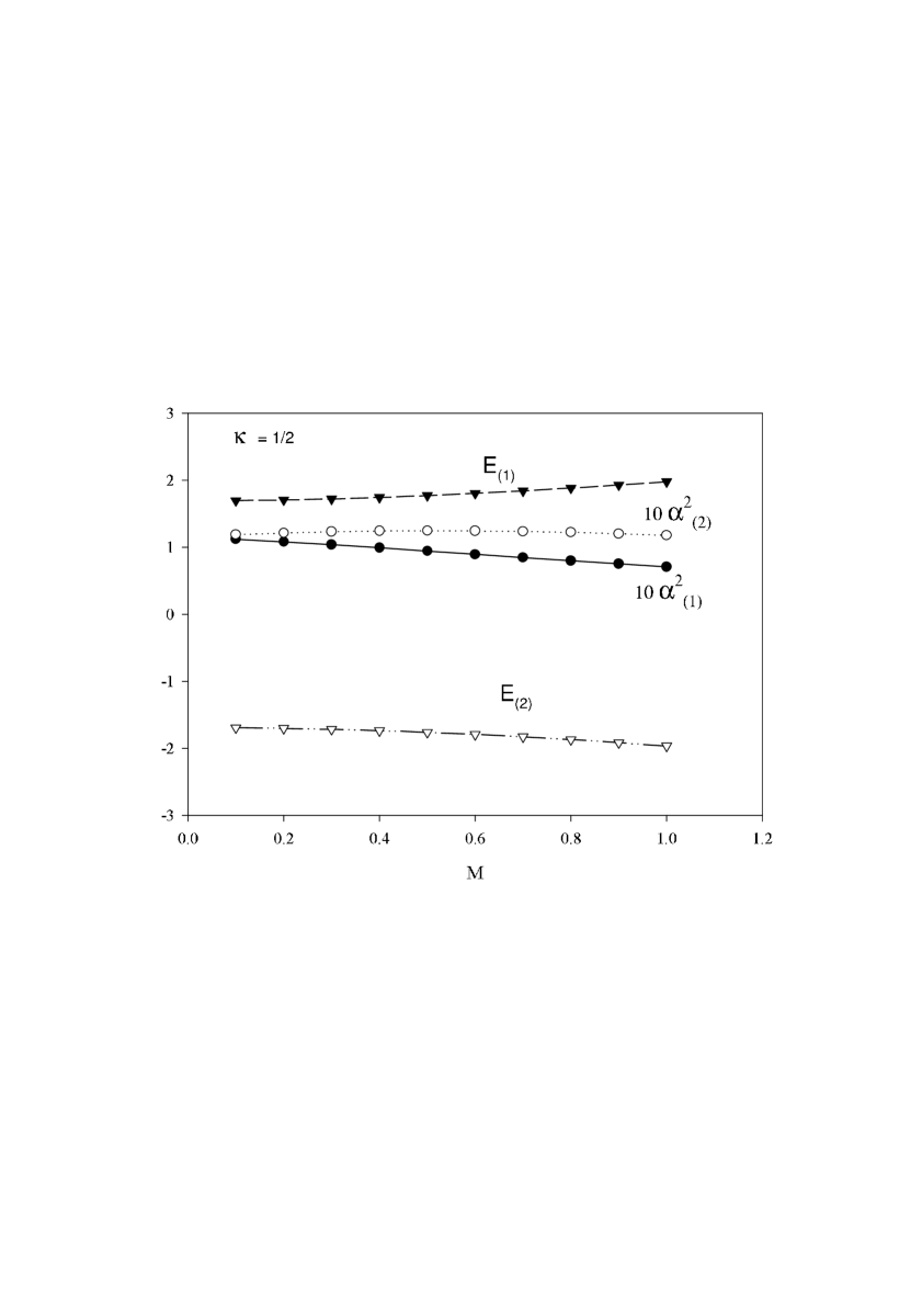
Figure 1: The values of $\alpha$ and of the energy are plotted as functions of M in the case $\kappa=1/2$.

Already for $n=1$ the final equation relating $\alpha,M,\kappa$ is very involved. The allowed values of $\alpha$ with $M,\kappa$ fixed can be determined numerically. For the case $\kappa=1/2$, there are four possible values of $\alpha$ and two corresponding values of the energy $\varepsilon$. They are presented on Fig.1 for $M\in[0,1]$. For $\kappa=3/2$ the picture is qualitatively similar to Fig.1.

4.2 Extended Dirac oscillators

The case treated in the previous section is physically important, but we have seen that no algebraic solution can be constructed for generic values of the Coulomb and oscillator coupling constants, respectively $\alpha,\tilde{B}$. We would like to construct a model where algebraic solutions exist for generic values of the Coulomb and oscillator constants. In this purpose, we consider Eq.(2) with an extended choice for oscillator’s parameters. Namely, we set

$$V(r)={\alpha\over r}\qquad,\qquad W(r)=\beta_{1}r\qquad E(r)=\gamma_{0}+\gamma_{1}r\ \ .$$ (23)

This choice constitutes one possible relativistic generalisation of the non-relativistic problem considered in [3] Here the Coulomb interaction is supplemented by two types of confining (i.e. linear in $r$) interactions. Note that, adding a constant to the potential $W(r)$ is equivalent to redefine the mass $M$. To the contrary, the constant $\gamma_{0}$ cannot be eliminated by a redefinition of the physical quantities.

We look for solutions of the form

$$\left(\begin{array}[]{c}f\\ g\end{array}\right)=r^{\theta}\exp(-{\lambda_{2}\over 2}r^{2}-\lambda_{1}r)\left(\begin{array}[]{c}\tilde{p}\\ \tilde{q}\end{array}\right)$$ (24)

where $\theta,\lambda_{1},\lambda_{2}$ are constants and $\tilde{p}(r),\tilde{q}(r)$ are chosen as polynomials in $r$. Inserting (24) into (2), we obtain the counterpart of (17) with

$$\tilde{H}=\left(\begin{array}[]{cc}D-\lambda_{2}r^{2}-\lambda_{1}r+\theta-\kappa+\gamma_{0}r+\gamma_{1}r^{2}&\beta_{1}r^{2}-\alpha+r(M-\varepsilon)\\ \beta_{1}r^{2}+\alpha+r(M+\varepsilon)&D-\lambda_{2}r^{2}-\lambda_{1}r+\theta+\kappa-\gamma_{0}r-\gamma_{1}r^{2}\end{array}\right)$$ (25)

where $D$ is the dilatation operator $D=r\frac{d}{dr}$. Transforming the system according to

$$U^{-1}\tilde{H}U\left(\begin{array}[]{c}\tilde{p}\\ \tilde{q}\end{array}\right)=0\ \ ,\ \ U=\left(\begin{array}[]{cc}\cos\omega&-\sin\omega\\ \sin\omega&\cos\omega\end{array}\right)$$ (26)

with $R=\sqrt{\gamma_{1}^{2}+\beta_{1}^{2}}$, $\omega=(1/2)\arctan(\beta_{1}/\gamma_{1})$. we obtain the following conditions for polynomial solutions to exist:

$$\lambda_{2}=R\quad,\quad\lambda_{1}=\frac{\beta_{1}M+\gamma_{0}\gamma_{1}}{R}$$ (27)

with

$${\rm deg}\ \tilde{p}=n\quad,\quad{\rm deg}\ \tilde{q}=n-1\ .$$ (28)

The final equations for $\tilde{p},\tilde{q}$ then read

$$(D+A_{2})\tilde{p}+(A_{1}r+A_{0})\tilde{q} =0$$ (29)

$$(D+C_{2}r^{2}+C_{1}r+C_{0})\tilde{q}+(D_{1}r+D_{0})\tilde{p} =0$$

where

$$A_{2} =\theta-\frac{\gamma_{1}\kappa}{R}$$ (30)

$$A_{1} =\gamma_{1}^{2}\frac{(\varepsilon-M)}{\beta_{1}R}+\gamma_{1}\frac{(\beta_{1}\gamma_{0}+\varepsilon R-MR)}{\beta_{1}R}+\frac{\beta_{1}\varepsilon+\gamma_{0}R}{R}$$

$$A_{0} =\gamma_{1}^{2}\frac{\alpha}{\beta_{1}R}+\gamma_{1}\frac{(\alpha R-\beta_{1}\kappa)}{\beta_{1}R}+\frac{\alpha\beta_{1}-\kappa R}{R}$$

$$C_{2} =-2R$$

$$C_{1} =-2\frac{\beta_{1}M+\gamma_{0}\gamma_{1}}{R}$$

$$C_{0} =\frac{\gamma_{1}\kappa+\theta R}{R}$$

$$D_{1} =-(\gamma_{1}^{2}\frac{M-\varepsilon}{\beta_{1}R}+\gamma_{1}\frac{\varepsilon R-MR-\beta_{1}\gamma_{0}}{\beta_{1}R}+\frac{\gamma_{0}R-\beta_{1}\varepsilon}{R})$$

$$D_{0} =-\gamma_{1}^{2}\frac{\alpha}{\beta_{1}R}+\gamma_{1}\frac{\alpha R+\beta_{1}\kappa}{\beta_{1}R}+\frac{\kappa R-\alpha\beta_{1}}{R}$$

Eq. (29) with (28) leads to a set of $2n+3$ algebraic equations in $2n+2$ parameters ($\theta,E$ and $2n$ coefficients for $\tilde{p}$ and $\tilde{q}$); so it cannot be solved for generic values of the physical coupling constants $\alpha,\beta_{1},\gamma_{0},\gamma_{1},M$. However, considering one of these physical parameters as free (e.g. the parameter $\gamma_{0}$) we are lead to consistent equations which, in principle, possess solutions and fix one energy level $\varepsilon$ and the constant $\gamma_{0}$ as functions of the parameters $\alpha,\beta_{1},\gamma_{1},M$ and of $\kappa$.

The analysis of terms of highest and lowest degrees in $r$ in these linear equations lead respectively to the following condition for the eigenvectors

$$\tilde{p}=x^{n}+o(x^{n-1})\ \ \ ,\ \ \ \tilde{q}=-\frac{n+A_{2}}{A_{1}}x^{n-1}+o(x^{n-2}).$$ (31)

$$\varepsilon^{2}=2(R(n+\theta)-\gamma_{1}\kappa)+\frac{M^{2}\gamma_{1}^{2}+\beta_{1}^{2}\gamma_{0}^{2}-2M\beta_{1}\gamma_{0}\gamma_{1}}{R^{2}}\ \ \ ,\ \ \ \theta=\sqrt{\kappa^{2}-\alpha^{2}}\quad,\quad\kappa=\pm 1,\pm 2,\dots$$ (32)

The first of these equations can be used to determine $\varepsilon$ while the second allows one to determine the parameter $\theta$.

We have analysed the equations numerically for the case $n=1,\kappa=1$ corresponding to the ground state of the equation. Fixing symbolically $\gamma_{1}=3$,$\beta_{1}=4$ and $M=1$ we found that two possible values occur for the parameter $\gamma_{0}$. These values are real for $\alpha\in[0.097,0.92]$ and become complex outside that interval. The two branches of values are presented on Fig. 2.

The results obtained above suggest that the reduced spherically symmetric Hamiltonian is equivalent to an operator preserving the vector space $P(n-1)\oplus P(n)$. However, in spite of our efforts, we could not find a change of basis making this job and we believe that it is not. Nevertheless, if we combine the two equations in order to obtain decoupled second order equations for the two components of the spinor, we got linear operators of the form [11]

$$T\equiv(x^{2}+x_{0}x)\frac{d^{2}}{dx^{2}}+(-x^{2}(x+x_{0})+2\beta(x+x_{0}))\frac{d}{dx}+\varepsilon x(x+x_{0})+(b-c)x+bx_{0}$$ (33)

where

$$\tilde{\varepsilon}=\varepsilon^{2}-M^{2}-\kappa-\gamma-1\ \ ,\ \ b=2\varepsilon\alpha+(\kappa-\gamma)\frac{\varepsilon+M}{\alpha}\ \ ,\ \ c=\frac{\alpha}{\varepsilon+M}+(\kappa-\gamma)\frac{\varepsilon+M}{\alpha}$$ (34)

A necessary condition for the equation $TQ_{n}(x)=0$ to possess polynomial solution of degree $n$ in $x$ requires $\tilde{\varepsilon}=n$, quantizing the possible values of the energy. Once this is fixed, the operator can be set in the form

$$T=-x^{2}(x\frac{d}{dx}-n)-x_{0}x(x\frac{d}{dx}-n)+(b-c)x+S_{QES}=xT_{QES}+S_{QES}\ \$$ (35)

where $T_{QES},S_{QES}$ can be expressed in terms of the three basic generators $J^{+}_{n}=x(x\frac{d}{dx}-n)$, $J^{0}_{n}=(x\frac{d}{dx}-\frac{n}{2})$ , $J^{-}_{n}=\frac{d}{dx}$. This provides an alternative demonstation that $T$ can be expressed as an element of the envelopping algebra of osp(2,2), as pointed out recently in [7]. Once set in this form, the equation $TQ_{n}(x)=0$ leads to a system of $n+2$ linear equations in $n$ parameters ($n$ parameters in $Q_{n}$ , remember that the parameter $\gamma$ is fixed by $\gamma=\sqrt{\kappa^{2}-\alpha^{2}}$).

So naively, one would expect the equations to fix two conditions among the coupling constants of the model, contrasting with the counting of equations and parameters done with the systems of first order equations.

However, due to the fact that the second order equation is obtained from the first order ones, it turns out that the two extra conditions are indeed consistent with each other and there is effectively one extra relation. To our knowledge, this property is not at all apparent by just looking at the second order equation. This construction can nevertheless be used to extend the class of one dimensional quasi exactly solvable operators away from the class of operators which are directly expressible in the envelopping algebra of sl(2,R).

5 Outlook

We have shown that algebraic solutions of the Dirac + Coulomb + confining potential equations (with both Dirac oscillator and normal harmonic potentials) can admit some explicit bound states. A generalisation of the Dirac oscillator has been obtained which can be completely solved algebraically (i.e. it is exactly solvable) and posseses a hidden algebra related to osp(2,2).

The mixed case, with both oscillators and Coulomb-terms, leads generally to an overdetermined systems of equations but, allowing one of the coupling constants to be “free”, leads to a sufficient number parameters and the system of equations can be solved consistently by means of algebraic techniques. We believe that our results could be generalized by including screened potentials and using the ideas of [5].

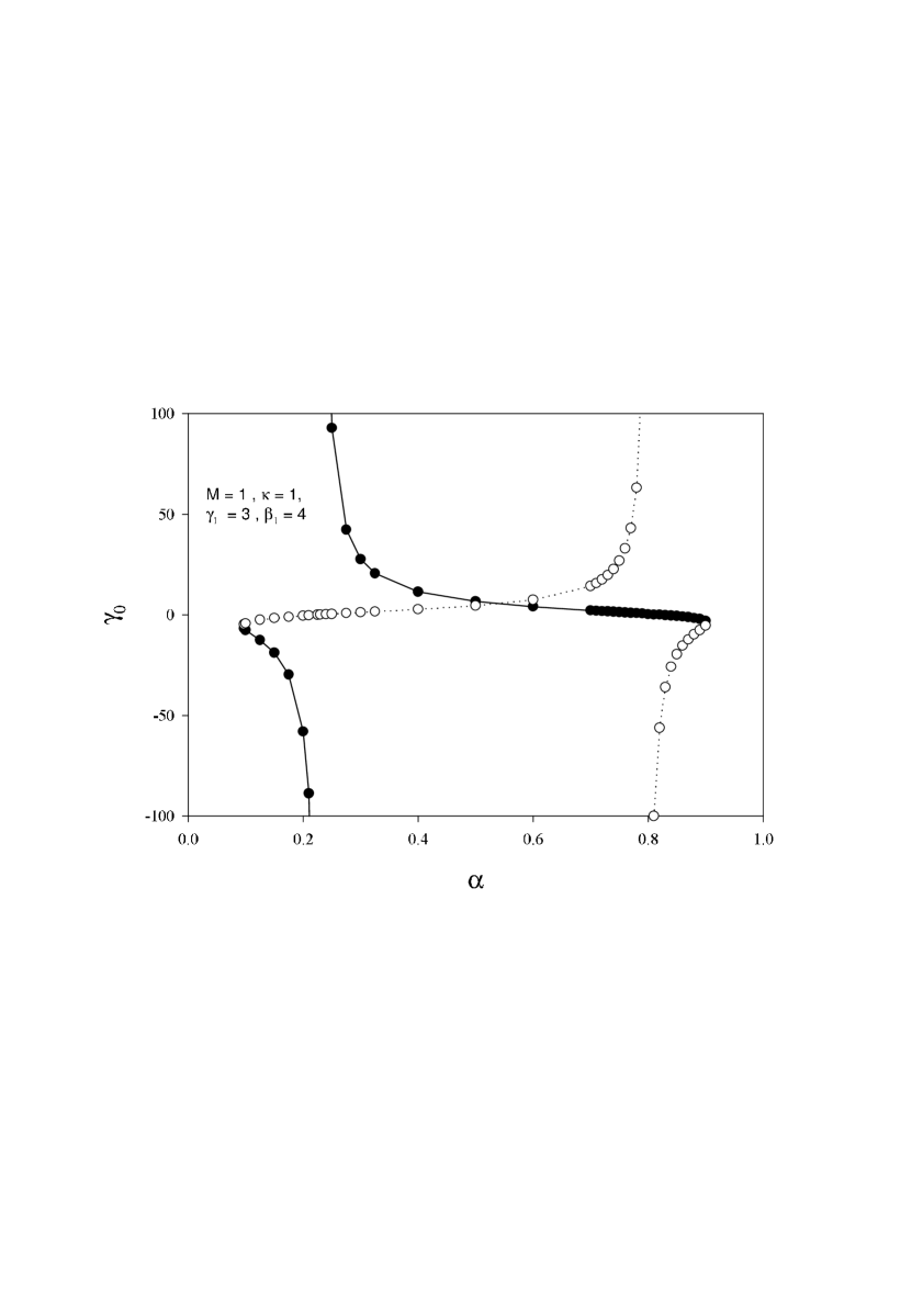
Figure 2: The two possibles values of the parameter $\gamma_{0}$ are plotted as functions of the Coulomb coupling constant $\alpha$ for the ”ground state“ solution corresponding to mixed oscillators.

References

- [1] A.V. Turbiner, Comm. Math. Phys.118, 467 (1988).
- [2] A.G.Ushveridze, ”Quasi exact solvability in quantum mechanics”, Institute of Physics Publishing, Bristol and Philadelphia (1993).
- [3] A.V. Turbiner, Phys. Rev. A50, 5335 (1994).
- [4] Y. Brihaye, P. Kosinski, Mod. Phys. Lett. A 14, 2579 (1999).
- [5] M.Znojil, Mod. Phys. Lett. A 14, 863 (1999).
- [6] C.-L. Ho and P. Roy, Annals of Physics 312, 161 (2004)
- [7] C.-M. Chiang and C.-L Ho, Quasi-Exact Solvability of Planar Dirac Electron in Coulomb and Magnetic Fields, quant-ph/0501035.
- [8] M. V. Shifman and A. V. Turbiner, Commun. Math. Phys. 126 (1989) 347.
- [9] V. Villalba, J. Math. Phys. 36, 3332 (1995).
- [10] G. Torres del Castillo, L. Cortes-Curantli, J. Math. Phys. 38 (1997) 2996.
- [11] C.-M. Chiang and C.-L Ho, J. Math. Phys. 43 (2002) 43.
- [12] Q.-G. Lin, J. Phys. G 25, 1795 (1999).