Revealing virtual processes of a quantum Brownian particle in the phase space

Abstract

The short time dynamics of a quantum Brownian particle in a harmonic potential is studied in the phase space. An exact non-Markovian analytic approach to calculate the time evolution of the Wigner function is presented. The dynamics of the Wigner function of an initially squeezed state is analyzed. It is shown that virtual exchanges of energy between the particle and the reservoir, characterizing the non-Lindblad short time dynamics where system-reservoir correlations are not negligible, show up in the phase space.

1 Introduction

During the last decades applications based on the most radical predictions and features of quantum mechanics, namely the existence of quantum superpositions and the entanglement, have been conceived [1]. Both of these features lie at the root of a new class of quantum technologies exploiting the coherent manipulation of quantum systems. Such process involves very delicate procedures since the inevitable interaction of the quantum systems with their surrounding leads to loss of information and causes two types of phenomena countering the coherent control of quantum systems: decoherence and dissipation. Decoherence, which is the loss of phase coherence between superpositions of quantum states, and dissipation, which is the leakage of population from the system to the environment, are the major enemies of quantum technologies. In order for quantum technologies to emerge, decoherence and dissipation need to be defeated or controlled, and for that they must be completely understood.

The theory of open quantum systems deals with the microscopic description of quantum systems interacting with their surroundings [2]. It is of crucial importance to incorporate methods and tools of the theory of open quantum systems to the investigation of quantum technologies. Understanding and being able to describe the effects of the environment on quantized systems is the pre-requisite for the implementation of realistic applications.

The exact analytic description of the dynamics of an open system is not an easy task. Commonly a series of approximations are necessary in order to obtain treatable equations of motions for the density matrix of the open system. Typical approximations are the weak coupling and the Markovian approximations. The first one assumes that the coupling between the system and the environment is weak while the second one assumes that the correlations between system and environment are negligible.

The miniaturization process which has lead to the possibility of manipulating coherently quantum systems, exploiting the crucial features of quantum theory, has been accompanied by the need of speeding up the quantum engineering methods. This is because the quantum properties of the systems, such as entanglement, gets eventually destroyed by the interaction with the environment. The description of the short time dynamics of an open quantum system requires exact approaches which do not rely on the Markovian approximation. Recently, a non-Markovian description of quantum computing showing the limits of the Markovian approach has been presented [3]. Moreover, for many solid state systems, the properties of the reservoirs are such that the Markovian assumption does not hold at any time. This is e.g. the case of atom lasers and photonic band gap materials [4]. Therefore the study of the dynamics of paradigmatic open quantum systems using non-Markovian analytical approaches is crucial for the development of prototypes of quantum devices which are the building blocks of tomorrow’s technologies.

In this paper I focus on an ubiquitous open quantum system, namely the damped harmonic oscillator or quantum Brownian particle in a harmonic potential [5]. Recently an analytic approach for solving the non-Markovian master equation for this system via the simmetrically ordered characteristic function has been presented [6], and its dynamics has been studied [7]. One of the new dynamical features discovered in Ref. [7] is the existence of a regime characterized by virtual exchanges of energy between the system oscillator and its surrounding. Here we focus on this regime and we present a method to calculate exactly the non-Markovian time evolution of the Wigner function of an initially squeezed state of the oscillator. It has been demonstrated in Ref. [8] that the regime considered in this paper may be experimentally simulated with single trapped ions. It is worth recalling that, for these systems, measurements of the Wigner function have been performed in the experiments [9].

The paper is structured as follows. In Sec.2 we review the properties of the system, introducing the master equation and its solution. Section 3 contains the main result of the paper, namely the derivation of the exact dynamics of the Wigner function for an initially squeezed state. Finally Sec. 4 presents conclusions.

2 The system and the master equation

The reduced density matrix $\rho_{S}$ describing the dynamics of the quantum Brownian particle obeys, in the secular approximation, to the following non-Markovian master equation [10]

$$\frac{d\rho_{S}}{dt}= - \frac{\Delta(t)+\gamma(t)}{2}\left[a^{{\dagger}}a\rho_{S}-2a\rho_{S}a^{{\dagger}}+\rho_{S}a^{{\dagger}}a\right]$$ (1)

$$- \frac{\Delta(t)-\gamma(t)}{2}\left[aa^{{\dagger}}\rho_{S}-2a^{{\dagger}}\rho_{S}a+\rho_{S}aa^{{\dagger}}\right],$$

where we have introduced the bosonic annihilation and creation operators $a$ and $a^{{\dagger}}$, respectively. The coefficients $\Delta(t)$ and $\gamma(t)$ are the diffusion and dissipation coefficients, and they are defined in terms of the noise and dissipation kernels, respectively [7]. The form of Eq. (1) is similar to the Lindblad form [11], with the only difference that the coefficients appearing in the master equation are here time dependent. We say that this master equation is of Lindblad-type when the coefficients $\Delta(t)\pm\gamma(t)$ are positive at all times [12]. Note, however, that Lindblad type master equations, contrarily to master equations of Lindblad form, in general do not satisfy the semigroup property.

For a high temperature reservoir with Ohmic spectral density the analytic expression of the diffusion and dissipation coefficients is the following

$$\Delta(t) = 2g^{2}kT\frac{r^{2}}{1+r^{2}}\left\{1-e^{-\omega_{c}t}\left[\cos(\omega_{0}t)-(1/r)\sin(\omega_{0}t)\right]\right\},$$ (2)

and

$$\gamma(t)=\frac{g^{2}\omega_{0}r^{2}}{1+r^{2}}\Big{[}1\!-\!e^{-\omega_{c}t}\cos(\omega_{0}t)\!-re^{-\omega_{c}t}\sin(\omega_{0}t)\Big{]},$$ (3)

with $g$ system-reservoir coupling constant, $r=\omega_{c}/\omega_{0}$, $\omega_{c}$ cutoff frequency of the spectrum of the reservoir, $\omega_{0}$ frequency of the system oscillator, and $k$ Boltzmann constant.

The solution for the density matrix of the system may be written in terms of the simmetrically ordered characteristic function $\chi_{t}(\xi)$ at time $t$, also known as quantum characteristic function (QCF), defined through the equation [13]

$$\rho_{S}(t)=\frac{1}{2\pi}\int\chi_{t}(\xi)\>e^{\left(\xi a^{{\dagger}}-\xi^{*}a\right)}d^{2}\xi.$$ (4)

Using Eq. (4) one may solve the master equation given by Eq. (1) by means of a method based on the algebraic properties of the time evolution superoperator. Indeed we have proved that the form of the time evolution superoperator may be factorized into three parts allowing the derivation of an exact analytic solution [6]. The QCF of the system considered here is given by

$$\chi_{t}(\xi)=e^{-\Delta_{\Gamma}(t)|\xi|^{2}}\chi_{0}\left[e^{-\Gamma(t)/2}e^{-i\omega_{0}t}\xi\right],$$ (5)

with $\chi_{0}$ QCF of the initial state of the system. The quantities $\Delta_{\Gamma}(t)$ and $\Gamma(t)$ appearing in Eq. (5) are defined in terms of the diffusion and dissipation coefficients $\Delta(t)$ and $\gamma(t)$ respectively as follows

$$\Gamma(t) = 2\int_{0}^{t}\gamma(t_{1})\>dt_{1},$$ (6)

$$\Delta_{\Gamma}(t) = e^{-\Gamma(t)}\int_{0}^{t}e^{\Gamma(t_{1})}\Delta(t_{1})dt_{1}.$$ (7)

It is well known that non-Markovian features usually occur in the dynamics for times $t\ll\tau_{R}=2\pi/\omega_{c}$, with $\tau_{R}$ reservoir correlation time. For quantum optical systems, since $\omega_{c}\gg\omega_{0}$, and $\omega_{0}$ is an optical frequency, deviations from the Markovian dynamics appear for very short times, usually too short to be measured in the experiments. With trapped ion systems $\omega_{0}\simeq 10^{7}$Hz, and therefore non-Markovian features would appear for times $t\ll 0.1\mu$s. This is the reason why typical trapped ion experiments, wherein the time scales go from $1$ to $100\mu$s, show a Markovian behaviour. In the trapped ion context, however, it is possible to engineer an artificial reservoir wherein parameters as the system-reservoir coupling and the cutoff frequency can be controlled [14]. With an appropriate engineered reservoir one may force non-Markovian features to appear by ‘detuning’ the trap frequency from the reservoir spectral density [8]. This corresponds, for example, to the case in which $r=\omega_{c}/\omega_{0}\ll 1$, e.g. $r=0.1$. In this case the reservoir correlation time is bigger than the period of oscillation of the ion, $\tau_{R}=2\pi\mu$s, and therefore the non-Markovian features show up in the time evolution and can be measured. At the moment, in fact, this would require a slight modification of the current experimental apparatus used in the group of David Wineland at NIST since a switch should be positioned between the filters, which are inside the vacuum chamber, and the trap electrode [15].

In the following we will pay special attention to the experimentally realizable regime $r\ll 1$. It is easy to verify that for $r\ll 1$ the coefficients $\Delta(t)\pm\gamma(t)$ appearing in the master equation, with $\Delta(t)$ and $\gamma(t)$ given by Eqs. (2)-(3), take negative values [see, e.g. Ref. [12]]. In this case, therefore, the master equation is of non-Lindblad-type. It is worth underlining that, in this regime and for the system here considered, the density matrix is completely positive at all times $t$ while the semigroup property of the generator of the dynamics is clearly violated [2]. Under these conditions virtual exchanges of energy between system and reservoir appear due to the system-reservoir correlations. These virtual processes show up in the dynamics of the mean energy of the system in the form of oscillations (see Fig. 1), and they are a clear signature of the break down of the semigroup property. The virtual exchanges of excitations characterize the regime $r<1$ since in this regime the period $T=2\pi/\omega_{0}$ of the system oscillator is smaller than the reservoir correlation time $\tau_{R}=2\pi/\omega_{c}$. Due to the time-energy uncertainty principle, for times $t<T$, a virtual process consisting in the absorption of a quantum of energy $\hbar\omega_{0}$ from a high temperature reservoir and consequent re-emission of the same quantum of energy may occur. In Fig. 1 we see the oscillation in the mean number of quanta $\langle n\rangle$ of the system oscillator for an initial state having $\langle n\rangle(t=0)=3$, during the time interval $0<\tau<1$, with $\tau=\omega_{c}t$, for $r=0.05$. Note that the period of the system oscillator, in the same time units, is $\omega_{c}T=2\pi r\simeq 0.3141$, which coincides exactly with the period of the oscillations displayed in Fig.1.

In the following section we will see how virtual processes influence the dynamics of the Wigner function.

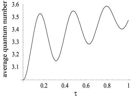
Figure 1: Time evolution of the average quantum number $\langle n\rangle$ vs the dimensionless time $\tau=\omega_{c}t$ for an initial state having excitation number $\langle n\rangle(t=0)=3$. The parameters used are the following $r=0.05$, $g=0.1$, $\omega_{c}/2\pi KT=3\cdot 10^{-5}$

.

3 The time evolution of the Wigner function

The Wigner function is the Fourier transform of the simmetrically ordered characteristic function

$$W(\alpha)=\frac{1}{\pi^{2}}\int_{-\infty}^{\infty}d^{2}\xi\chi(\xi)e^{\alpha\xi^{*}-\alpha^{*}\xi}.$$ (8)

Inserting Eq.(5) into the previous equation one obtains

$$W_{t}(\alpha)=\frac{1}{\pi^{2}}\int_{-\infty}^{\infty}\!\!\!\!d^{2}\xi\,e^{-\Delta_{\Gamma}(t)|\xi|^{2}}\,e^{\alpha\xi^{*}-\alpha^{*}\xi}\chi_{0}(e^{-\Gamma(t)/2}e^{-i\omega_{0}t}\xi).$$ (9)

Inserting the inverse Fourier transform of Eq. (8) into Eq.(9) gives

$$W_{t}(\alpha)=\frac{1}{\pi^{2}}\int_{-\infty}^{\infty}\,d^{2}\alpha_{0}W_{0}(\alpha_{0})$$

$$\int_{-\infty}^{\infty}\,d^{2}\xi\,e^{-\Delta_{\Gamma}(t)|\xi|^{2}}\,e^{b(t,\alpha,\alpha_{0})\xi^{*}-b^{*}(t,\alpha,\alpha_{0})\xi}$$

$$=\frac{1}{\pi}\int_{-\infty}^{\infty}d^{2}\alpha_{0}W_{0}(\alpha_{0})\frac{\exp\left[-\frac{|b(t,\alpha,\alpha_{0})|^{2}}{\Delta_{\Gamma}(t)}\right]}{\Delta_{\Gamma}(t)}$$

$$\equiv\frac{1}{\pi}\int_{-\infty}^{\infty}d^{2}\alpha_{0}W_{t}(\alpha|\alpha_{0})W_{0}(\alpha_{0}),$$ (10)

with

$$b(t,\alpha,\alpha_{0})=\alpha-\alpha_{0}e^{-\Gamma(t)/2}e^{i\omega_{0}t}.$$ (11)

In the derivation of Eq. (10) we have used the property that the Fourier transform of a Gaussian is a Gaussian. The quantity $W_{t}(\alpha|\alpha_{0})$ is the propagator which, for $t\rightarrow 0$, tends to the delta function $\delta(\alpha-\alpha_{0})$.

If the state of the input field is a coherent state $|\alpha_{0}\rangle$, then the integral appearing in Eq. (10) may be easily calculated since the Wigner function of the initial coherent state is a Gaussian. In this case the Wigner function at time $t$ reads as follows

$$W_{t}(\alpha)=\frac{1}{\pi\left[\Delta_{\Gamma}(t)+1/2\right]}\exp\left[\frac{\left|\alpha_{0}e^{-\Gamma(t)/2}e^{-i\omega_{0}t}-\alpha\right|^{2}}{\Delta_{\Gamma}(t)+1/2}\right].$$ (12)

Having in mind this equation, and with the help of Eqs. (6)-(7) and (2)-(3), it is possible to show that the system-reservoir interaction spreads the initial Wigner function. Breathing of the Wigner function, that is the oscillation in its spread, appears in correspondence of the virtual processes. This is a dynamical feature which is absent both in the Markovian dynamics of the damped harmonic oscillator and in the Lindblad-type non-Markovian dynamics. Indeed, in both the previous regimes, the spread in the Wigner function simply increases, linearly in time in the Markovian case, and quadratically in time in the non-Markovian Lindblad-type case.

We now consider the case of an initially squeezed state. The initial QCF for squeezed coherent state is

$$\chi_{0}(\xi)=\exp\left[-\frac{1}{2}|\xi C_{s}-\xi^{*}e^{-i\phi}S_{s}|^{2}+i(\xi^{*}\alpha_{0}^{*}+\xi\alpha_{0})\right].$$ (13)

Here $C_{s}=\cosh(s)$ and $S_{s}=\sinh(s)$, $\alpha_{0}$ is the displacement of the initial state of the oscillator and $z=se^{-i\phi}$ is the squeezing argument. For this initial condition the explicit integration appearing in Eq.(10) is more difficult to carry out. In the case of an initial squeezed vacuum state ($\alpha_{0}=0$) with squeezing angle $\phi=0$, the Wigner function at time $t$ has the form

$$W_{t}(\alpha) = \frac{1}{\pi^{2}}\int_{-\infty}^{\infty}\,d^{2}\xi\,e^{-\Delta_{\Gamma}(t)|\xi|^{2}}e^{\left(\alpha\xi^{*}-\alpha^{*}\xi\right)}$$ (14)

$$\exp\left[-\frac{1}{2}e^{-\Gamma(t)}|e^{-i\omega_{0}t}\xi C_{s}-e^{i\omega_{0}t}\xi^{*}S_{s}|^{2}\right].$$

Looking at the previous equation one realizes that what we need to calculate is the Fourier transform of the product of two functions

$$W_{t}(\alpha)=\frac{1}{\pi^{2}}\int_{-\infty}^{\infty}\,d^{2}\xi\,f_{1}(\xi)\,f_{2}(\xi)e^{\left(\alpha\xi^{*}-\alpha^{*}\xi\right)},$$ (15)

where

$$f_{1}(\xi) = e^{-\Delta_{\Gamma}(t)|\xi|^{2}},$$ (16)

$$f_{2}(\xi) = \exp\left[-\frac{1}{2}e^{-\Gamma(t)}|e^{-i\omega_{0}t}\xi C_{s}-e^{i\omega_{0}t}\xi^{*}S_{s}|^{2}\right].$$ (17)

If we denote the Fourier transform $\mathcal{F}$ of the functions $f_{1}(\xi)$ and $f_{2}(\xi)$ as follows, $F_{1}=\mathcal{F}(f_{1})$ and $F_{2}=\mathcal{F}(f_{2})$, we can recast $W_{t}$ in the form

$$W_{t}(\alpha)=F_{1}\ast F_{2}$$ (18)

where $\ast$ denotes the convolution. We now extend the method developed in Ref. [16] for the calculation of the Wigner function of an initial squeezed state to the non-Markovian case we are dealing with in this paper. Carrying out the calculations, in a frame rotating with $\omega_{0}$, one obtains

$$W_{t}(\alpha) = M\exp\left[\frac{-2\alpha_{x}^{2}}{2\Delta_{\Gamma}(t)+e^{-\Gamma(t)}(C_{2s}+S_{2s})^{-1}}\right]$$ (19)

$$\times \exp\left[\frac{-2\alpha_{y}^{2}}{2\Delta_{\Gamma}(t)+e^{-\Gamma(t)}(C_{2s}-S_{2s})^{-1}}\right]$$

$$= M\exp\left[\frac{-\alpha_{x}^{2}}{(\Delta x)^{2}(t)}+\frac{-\alpha_{y}^{2}}{(\Delta y)^{2}(t)}\right]$$

Here, $\alpha_{x}$ and $\alpha_{y}$ are the real and imaginary parts of $\alpha$, $M$ is a time dependent normalization constant, and

$$(\Delta x)^{2}(t)=\Delta_{\Gamma}(t)+\frac{e^{-\Gamma(t)}e^{-2s}}{2},$$ (20)

$$(\Delta y)^{2}(t)=\Delta_{\Gamma}(t)+\frac{e^{-\Gamma(t)}e^{2s}}{2},$$ (21)

are the variances of the dimensionless quadratures

$$x = \frac{1}{\sqrt{2}}\left(a+a^{{\dagger}}\right),$$ (22)

$$y = \frac{-i}{\sqrt{2}}\left(a-a^{{\dagger}}\right).$$ (23)

At $t=0$, $(\Delta x)^{2}(0)=e^{-2s}/2\equiv\sigma^{2}/2$ and $(\Delta y)^{2}(0)=e^{2s}/2\equiv 1/2\sigma^{2}$. We consider an initial state displaying squeezing in the $x$ quadrature, i.e., in the trapped ion case, a state squeezed along the $x$ direction of the trap. This corresponds to $\sigma<1$ since the $x$-squeezing is characterized by $(\Delta x)^{2}<0.5$. In Fig. 2 we plot the time evolution of $(\Delta x)^{2}$ as a function of the dimensionless time $\tau=\omega_{c}t$, for an initial squeezed state with $\sigma^{2}=0.1$, together with the contour plot of the Wigner function at four different time instants, $\tau=0$, $\tau=0.15$, $\tau=0.3$ and $\tau=0.45$.

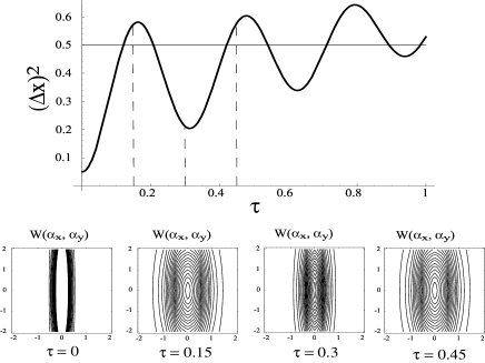
Figure 2: Time evolution of $(\Delta x)^{2}$ vs the dimensionless time $\tau=\omega_{c}t$. The parameters used are the following $\sigma^{2}=0.1$, $r=0.05$, $g=0.1$, $\omega_{c}/2\pi KT=3\cdot 10^{-5}$. The insets at the bottom of the figure show the contour plot of the Wigner function at times $\tau=0$, $\tau=0.15$, $\tau=0.3$, $\tau=0.45$.

The graphic shows that, due to the interaction with a high temperature reservoir, the variance of the $x$ dimensionless operator, defined by Eq.(22), increases from its initial value $(\Delta x)^{2}(0)=0.05$. For short times, however, the dynamics is governed by oscillations between a squeezed state and a non-squeezed state due to the occurrence of virtual exchanges of excitations between the system oscillator and the reservoir. As clearly shown in the figure, at $\tau\simeq 0$ and $\tau\simeq 0.15$ the system is in a squeezed state [$(\Delta x)^{2}(0)<0.5$] while at $\tau\simeq 0.3$ and $\tau\simeq 0.45$ the system is in a non-squeezed state. By using the calculation we have carried out in this paper for the time evolution of an initially squeezed state, see Eq. (19), we can also plot the contours of the Wigner function at these time instants [see insets at the bottom of of Fig. (2)]. More in general Eq. (19), together with Eqs. (6)-(7) and (2)-(3), tell us that the Wigner function of an initially squeezed state, in the phase space, spread along both the $\alpha_{x}$ and the $\alpha_{y}$ axes and eventually approaches the Wigner function of a thermal state. For times shorter than the reservoir correlation time, however, in the non-Lindblad regime both $(\Delta x)^{2}$ and $(\Delta y)^{2}$ oscillate, so that if the system is initially in a squeezed state along the $x$ ($y$) direction then this may result in $x$ ($y$) squeezing oscillations.

4 Conclusions

In this paper I have studied the non-Markovian dynamics of a quantum harmonic oscillator in phase space. I have presented a method to calculate the Wigner function of an initially squeezed state of motion for short times, when the system-reservoir correlations dominate the dynamics. The solution obtained is used to investigate the non-Lindblad regime, characterized by virtual exchanges of energy between the system and the reservoir. It is shown that the virtual processes are responsible for the oscillations between a squeezed and a non-squeezed state of the system. It is worth recalling that the non-Lindblad regime is experimentally realizable with artificial reservoirs in the trapped ion context. In this context, moreover, the Wigner function is experimentally measurable. Therefore, by measuring the Wigner function, it is possible to reveal the virtual processes characterizing the non-Markovian non-Lindblad dynamics, and in particular the squeezing-nonsqueezing oscillations. The result here presented contributes to the understanding of the short time dynamics of an ubiquitous model of an open quantum system, namely the damped harmonic oscillator, and hence it is also of potential interest for quantum technologies. In fact in many solid-state physical systems promising for building prototypes of quantum devises the Markovian approximation does not hold. Moreover, if one is interested to very short system dynamics one needs to abandon the Markovian assumption. The result has also implications in the study of fundamental issues of quantum measurement theory since there are indications that the non-Lindblad regime may correspond to a situation in which no measurement scheme interpretation of the non-Markovian stochastic process exists.

References

References

- [1] Nielsen M A and Chuang I L 2000 Quantum Computation and Quantum Information (Cambridge: Cambridge University Press).
- [2] Breuer H-P and Petruccione F 2002 The Theory of Open Quantum systems (Oxford: Oxford University Press) .
- [3] Alicki R, Horodecki M, Horodecki P and Horodecki R 2002 Phys. Rev. A 65 062101; Alicki R et al 2004 Phys. Rev. A 70 010501.
- [4] Hope J J 1997 Phys. Rev. A 55 R2531; Moy G M, Hope J J, and Savage C M 1999 Phys. Rev. A 59 66; John S and Quang T 1994 Phys. Rev. Lett. 74 3419.
- [5] Haake F and Reibold R 1985 Phys. Rev. A 32 2462; Feynman R P and Vernon F L 1963 Ann. Phys. 24 118; Hu B L, Paz P, and Zhang Y 1992 Phys. Rev. D 45 2843; Ford G W and O’Connell R F 2001 Phys. Rev. D 64 105020; Grabert H, Schramm P, and Ingold G-L 1988 Phys. Rep. 168 115.
- [6] Intravaia F, Maniscalco S, and Messina A 2003 Phys. Rev. A 67 042108.
- [7] Maniscalco S, Piilo J, Intravaia F, Petruccione F, and Messina A 2004 Phys. Rev. A 70 032113.
- [8] Maniscalco S, Piilo J, Intravaia F, Petruccione F, and Messina A 2004 Phys. Rev. A 69 052101.
- [9] Leibfried D. et al. 1996 Phys. Rev. Lett. 77 4281.
- [10] For a detailed discussion on the approximations leading to this master equation see Intravaia F, Maniscalco S, and Messina A 2003 Eur. Phys. J. B 32 109.
- [11] Lindblad G 1976 Comm. Math. Phys. 48 119; Gorini V, Kossakowski A, and Sudarshan E C G 1976 J. Math. Phys. 17 821.
- [12] Maniscalco S, Intravaia F, Piilo J, and Messina A 2004 J. Opt. B: Quantum and Semiclass. Opt. 6 S98.
- [13] Barnett S M and Radmore P M 1997 Methods in Theoretical Quantum Optics (Oxford: Oxford University Press).
- [14] Myatt C J et al. 2000 Nature 403 269; Turchette Q A et al. 2000 Phys. Rev. A 62 053807.
- [15] David Wineland, private communication.
- [16] Matsuo K 1993 Phys. Rev. A 47 3337.