Entanglement Evolution in the Presence of Decoherence

Abstract

The entanglement of two qubits, each defined as an effective two-level, spin 1/2 system, is investigated for the case that the qubits interact via a Heisenberg XY interaction and are subject to decoherence due to population relaxation and thermal effects. For zero temperature, the time dependent concurrence is studied analytically and numerically for some typical initial states, including a separable (unentangled) initial state. An analytical formula for non-zero steady state concurrence is found for any initial state, and optimal parameter values for maximizing steady state concurrence are given. The steady state concurrence is found analytically to remain non-zero for low, finite temperatures. We also identify the contributions of global and local coherence to the steady state entanglement.

1 Introduction

Entanglement is a property of correlated quantum systems that cannot be accounted for classically. Entangled states of distinct (possibly interacting) quantum systems, which are those that cannot be factorized into product states of the subsystems, are of fundamental interest in quantum mechanics. The production of pairwise entangled states is an essential requirement for the operation of the quantum gates that make quantum information and quantum computation possible [1]. Considerable attention has been devoted to interacting Heisenberg spin systems [2, 3, 4, 5], which serve as a model for various solid state [6, 7, 8] or NMR [9, 10] quantum computation schemes and for simulating magnetic phenomena in condensed matter systems using atoms in optical lattices [11, 12]. Indeed, general Hamiltonians that include Heisenberg spin-spin interactions have been proposed as “generic” [13] or “ideal” [14] model Hamiltonians for quantum computation systems. A key question for entangled quantum states is the effect of decoherence due to the environment (see, e.g., [15, 16, 17, 18, 19] and references therein), which is not only a fundamental issue for quantum computation devices [20, 21] but also for the relation between quantum and classical physics [16, 22]. Although there have been many investigations of decoherence in recent years, careful investigation of well-understood model systems continue to produce surprises that add to fundamental understanding. For example, Yu and Eberly [23] have recently shown that the entanglement of a pair of non-interacting qubits in the presence of spontaneous decay of the upper states may decohere in a finite time instead of exponentially.

In this paper we examine decoherence due to both population relaxation and thermal effects for an entangled (and interacting) two qubit system. The Hamiltonian for our two-qubit system has the form of the well-known Heisenberg XY model for two interacting spins in the presence of an external magnetic field, where the effective magnetic field is defined by the energy separation of the two-level system that we associate with each (spin 1/2) qubit. As noted above, this form of Hamiltonian is very common in models for quantum computing [11, 12, 13, 14]. Our analysis of decoherence complements that of Ref. [23] by examining a system in which the qubits interact. For our two-qubit model system at zero temperature, we find that for any initial state, including the common one in which the two qubits are initially unentangled, the system reaches a steady state of pairwise entanglement in spite of population relaxation. The extent of steady-state entanglement is sensitive to both the spatial anisotropy of the interaction between qubits and to the energy level separation of the two levels associated with each qubit. To the extent that these two parameters can be varied in some particular physical realization of our model system, the magnitude of steady state entanglement may thus be controlled. We analyze both analytically and numerically the time-dependent evolution of the entanglement (as measured quantitatively by the concurrence [24, 25]) of our model two-qubit system for some typical initial states: a pure, separable initial state; a pure, entangled initial state; and a mixed initial state. We also obtain an analytic formula for the steady state concurrence that shows its dependence on both the system parameters and the decoherence rate and that enables us to specify optimal values for these parameters to achieve the maximum possible concurrence. In a separate section, we consider the case of finite temperature and present an analytic formula for the concurrence, which remains non-zero over a finite range of low temperatures. In our concluding section, we discuss some implications of these results.

2 Two-Qubit Hamiltonian

We note that the Hamiltonian of a Heisenberg chain of $N$ spin $\frac{1}{2}$ particles with nearest-neighbor interactions is [5]:

$$H=\sum_{n=1}^{N}(J_{x}S_{n}^{x}S_{n+1}^{x}+J_{y}S_{n}^{y}S_{n+1}^{y}+J_{z}S_{n}^{z}S_{n+1}^{z})$$ (1)

where $S_{n}^{\alpha}=\frac{1}{2}\sigma_{\alpha}^{n}(\alpha=x,y,z)$ are the local spin $\frac{1}{2}$ operators at site $n$, the $\sigma_{\alpha}^{n}$ operators are the Pauli matrices at site $n$, the periodic boundary condition $S_{N+1}=S_{1}$ applies, and $\hbar=1$. For arbitrary $J_{\alpha}$’s, the Heisenberg chain is often called the $XYZ$ model. The chain is said to be antiferromagnetic for $J_{\alpha}>0$ and ferromagnetic for $J_{\alpha}<0$. The $XY(J_{z}=0)$ and the Heisenberg-Ising $(J_{y}=J_{z}=0)$ interactions have been analyzed for nuclear spin systems [9], in particular for nuclear magnetic resonance approaches to quantum computation (see, e.g., Section 7.7 of Ref. [10]).

The Hamiltonian $H$ for an anisotropic two-qubit Heisenberg $XY$ system in an (effective) external magnetic field $\omega$ along the z-axis is:

$$H=\omega(S_{1}^{z}+S_{2}^{z})+J(S_{1}^{+}S_{2}^{-}+S_{1}^{-}S_{2}^{+})+\Delta(S_{1}^{+}S_{2}^{+}+S_{1}^{-}S_{2}^{-})$$ (2)

where $J=(J_{x}+J_{y})/2$, $\Delta=(J_{x}-J_{y})/2$, and $S^{\pm}=S^{x}{\pm}{i}S^{y}$ are the spin raising and lowering operators. The first term in the Hamiltonian describes the energy of the spins in the effective external magnetic field. This effective field is defined by the energy levels of our qubits: we assume that each of our two qubits represents an identical two level system whose two energies are defined by $\pm\omega/2$. The spin interaction Hamiltonian, described by the second and the third terms in Eq. (2), produces the coherence of the two qubits that is necessary for their entanglement in the presence of decoherence. As shown below, the third term, whose magnitude is proportional to the parameter $\Delta$, which describes the spatial anisotropy of the spin-spin interaction, is essential for the production of steady state entanglement.

3 Time Evolution of the Concurrence at Zero Temperature

The time evolution of the system for zero temperature, $T=0$, is given by the following master equation (see, e.g., [26, 27] and Section 8.4.1 of [10]):

$$\dot{\rho}=-i\left[H,\rho\right]+\gamma{\cal D}\left[S_{1}^{-}\right]\rho+\gamma{\cal D}\left[S_{2}^{-}\right]\rho.$$ (3)

Here $\rho$ is the density matrix, which in the presence of population relaxation represents the mixed state of the system. The Lindblad super operator $\cal D$  [28] is defined by ${\cal D}[A]B\equiv ABA^{\dagger}-\{A^{\dagger}A,B\}/2$, which describes the population relaxation of the upper state of each qubit due to the environment; $\gamma$ is the phenomenological rate of population relaxation, which for simplicity is assumed to be the same for each of the two qubits (i.e., we assume each qubit has the same interaction with the environment). As discussed below, the assumption of a single decay rate, $\gamma$, requires us to place restrictions on the magnitude of the coupling between qubits.

Entanglement is increasingly regarded as a physical resource of a quantum information system (see, e.g., Section 12.5 of Ref. [10]) and many measures for quantifying entanglement have been developed (see, e.g., [24, 25, 29, 30, 31, 32]). Since decoherence processes cause the system state to become mixed, we use the measure of entanglement termed concurrence [24, 25]. For a system described by the density matrix $\rho$, the concurrence $C$ is

$$C={\rm max}\left(\sqrt{\lambda_{1}}-\sqrt{\lambda_{2}}-\sqrt{\lambda_{3}}-\sqrt{\lambda_{4}},0\right),$$ (4)

where $\lambda_{1}$, $\lambda_{2}$, $\lambda_{3}$, and $\lambda_{4}$ are the eigenvalues (with $\lambda_{1}$ the largest one) of the “spin-flipped” density operator $R$, which is defined by

$$R=\rho\left(\sigma_{y}\otimes\sigma_{y}\right)\rho^{*}\left(\sigma_{y}\otimes\sigma_{y}\right),$$ (5)

where $\rho^{*}$ denotes the complex conjugate of ${\rho}$ and ${\sigma}_{y}$ is the usual Pauli matrix. $C$ ranges in magnitude from $0$ to $1$; nonzero $C$ denotes an entangled state.

The basis states $|{\psi_{i}}\rangle$ for our two-qubit system are the separable product states of the individual qubits:

$$|{\psi_{1}}\rangle = |{e}\rangle_{1}\otimes|{e}\rangle_{2},$$

$$|{\psi_{2}}\rangle = |{e}\rangle_{1}\otimes|{g}\rangle_{2},$$

$$|{\psi_{3}}\rangle = |{g}\rangle_{1}\otimes|{e}\rangle_{2},$$

$$|{\psi_{4}}\rangle = |{g}\rangle_{1}\otimes|{g}\rangle_{2}.$$ (6)

In general, a two-qubit system is represented by a density matrix having sixteen non-zero elements. For our Hamiltonian, however, the density matrix can be represented as the sum of two submatrices that evolve independently of one another,

$$\rho=\left(\begin{array}[]{cccc}\rho_{11}&0&0&\rho_{14}\\ 0&\rho_{22}&\rho_{23}&0\\ 0&\rho_{32}&\rho_{33}&0\\ \rho_{41}&0&0&\rho_{44}\\ \end{array}\right)+\left(\begin{array}[]{cccc}0&\rho_{12}&\rho_{13}&0\\ \rho_{21}&0&0&\rho_{24}\\ \rho_{31}&0&0&\rho_{34}\\ 0&\rho_{42}&\rho_{43}&0\\ \end{array}\right),$$ (15)

i.e., in solving Eq. (3) for $\rho(t)$ the forms of each of the two submatrices in Eq. (15) are preserved. (Note that the second matrix on the right hand side of Eq. (15) does not have the form of a density matrix.) Each of the examples in this paper has an initial density matrix whose form is that of the first matrix on the right of Eq. (15). This limitation is not very restrictive, as unentangled, entangled, and mixed states can all be described. Furthermore, for a state having a density matrix of the form of the first matrix on the right of Eq. (15), the concurrence has the following analytic form:

$$C=\max{\{0,C_{1},C_{2}\}},$$ (16)

where

$$C_{1} = 2(|\rho_{41}|-\sqrt{\rho_{33}\rho_{22}})$$

$$C_{2} = 2(|\rho_{32}|-\sqrt{\rho_{44}\rho_{11}}).$$ (17)

The solutions of the master equation in Eq. (3) simplify by transforming from the product state basis $|{\psi_{i}}\rangle$ in Eq. (3) to the basis of eigenstates $|{\Phi_{\alpha}}\rangle$ of the Hamiltonian in Eq. (2),

$$|{\Phi_{1}}\rangle = N^{+}(|{gg}\rangle+\frac{\Delta}{\Omega-\omega}|{ee}\rangle),$$

$$|{\Phi_{2}}\rangle = \frac{1}{\sqrt{2}}(|{eg}\rangle+|{ge}\rangle),$$

$$|{\Phi_{3}}\rangle = \frac{1}{\sqrt{2}}(|{ge}\rangle-|{eg}\rangle),$$

$$|{\Phi_{4}}\rangle = N^{-}(|{gg}\rangle-\frac{\Delta}{\Omega+\omega}|{ee}\rangle),$$ (18)

$$\Omega = \sqrt{\omega^{2}+\Delta^{2}},$$ (19)

$$N^{\pm} = (\Omega\mp\omega)/\sqrt{\Delta^{2}+(\Omega\mp\omega)^{2}}.$$ (20)

After transformation, the solutions for each element $\bar{\rho}_{{\alpha}{\alpha^{\prime}}}$ of the density matrix (where $\bar{\rho}$ denotes $\rho$ in the eigenstate basis) can be found analytically. For the interesting special case that both qubits are initially in their ground states (i.e., the system is initially in state $|{\psi_{4}}\rangle$ in Eq. (3)), the analytic solutions for $\bar{\rho}_{{\alpha}{\alpha^{\prime}}}(t)$ are:

$$\bar{\rho}_{11}(t) = \frac{1}{2\Omega{\alpha}}\Big{[}-\omega\alpha+2\Omega{\Delta^{2}}e^{-2\gamma{t}}$$ (21)

$$+\Omega(\alpha-2\Delta^{2})+2e^{-\gamma{t}}\Delta^{2}\gamma{\sin{[2\Omega{t}]}}\Big{]}$$

$$\bar{\rho}_{22}(t) = \frac{\Delta^{2}}{\Omega{\alpha}}\Big{[}\Omega-{\Omega}e^{-2\gamma{t}}-e^{-\gamma{t}}\gamma{\sin{[2\Omega{t}]}}\Big{]}$$ (22)

$$\bar{\rho}_{33}(t) = \bar{\rho}_{22}(t)$$ (23)

$$\bar{\rho}_{44}(t) = 1-\bar{\rho}_{11}(t)-\bar{\rho}_{22}(t)-\bar{\rho}_{33}(t)$$ (24)

$$\bar{\rho}_{14}(t) = \frac{\Delta}{4i\Omega^{2}+2\Omega\gamma}\Big{[}2i\Omega e^{-\gamma t}\cos{[2\Omega t]}$$ (25)

$$+2\Omega e^{-\gamma t}\sin{[2\Omega t]}+\gamma\Big{]}$$

$$\bar{\rho}_{41}(t) = \bar{\rho}_{14}^{*}(t)$$ (26)

where all other matrix elements are zero and where

$$\alpha = 4\Omega^{2}+\gamma^{2}.$$ (27)

From Eqs. (21-26) it is evident that both the off-diagonal (coherence) matrix elements $\bar{\rho}_{14}$ and $\bar{\rho}_{41}$ in Eqs. (25-26) and the diagonal (population) matrix elements $\bar{\rho}_{{\alpha}{\alpha}}$ in Eqs. (21-24) have terms that oscillate with frequency $2\Omega$. Note that the coherence matrix elements $\bar{\rho}_{14}$ and $\bar{\rho}_{41}$ are non-zero only when the spin-spin interactions are anisotropic (i.e., $\Delta\neq 0$); also, the value of $\Omega$ is sensitive to this anisotropy (cf. Eq. (19)). From Eqs. (21-26) it can be seen that the coherence matrix elements have terms that decay at the rate $\gamma$ while the population matrix elements also have terms that decay at the rate $2\gamma$. Analytic solutions similar to Eqs. (21-26) can be given for some other initial states.

The assumption of a single decay rate, $\gamma$, in the master equation (3) requires some discussion. Owing to the interaction between qubits described by the Hamiltonian (2), the two-qubit energy level structure is altered from that describing non-interacting, identical qubits. Nevertheless, the assumption of a single decay rate, $\gamma$, is reasonable provided the interaction does not significantly alter the effective energy level separations, or, more precisely, provided the rotating wave approximation remains valid [33] (see, e.g., pp. 160-161 of Ref. [27]). The eigenstates in Eq. (3) have the following eigenenergies [4]: the Bell states have eigenvalues $\pm J$ while the other eigenstates have eigenvalues $\pm\Omega$. Thus if we restrict the magnitudes of the coupling parameter $J$ and the anisotropy parameter $\Delta$ to values such that,

$$|J|/\omega\leq{0.1}$$ (28)

$$(\Omega-\omega)/\omega\leq{0.1},$$ (29)

we shall ensure that the energy level separations of the interacting qubit system do not change by more than 10% from that of the non-interacting qubit system. Except where it is explicitly mentioned otherwise, all examples given below have parameter values for which the above inequalities are satisfied.

Perhaps surprisingly, the decoherence due to population relaxation does not prevent the creation of a steady state level of entanglement, regardless of the initial state of the system. This is demonstrated in Figs. 1 and 2, which show the time evolution of the concurrence (cf. Eq. (4)) for three different initial states: (1) An unentangled, separable state, $|{\psi_{4}}\rangle$ (cf. Eq. (3)); (2) a completely entangled state, the Bell state $|{\Psi}\rangle=\frac{1}{\sqrt{2}}(|{gg}\rangle-|{ee}\rangle)$; and (3) a mixed state, defined as an equal mixture of $|{\psi_{4}}\rangle$ and the Bell state $|{\Phi_{2}}\rangle$. In Fig. 1 we consider the case that $J=\Delta=\omega/10$, which implies that $J_{y}=0$ and which thus corresponds to the “generic” quantum computation model Hamiltonian of Ref. [13]. In Fig. 2 we consider the case that $J=\omega/10$ and that $\Delta=0.458\omega$, which corresponds to a general case in which $J_{x}$ and $J_{y}$ have opposite signs, which may possibly be achieved for an optical lattice system [11, 12]. For each of the three initial states considered, the corresponding curves in Figs. 1 and 2 give the numerical results for the concurrence defined by Eq. (4), after solving Eq. (3) numerically for the density matrix in the separable representation (cf. Eq. (3)). Since each initial state has a density matrix of the form of the first matrix on the right of Eq. (15), the concurrence for each of these states is given also by Eqs. (16-3). (Note that discontinuities in the time derivatives of $C(t)$ for the dashed curve in Fig. 1 in the range $2.0~{}{\leq}~{}t~{}{\leq}~{}2.5$ stem from the definition in Eq. (4); all density matrix elements are smooth functions of $t$.) The solid circles on the curves for the initial state $|{gg}\rangle$ in Figs. 1 and 2 give the concurrence obtained from the analytic Eqs. (16-3) (after transforming the analytic expressions in Eqs. (21) - (26) for this state’s density matrix $\bar{\rho}_{{\alpha}{\alpha^{\prime}}}$ to $\rho_{ij}$). These analytic results coincide with those obtained by direct numerical solution of Eq. (3).

Despite the presence of decoherence, the results in Figs. 1 and 2 show that the concurrence reaches the same steady state value (after some oscillatory behavior) for a given set of system parameters, regardless of the initial state of the system. (This is true even for initial states having non-zero matrix elements belonging to the second matrix on the right of Eq. (15); for our system, such matrix elements vanish in the steady state.) Clearly the Heisenberg spin-spin interaction in Eq. (2) serves to maintain an entangled state despite the presence of decoherence in Eq. (3). We find a steady state concurrence of 0.09309 for the system parameter values chosen in Fig. 1 and a steady state concurrence of 0.28916 for the system parameter values chosen in Fig. 2.

Figure 1: Plot of $T=0$ concurrence vs. scaled time, $\gamma t$, for three different initial states: (1) An initially unentangled state, $|{\Psi}\rangle=|{gg}\rangle$ (solid line); an initially entangled state, the Bell state $|{\Psi}\rangle=\frac{1}{\sqrt{2}}(|{gg}\rangle-|{ee}\rangle)$ (dashed line); and (3) an initially mixed state, defined as an equal mixture of $|{gg}\rangle$ and $\frac{1}{\sqrt{2}}(|{eg}\rangle+|{ge}\rangle)$ (solid squares). The system parameters are: $\gamma=0.3$, $\omega=1.0$, $J=0.1$, and $\Delta=0.1$.

Figure 2: Plot of $T=0$ concurrence vs. scaled time, $\gamma t$, for the same three initial states as in Fig. 1, but for the following different system parameters: $\gamma=0.458$, $\omega=1.0$, $J=0.1$, and $\Delta=0.458$.

The analytic expressions for the $T=0$ steady state values of $\rho_{ij}(t)$ are as follows:

$$\rho_{11} = \rho_{22}=\rho_{33}=\frac{\Delta^{2}}{\alpha}$$ (30)

$$\rho_{44} = 1-\frac{3\Delta^{2}}{\alpha}$$ (31)

$$\rho_{14} = \frac{-2\omega\Delta-i\Delta\gamma}{\alpha}$$ (32)

$$\rho_{41} = \rho_{14}^{*}$$ (33)

The corresponding $T=0$ steady state concurrence is found to be:

$$C_{steady}=\frac{2\sqrt{\Delta^{2}(4\omega^{2}+\gamma^{2})}-2\Delta^{2}}{\alpha}$$ (34)

This result stems from $C_{1}$ in Eq. (3) calculated for the separable basis density matrix $\rho_{ij}$ in Eqs. (30-33). The steady-state concurrence is seen to depend on the system parameters $\omega$, $\Delta$, and $\gamma$ (but not on $J$). Also, $\gamma$ serves as a scale factor, i.e., $C_{steady}$ depends only on the scaled variables, $\bar{\omega}=\omega/\gamma$ and $\bar{\Delta}=\Delta/\gamma$. These parameters may be varied in order to maximize $C_{steady}$. The function $C_{steady}(\bar{\omega},\bar{\Delta})$ is shown in Fig. 3; one sees that the surface has a ridge along which it takes its maximum value. The coordinates of the ridge and the value of $C_{steady}$ on the ridge may be determined analytically. For fixed $\omega$, $C_{steady}$ (cf. Eq. (34)) has its maximum at the following value of $\Delta$:

$$\Delta_{max} = \frac{\sqrt{4\omega^{2}+\gamma^{2}}}{(1+\sqrt{5})}.$$ (35)

The solid line in the $\bar{\omega}$-$\bar{\Delta}$ plane of Fig. 3 represents the locus of points $\bar{\Delta}_{max}(\bar{\omega})$ given by Eq. (35) (upon division by $\gamma$). Substitution of $\Delta_{max}$ into Eq. (34) gives the parameter-independent maximum value of the concurrence, represented by the solid line in Fig. 3 along the ridge of $C_{steady}$:

$$C_{steady}(\Delta_{max}) = (1+\sqrt{5})^{-1}=0.309.$$ (36)

Eq. (34) shows that in order to have a positive value of $C_{steady}$, one must have $4\omega^{2}+\gamma^{2}\geq\Delta^{2}$. Note finally that Eq. (36) was derived from Eq. (34) without taking into account the restrictions on the parameter values imposed by the conditions in Eqs. (28) and (29) that are necessitated by our assumption of a single decay rate, $\gamma$. Nevertheless, one sees for the example plotted in Fig. 2 that there do exist values of the parameters that satisfy Eqs. (28) and (29) for which one obtains a steady state level of concurrence that is close to the global maximum value given by Eq. (36) (and shown by the solid line in Fig. 3).

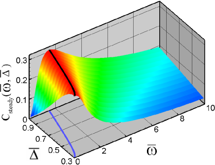
Figure 3: Plot of the $T=0$ steady state concurrence (cf. Eq. (34)) as a function of the scaled energy $\bar{\omega}$ and the scaled anisotropy parameter $\bar{\Delta}$ (ranging from $0.309$ to $1$), where $\bar{\omega}=\omega/\gamma$ and $\bar{\Delta}=\Delta/\gamma$. The solid lines locate the maximum value of concurrence (cf. Eq. (36)); see text for discussion.

4 Temperature Dependence of the Steady State Concurrence

It is of interest to examine how the steady state entanglement obtained for zero temperature in the prior section changes when the temperature is finite. For simplicity, we assume that each qubit interacts with the same thermal bath. It is known that the equilibrium entanglement must vanish at some finite temperature [34]. In order to examine the effect of thermal decoherence on the entanglement for our system we consider the following master equation [35, 36]:

$$\dot{\rho} = -i\left[H,\rho\right]+\gamma{(\bar{n}+1)}{\cal D}\left[S_{1}^{-}\right]\rho+\gamma{(\bar{n}+1)}{\cal D}\left[S_{2}^{-}\right]\rho$$ (37)

$$+\gamma\bar{n}{\cal D}\left[S_{1}^{+}\right]\rho+\gamma\bar{n}{\cal D}\left[S_{2}^{+}\right]\rho,$$

where $\bar{n}$, the average excitation of the thermal bath, parametrizes the temperature. Note that $\bar{n}$ is zero at zero temperature, whereupon one observes that Eq. (37) reduces to Eq. (3); also, $\bar{n}$ becomes infinite as the temperature becomes infinite. The master equation (37) may be solved to obtain the following analytic expressions for the steady state density matrix of our system:

$$\rho_{11} = \frac{\bar{n}^{2}(4\bar{\omega}^{2}+(1+2\bar{n})^{2})+\bar{\Delta}^{2}(1+2\bar{n})^{2}}{(1+2\bar{n})^{2}(4\bar{\omega}^{2}+(1+2\bar{n})^{2}+4\bar{\Delta}^{2})}$$

$$\rho_{22} = \rho_{33}=\frac{1}{4}[1-\frac{4\bar{\omega}^{2}+(1+2\bar{n})^{2}}{(1+2\bar{n})^{2}(4\bar{\omega}^{2}+(1+2\bar{n})^{2}+4\bar{\Delta}^{2})}]$$

$$\rho_{44} = \frac{4\bar{\omega}^{2}(1+\bar{n})^{2}+(1+2\bar{n})^{2}((1+\bar{n})^{2}+\bar{\Delta}^{2})}{(1+2\bar{n})^{2}(4\bar{\omega}^{2}+(1+2\bar{n})^{2}+4\bar{\Delta}^{2})}$$

$$\rho_{14} = -\frac{\bar{\Delta}(2\bar{\omega}+i(2\bar{n}+1))}{(1+2\bar{n})(4\bar{\omega}^{2}+(1+2\bar{n})^{2}+4\bar{\Delta}^{2})}$$ (38)

In the limit of zero temperature (i.e., $\bar{n}\rightarrow 0$), the density matrix elements in Eq. (4) reduce to the results in Eqs. (30) - (33). In the limit of infinite temperature (i.e., $\bar{n}\rightarrow\infty$), the density matrix becomes diagonal, with each diagonal element equal to $1/4$, indicating, as expected [34], that all entanglement vanishes.

The concurrence may be calculated for the finite temperature, steady-state density matrix in Eq. (4) to obtain:

$$C(\bar{\omega},\bar{\Delta},\bar{n}) = 2\frac{\sqrt{\bar{\Delta}^{2}(4\bar{\omega}^{2}+(1+2\bar{n})^{2})}}{(1+2\bar{n})(4\bar{\Omega}^{2}+(1+2\bar{n})^{2})}-\frac{1}{2}$$ (39)

$$+\frac{(4\bar{\omega}^{2}+(1+2\bar{n})^{2})}{2[(1+2\bar{n})^{2}(4\bar{\Omega}^{2}+(1+2\bar{n})^{2})]},$$

where all system parameters have been normalized by the relaxation rate $\gamma$: $\bar{\Delta}=\Delta/\gamma$, $\bar{\omega}=\omega/\gamma$, and $\bar{\Omega}=\Omega/\gamma=\sqrt{\bar{\omega}^{2}+\bar{\Delta}^{2}}$ (cf. Eq. (19)). In the limit of zero temperature (i.e., $\bar{n}\rightarrow 0$), the concurrence in Eq. (39) reduces to that in Eq. (34). The behavior of this finite temperature, steady state concurrence is shown in Fig. 4 for the same two sets of system parameters considered in Figs. 1 and 2 respectively. One sees that both curves decrease with increasing $\bar{n}$ until eventually the concurrence vanishes at a finite value of $\bar{n}$, as expected [34]. One sees also that the larger the value of the interaction asymmetry parameter $\bar{\Delta}$, the larger the value of the concurrence at any finite value of $\bar{n}$. For any fixed temperature (i.e., $\bar{n}$), as the effective magnetic field, $\bar{\omega}$, increases, the concurrence takes a finite, non-zero value. In the limit $\bar{\omega}\rightarrow\infty$, one has that $\bar{n}\rightarrow 0$ and $C\rightarrow|\bar{\Delta}|/\bar{\omega}$. This decrease with $\bar{\omega}^{-1}$ as well as the fact that $C\geq 0$ only if $\bar{\Delta}\not=0$ is consistent with the results of Ref. [4].

Figure 4: Plots of the finite temperature, steady state concurrence (cf. Eq. (39)) as a function of the average thermal excitation function, $\bar{n}$, for the same two sets of system parameters as in Figs. 1 and 2. The curve in the lower left corner of the figure corresponds to the same system parameters as in Fig. 1; the curve close to the diagonal corresponds to the same system parameters as in Fig. 2. Note that at $\bar{n}=0$ both curves begin at the steady state values of the concurrence shown in Figs. 1 and 2.

5 Discussion and Conclusions

Quantum coherence is a necessary requirement for the existence of entanglement. One may define coherence existing in a single qubit as “local coherence” while coherence between two qubits $A$ and $B$ may be defined as “global coherence” [23]. How do local and global coherence relate to entanglement? The answer for our model system may be understood by considering the relation between a general two-qubit density matrix, $\rho_{AB}$, and the reduced density matrices, $\rho^{A}$ and $\rho^{B}$, for each of the two qubits, where $\rho^{A}=tr_{B}(\rho^{AB})$ is obtained by tracing over the degrees of freedom of qubit $B$, and similarly for $\rho^{B}$. In our model, after doing partial traces, we find that in the steady state the local coherence of each qubit is zero, i.e., $\rho^{A}$ and $\rho^{B}$ are diagonal matrices. However, there exist global coherence terms for our system (i.e., $\rho_{14}$ and $\rho_{41}$) that are non-zero, indicating that global, not local, coherence is responsible for this system’s entanglement. For time $t>0$, $\rho_{14}$ and $\rho_{41}$ for our system are always non-zero; $\rho_{23}$ and $\rho_{32}$ may be non-zero for finite times, but vanish in the steady state. Ref. [23] considered a decohering system of two entangled (but non-interacting) qubits. In that system, both local and global coherence vanished in the asymptotic time limit; however, in some cases, the latter vanished for finite times [23].

An interesting question regarding the steady state of our model system is whether or not it is a decoherence-free subspace [37]. Typically, a decoherence-free subspace is defined to be one for which the decoherence terms in the system’s master equation vanish [38]. For our system, this would mean that the second and third terms on the right of Eq. (3) vanish for the case of zero temperature or, for the case of finite temperature, that all terms except for the first one on the right of Eq. (37) vanish. However, in our system, the decoherence terms in Eqs. (3) and (37) do not vanish; rather the sum of all terms on the right hand sides of these two master equations vanish. This implies that population relaxation and thermal decoherence (in the case of finite temperature) are competing with the spin-spin interaction terms to create a steady state level of entanglement, as measured by the concurrence.

We note, finally, that a somewhat different model system studied by S. Montangero, G. Benenti, and R. Fazio [39] has found results for the pairwise concurrence that are somewhat similar to those we find for our system. Specifically, they have considered the entanglement of a pair of spins within a qubit lattice in which there is disorder in the spin-spin couplings. They have identified a regime in which the pairwise concurrence is stable against such disorder in the couplings and has a value in the range of 0.2-0.3 [39]. We note that the numerical maximum for their “saturation value” of the concurrence is quite close to the analytical maximum we have derived in this paper (cf. Eq. (36)). It is interesting to observe that our analytic result for the maximum value of the steady state concurrence is constant for a range of system parameters (cf. Eqs. (35)-(36)). Whether or not this analytical maximum holds also for other systems, such as the different one considered in [39], is an open question.

In summary, we have provided a detailed analytical and numerical analysis of decoherence for an interacting two-qubit model system having a Hamiltonian identical in form to that for the well-known two-qubit Heisenberg XY spin 1/2 system in the presence of an (effective) external uniform magnetic field. For $T=0$, we have presented an analytic solution for the evolution of entanglement, measured by concurrence, for the case that both qubits are initially in their ground states; we have presented also numerical solutions for two other typical initial states. We find that our system is robust against decoherence: a steady state level of entanglement, controllable by the values of the system parameters, is always reached for zero or finite, low temperatures. For the $T=0$ case, we have defined this steady state analytically and obtained the parameter values that maximize its entanglement. For $T>0$, the steady state level of entanglement is found to vanish at a finite temperature. Since our model interaction Hamiltonian describes also mesoscopic objects that interact via their spins (e.g., cf. Ref. [40]), it may be that a certain level of entanglement is robust against decohering interactions with an environment even for such objects. As noted by Ghosh et al. [41], even “the slightest degree of entanglement can have profound effects” on the properties of mesoscopic spin systems.

We acknowledge stimulating discussions with Joseph H. Eberly, Hong Gao, Andrei Y. Istomin, Murray Holland, Ting Yu, and Peter Zoller. This work is supported in part by grants from the Nebraska Research Initiative and the W. M. Keck Foundation.

References

References

- [1] 2000 The Physics of Quantum Information, edited by Bouwmeester D, Ekert A, and Zeilinger A (Berlin:Springer)
- [2] Arnesen M C, Bose S, and Vedral V 2001 Phys. Rev. Lett. 87 017901
- [3] Wang X 2001 Phys. Rev. A 64 012313
- [4] Lagmago Kamta G and Starace A F 2002 Phys. Rev. Lett. 88 107901
- [5] Korepin V E, Bogoliubov N M, and Izergin A G 1993 Quantum Inverse Scattering Method and Correlation Functions (Cambridge: Cambridge University Press) pp. 63-79
- [6] Loss D and DiVincenzo D P 1998 Phys. Rev. A 57 120
- [7] Burkard G, Loss D, and DiVincenzo D P 1999 Phys. Rev. B 59 2070
- [8] Imamoḡlu A et al. 1999 Phys. Rev. Lett. 83 4204
- [9] Ernst R R, Bodenhausen G, and Wokaun A 1988 Principles of Nuclear Magnetic Resonance in One and Two Dimensions (Oxford: Clarendon Press)
- [10] Nielson M A and Chuang I L 2000 Quantum Computation and Quantum Information (Cambridge: Cambridge University Press).
- [11] Sørensen A and Mølmer K 1999 Phys. Rev. Lett. 83 2274
- [12] Duan L-M, Demler E, and Lukin M D 2003 Phys. Rev. Lett. 91 090402
- [13] Georgeot B and Shepelyansky D L 2000 Phys. Rev. E 62 3504; 2000 ibid. 62 6366
- [14] Makhlin Y, Schön G, and Shnirman A 2001 Rev. Mod. Phys. 73 357, Appendix A
- [15] Bloch F 1946 Phys. Rev. 70 460
- [16] Zurek W H 1991 Phys. Today 44(10) 36; 1993 Prog. Theor. Phys. 89 281; 2003 Rev. Mod. Phys. 75 715
- [17] Albrecht A 1992 Phys. Rev. D 46 5504
- [18] de Sousa R and Das Sarma S 2003 Phys. Rev. B 68 115322; Hu X, de Sousa R, and Das Sarma S 2001 arXiv:cond-mat/0108339.
- [19] Dodd P J and Halliwell J J 2004 Phys. Rev. A 69 052105
- [20] Viola L, Lloyd S, and Knill E 1999 Phys. Rev. Lett. 83 4888
- [21] Beige A, Braun D, Tregenna B, and Knight P L 2000 Phys Rev. Lett. 85 1762
- [22] Braun D, Haake F, and Strunz W T 2001 Phys. Rev. Lett. 86 2913
- [23] Yu T and Eberly J H 2004 Phys. Rev. Lett. 93 140404
- [24] Bennett C H, DiVincenzo D P, Smolin J A, and Wootters W K 1996 Phys. Rev. A 54 3824
- [25] Hill S and Wootters W K 1997 Phys. Rev. Lett. 78 5022; Wootters W K 1998 Phys. Rev. Lett. 80 2245
- [26] Carmichael H J 1999 Statistical Methods in Quantum Optics 1:Master Equations and Fokker-Planck Equations (Berlin:Springer-Verlag) p. 16
- [27] Gardiner C W and Zoller P 2000 Quantum Noise, 2nd Ed. (Berlin: Springer-Verlag) p. 147
- [28] Lindblad G 1976 Commun. Math. Phys. 48 199
- [29] Vedral V, Plenio M B, Rippin M A, and Knight P L 1997 Phys. Rev. Lett. 78 2275
- [30] Horodecki M, Horodecki P, and Horodecki R 1998 Phys. Rev. Lett. 80 5239
- [31] Rains E M 1999 Phys Rev. A 60 173; 60 179
- [32] Preskill J Lecture Notes on Quantum Information and Quantum Computation at www.theory.caltech.edu/people/preskill/ph229
- [33] Zoller P 2005 private communication
- [34] Fine B V, Mintert F, and Buchleitner A 2005 Phys. Rev. B 71 153105
- [35] See Ref. [26], Eq. (2.26)
- [36] Mintert F, Carvalho A R R, Kuś M, and Buchleitner A 2005 quant-ph/0505162v1, Eq. (110)
- [37] See, e.g., p.498 of Ref. [10].
- [38] Lidar D A, Chuang I L, and Whaley K B 1998 Phys. Rev. Lett. 81 2594
- [39] Montangero S, Benenti G, and Fazio R 2003 Phys. Rev. Lett. 91 187901
- [40] Skomski R, Istomin A Y, Starace A F, and Sellmyer D J 2004 Phys. Rev. A 70 062307
- [41] Ghosh S, Rosenbaum T F, Aeppli G, and Coppersmith S N 2003 Nature 425 48