One- and two-dimensional quantum walks in arrays of optical traps

Abstract

We propose a novel implementation of discrete time quantum walks for a neutral atom in an array of optical microtraps or an optical lattice. We analyze a one-dimensional walk in position space, with the coin, the additional qubit degree of freedom that controls the displacement of the quantum walker, implemented as a spatially delocalized qubit, i.e., the coin is also encoded in position space. We analyze the dependence of the quantum walk on temperature and experimental imperfections as shaking in the trap positions. Finally, combining a spatially delocalized qubit and a hyperfine qubit, we also give a scheme to realize a quantum walk on a two-dimensional square lattice with the possibility of implementing different coin operators.

PACS numbers: 03.67.-a, 32.80.Pj, 42.50.-p

I Introduction

In classical computation, random walks are powerful tools to address a large number of problems in many areas of science, as, for example, graph-connectivity or satisfiability problems class_alg . It is this success of random walks that motivated to study their quantum analogues in order to explore whether they might extend the set of quantum algorithms. Two distinct types of quantum walks have been identified: for the continuous time quantum walk a time-independent Hamiltonian governs a continuous evolution of single particle in a Hilbert space spanned by the vertices of a graph contQWalks , while the discrete time quantum walk requires a quantum coin as an additional degree of freedom in order to allow for a discrete time unitary evolution in the space of the nodes of a graph. The connection between both types of quantum walks is not clear up to now KempeReview , but in both cases different topologies of the underlying graph have been studied, e.g., discrete time quantum walks on circles QWinCircle , on an infinite line QWonLine , on more-dimensional regular grids QWmoreDim , and on hypercubes QWonHC . The field has recently been reviewed by Kempe KempeReview .

Several algorithms based on quantum walks have been proposed qw_algo ; qw_algo2 ; qw_algo3 ; coinsfaster . To implement such an algorithm in a physical system it ultimately has to be broken down into a series of gates acting on a register of qubits KempeReview . From the more fundamental point of view however more straight-forward implementations are interesting, i.e., direct implementations of a quantum walker (a particle, a photon etc.) moving, e.g., in position or momentum space. So far some setups for one-dimensional realizations have been analyzed, including trapped ions QWIonTrap , neutral atoms in optical lattices with state dependent potentials QWOptLat , single-photon sources together with linear optical elements QWLOE , and also with classical optics knight . Here we use the idea of spatially delocalized qubits (SDQ) developed in PRLJordi to propose a novel quantum walk implementation with neutral atoms. The particle is walking in position space, but in contrast to the proposal in QWOptLat also the quantum coin is represented by a spatial degree of freedom, as it is implemented by the presence of the atom in the ground state of one out of two trapping potentials. The particle is manipulated only by varying the trapping potentials, which induces tunneling between traps, and no state dependent potentials are necessary. This concept can be applied to neutral atoms trapped in optical lattices opt_lat , in magnetic potentials mag_pot , as well as in arrays of microtraps PRLBirkl ; here we will especially analyze the latter case. We will also show how a combination of a spatially delocalized qubit and a hyperfine qubit together with state dependent potentials allows to implement a quantum walk on a two-dimensional square lattice. Quantum walks in higher dimensions offer a very rich structure of dynamics, and recently a spatial search algorithm using a modified quantum walk on a two-dimensional grid has been proposed coinsfaster .

For the one-dimensional case we will discuss the influence of non-adiabatic processes and of shaking of the trap positions, and we will estimate the effect of decoherence. We will also consider dependencies of the quantum walk on the vibrational trapping state and thus on the temperature and show that, within a range of parameters accessible in experiments, a transition from the quantum walk to the classical random walk can be studied. This is not only interesting from a fundamental point but also allows to assess the degree of control that can be reached in the experiment.

It has been noted classical ; knight ; classical2d , that essentially only interference is necessary for a quantum walk, such that it can be implemented with classical fields. Nevertheless considering setups with neutral atoms is justified by a strong interest in these systems as tools for quantum computation qc , as well as by the possibility to include further effects as, e.g., quantum walks with two or more (possibly interacting) particles yasser .

II Quantum walks and optical microtraps

II.0.1 Quantum walks

Let a particle move on a one-dimensional infinite line, such that it can only hop between discrete sites $x=k\cdot a$ labeled by $k\in\{\ldots,-2,-1,0,1,2,\ldots\}$, with $a$ being the distance between sites. At each time step the particle moves with equal probability to either of the adjacent sites. For a classical random walk, the probability for the particle to be at a certain site for a large number of steps approaches a gaussian function centered around its initial position $x_{0}$, with the variance $\sigma^{2}=\langle(x-x_{0})^{2}\rangle$ growing linearly with the number of steps $n$. For the quantum version a state $|k\rangle$ is attached to each site $x=k\cdot a$, i.e., the particle is walking in $\mathcal{H}_{W}=\text{span}\left\{|k\rangle,k=\ldots,-2,-1,0,1,2,\ldots\right\}$. However, the random move cannot be just replaced by walking to the left and to the right in superposition, as this turns out to be non-unitary meyer . For this reason a quantum coin is introduced as an additional degree of freedom. In the simplest case of the quantum walk on a line, the coin space $\mathcal{H}_{C}$ is two-dimensional and we will denote the states that span $\mathcal{H}_{C}$ by $|-\rangle$ and $|+\rangle$, and the total Hilbert space is thus $\mathcal{H}_{W}\otimes\mathcal{H}_{C}$. Each step of the quantum walk is then composed from two operations: (i) applying a unitary operation $C$ to the coin (simultaneously at all sites), e.g., a Hadamard operation $C=\textrm{{H}}$:

$$(\mathbb{I}\otimes\textrm{{H}})|k,\pm\rangle=\frac{1}{\sqrt{2}}(|k,+\rangle\pm|k,-\rangle)\quad\forall k,$$ (1)

followed by (ii) applying a displacement operation $O_{\text{1D}}$ which moves the particle left or right depending on the coin:

$$O_{\text{1D}}|k,\pm\rangle=|k\pm 1,\pm\rangle\quad\forall k,$$ (2)

where we have not explicitly written the tensor product: $|k\rangle\otimes|\pm\rangle\equiv|k,\pm\rangle$ etc. The probability distribution arising from the iterated application of $W=O_{\text{1D}}(\mathbb{I}\otimes\textrm{{H}})$ is, except for the first three steps, significantly different from the distribution of the classical walk: if the coin initially is in a suitable superposition of $|-\rangle$ and $|+\rangle$ it has two maxima symmetrically displaced from the starting point. In general the exact form of the distribution, especially the relative height of the maxima, depends on the initial coin state. Compared to the classical random walk its quantum version propagates faster along the line: its variance grows quadratically with the number of steps $n$, $\sigma^{2}\propto n^{2}$, compared to $\sigma^{2}\propto n$ for the classical random walk.

For the walk on a line, H is, up to phases (which can be absorbed also into the initial state), the only unbiased coin operator coinsandstates . For a two-dimensional regular square lattice a much richer structure of coin operators and possible probability distributions arises. As has been observed by Mackay et al. QWmoreDim and by Tregenna et al. coinsandstates in this case different unbiased coin operators and initial states can be chosen that produce significantly different dynamics, ranging from distributions with a sharp centered spike to distributions having the shape of a ring.

II.0.2 Optical microtraps

As a particular setup for the implementation, we consider the controlled motion of neutral atoms in arrays of optical microtraps. The microtraps are created by illuminating a set of microlenses with a red detuned laser beam, such that in each of the foci of the individual lenses neutral atoms can be stored by the dipole force PRLBirkl . By illuminating the set of microlenses by two independent laser beams, it is possible to generate two sets of traps which can be approached or separated by changing the angle between the two lasers. This allows the atom to propagate between different microtraps. The optical potentials have a gaussian shape, i.e.,

$$V(x)=-V_{0}\exp\left({-\frac{1}{2V_{0}}m\omega_{x}^{2}x^{2}}\right)=-V_{0}\exp\left({-\frac{\hbar\omega_{x}}{2V_{0}}(\alpha x)^{2}}\right).$$ (3)

For the simulations we present here, we will use $V_{0}=200\;\hbar\omega_{x}$. In this case the traps are deep enough to be described by harmonic potentials of frequency $\omega_{x}$ in the limit of large separation. Then $\alpha^{-1}=\sqrt{\hbar/m\omega_{x}}$ denotes the spread of the ground state in position space, with $m$ being the mass of the atom.

For the preparation of the initial state we assume that a single atom can be placed in the ground state of a specific trap. For this reason, and also to be able to read out the final state of the system, it is necessary to be able to address each trap separately. This addressability has already been demonstrated in arrays of up to $10\times 10$ microtraps PRLBirkl .

III One-dimensional walks

The implementation of the coin at each site $k$ will follow the idea of spatially delocalized qubits from PRLJordi , i.e., the basis states $|k,\pm\rangle$ will be represented by a single atom occupying the ground state of one of two adjacent traps. Unitary operations are performed by approaching the two traps forming the coin, allowing the atom to tunnel between them. In the following we will use quantum optics notation to describe the effect of tunneling between traps, e.g., an operation exchanging the population of two traps will be termed $\pi$ pulse and a Hadamard-like operation $|k,\pm\rangle\mapsto\frac{1}{\sqrt{2}}(|k,+\rangle\pm i|k,-\rangle)$ will be termed $\pi/2$ pulse PRLJordi .

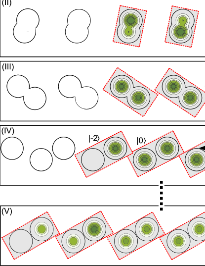
Figure 1: (Color online) Configuration with two rows of traps, the qubit is implemented ’perpendicular’ to the rows (dashed rectangles show which two traps form each qubit). The upper (lower) row moves left (right) with constant velocity (see arrows on right). (I) After the first step: $|\psi\rangle=1/\sqrt{2}(|-1,-\rangle+|+1,+\rangle)$; (II)-(III) the coin operation, in this case a Hadamard gate, is performed when the traps pass each other; (IV) the shift $O_{1D}$ is implicit through a redefinition of the qubits. After an even (odd) number of shift operations only the even (odd) qubits (compared to the standard quantum walk definition) are defined; (V) the probability distribution after the sixth displacement operation. For the numerical simulation we used a potential which, along the line connecting the centers of two traps, reads $V(x)=\hbar\omega_{x}\min\left\{\alpha^{2}(x-a)^{2},\alpha^{2}(x+a)^{2}\right\}$. The velocity is chosen such that during the passing of two traps a Hadamard operation is performed. The initial state is $|\psi_{\text{init}}\rangle=\frac{1}{\sqrt{2}}\left(|0,-\rangle+|0,+\rangle\right)$.

We propose two closely related configurations, both leading to a quantum walk. For the first configuration two rows of traps are necessary. Each coin is defined through one trap from each row. By moving both rows in opposite directions with appropriately chosen distance and velocity, the coin operations are performed when the traps pass each other at close distance. The displacement is implicit through a redefinition of the coin each time two traps have passed. Fig. 1 shows the first steps in the temporal evolution of the configuration with two rows of traps along with the corresponding probability distributions resulting from an integration of the two-dimensional Schrödinger equation (see figure caption for details). Fig. 1 (I–III) show the coin operation, (III-IV) the redefinition of the coins and (V) shows the probability distribution after the sixth displacement operation. The onset of the quantum walk character of the distribution is clearly visible as two maxima symmetrically displaced from the origin appear. If the continuous displacement of one row with respect to each other requires mechanical movement of an array of lenses this setup is quite challenging, a problem which might be overcome by using holographic techniques to generate arrays of microtraps bargamini .

In what follows we will concentrate on the coin being implemented ’parallel’ to the direction of displacement, such that only a single line of traps is necessary, see Fig. 2. Labeling the traps of the $k$th qubit by $2k$ and $2k+1$, for coin operations the traps $2k$ and $2k+1$ are approached, while for the steps in the walk a $\pi$-pulse between traps in adjacent qubits, i.e., between traps $2k+1$ and $2(k+1)$, moves the atom one step to the left or to the right, respectively. Contrary to the displacement operator from Eq. (2), this procedure flips the coin operator at each move, i.e., we have $O_{\text{1D}}|k,\pm\rangle=|k\pm 1,\mp\rangle$ (termed flip-flop walk in coinsfaster ). Clearly the experimental requirement is to be able to move all odd (or all even) traps as a whole to both directions, thus approaching each second trap to its left or right neighbor. This can be realized as described in section II.0.2 in optical microtraps PRLBirkl , but also in optical lattices vibrational ; weitz1 or magnetic microtraps mag_pot .

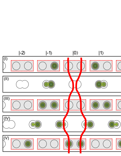
Figure 2: (Color online) Configuration with one row of traps, the qubit is implemented ’parallel’ to the rows (grey boxes). (I) After the first step: $|\psi\rangle=(|-1,+\rangle+|+1,-\rangle)/\sqrt{2}$; (II) traps inside each qubit are approached to give the coin operation; (IV) the shift $O_{\text{1D}}$ is realized through approaching traps of adjacent qubits.

For the gaussian trapping potentials of Eq. (3), Fig. 3 (i) shows a simulation of the quantum walk for potential depth $V_{0}=200\;\hbar\omega_{x}$ and an initial separation $\alpha a_{\text{max}}=60$, obtained from an integration of the one-dimensional Schrödinger equation using Fourier transformation and a split-step method. Initially the atom is prepared in an equal superposition of the two ground states of the central qubit, i.e., of the two central traps, such that $|\psi_{\text{init}}\rangle=\frac{1}{\sqrt{2}}(|0,+\rangle+|0,-\rangle)$. The distance of the traps is changed between the maximal value $\alpha a_{\text{max}}=60$ and a minimal value $\alpha a_{\text{min}}=28.8$. The latter distance is for the given trapping parameters close enough for tunneling to take place. Moving the traps adiabatically between this distances requires techniques to optimize the moving process while suppressing transitions between motional states optimization . In this way, the time $t_{r}$ necessary to approach – or separate – the traps can be reduced to $\omega_{x}t_{r}=100$ or below while maintaining a fidelity larger than $F=0.999$ PRLJordi . The time $t_{i}$ for which the traps are kept at the distance $a_{\text{min}}$ is chosen such that alternately a $\pi$ pulse and a $\pi/2$ pulse are applied. The figure shows the population of the traps after $t=10,\,20$, and $25$ steps. In Fig. 3 (i) the characteristic shapes of the quantum walk distributions are visible. Subsequently we will analyse how the probability distribution changes if different vibrational states are involved or experimental imperfections are present.

III.0.1 Excited vibrational states: the influence of temperature

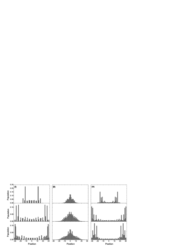
Figure 3: The probability distribution to find the atom at a specific trap site, with (I) the ground state and (II) the first excited state as the initial vibrational state, for a one-dimensional quantum walk on a finite line of 62 traps; from top to bottom distributions after $t=10$, $20$, and $30$ steps are shown. Parameters: $V_{0}=200\hbar\omega_{x}$, $\alpha a_{\text{max}}=60$, $\alpha a_{\text{min}}=28.8$, and $\omega_{x}t_{r}=100$; $\omega_{x}t_{i,\pi}=20.25$ for the $\pi$ pulse and $\omega_{x}t_{i,\pi/2}=112$ for the $\pi/2$ pulse (for simplicity we fixed $a_{\text{min}}$ and then searched for the smallest $t_{i}$ that produces the desired operation. As tunneling already happens for $a>a_{\text{min}}$, $t_{i}=0$ does not give the identity operation, and for this reason $t_{i,\pi/2}>t_{i,\pi}$). (III) like (II), but with $\omega_{x}t_{r}=200$, such that non-adiabatic excitations are suppressed.

Tunneling as well as adiabaticity do crucially depend on the timing of the change of the trap separation. For all simulations $t_{r}$, the time needed to move the traps together or apart, and $t_{i}$, the time for which the trap separation is kept constant, are chosen to apply the correct operations for the vibrational ground state. If the atom starts in an excited vibrational state, then the tunneling rate is larger and thus in general the coin operator $C$ as well as the displacement operator $O_{\text{1D}}$ change. The former will be distinct from the Hadamard operator H and in general biased,

$$C^{\prime}|k,\pm\rangle=\sqrt{p}|k,+\rangle\pm\sqrt{1-p}\;e^{i\Delta_{C}}|k,-\rangle,$$ (4)

(the standard unbiased Hadamard operator has $p=\frac{1}{2}$ and $\Delta_{C}=0$), the latter will take a general form

$$O^{\prime}_{\text{1D}}|k,\pm\rangle=\sqrt{c}|k\pm 1,\mp\rangle\pm\sqrt{1-c}\;e^{i\Delta_{O}}|k,\pm\rangle.$$ (5)

($c=1$ and $\Delta_{O}=0$ for the standard displacement operator). For an atom in a fixed vibrational level, $p,\,\Delta_{C},\,c$ and $\Delta_{O}$, and thus the operators $C^{\prime}$ and $O^{\prime}_{1D}$ are constant, because the movement of traps is assumed to be unchanged throughout the process. In such a case the qualitative shape of the probability distribution is not modified significantly, it still shows the characteristic symmetrically displaced peaks. However, a simulation for an atom initially in the first excited vibrational state, c.f., Fig. 3 (ii), shows a distribution which essentially has a central peak and long symmetric tails. In this case the variance $\sigma^{2}$ grows only linearly with the number of steps, as compared to a quadratic increase of the variance for the ground state distribution. The difference to the expected result can be attributed to the fact that the approaching and separating processes were optimized to suppress non-adiabatic excitations from the ground state. For higher vibrational states excitations are non-negligible, causing coin as well as displacement operator to induce transitions between different trapping states. Then effectively we have a one-dimensional walk with a higher dimensional coin. A quantum walk distribution should be reobtained when restricting the quantum walk to some fixed vibrational state by suppressing non-adiabatic transitions. This can be done by increasing the time $t_{r}$ used to approach the traps. Then, as can be seen in Fig. 3 (iii), again the characteristic displaced peaks of the quantum walk probability distribution appear. As for the ground state, the variance increases quadratically with the number of steps. Note however that the distribution is not the same as for the ground state due to different coin and displacement operators.

A more realistic assumption than starting from a pure state with the atom being in a specific vibrational level is to consider a thermal Boltzmann distribution of the vibrational modes

$$\rho=\frac{1}{z}\sum_{j=0}^{\infty}e^{-\beta E_{j}}|j\rangle\langle j|,\ \ z=\sum_{j}^{\infty}e^{-\beta E_{j}},\ \ \beta=\frac{1}{k_{B}T},$$ (6)

where $E_{j}$ is the energy of the $j$th vibrational mode. In this case the experimentally accessible probability distributions are the classically averaged probability distributions, weighted with factors $\exp(-\beta E_{J})/z$. Respective probability distributions after $n=20$ steps are shown in Fig. 4 for initial ground state populations of $50$% and $25$%, corresponding to a mean number of vibrational quanta of $\langle\nu\rangle=1$ and $\langle\nu\rangle=3$, or to a temperature of $T=1.1\;\mu$K and $T=2.7\;\mu$K (for Rb atoms and trap frequency $\omega_{x}=10^{5}$ s^-1), respectively. The characteristics of the quantum walk remain visible even at such $\langle\nu\rangle$. In optical lattices with parameters similar to what we consider here, ground state populations of above $98$% have been achieved jessen . Thus we can expect that the range of temperatures necessary to observe the quantum distribution is well within the reach of experiments.

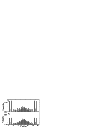
Figure 4: Probability distributions after $t=20$ steps for thermal Boltzmann distributions of vibrational modes, initial ground state population (I) $50$% and (II) $25$%. All other parameters as in Fig. 3.

III.0.2 Experimental imperfections and decoherence

As an important experimental imperfection we will analyze shaking of the centers of the traps. We assume that the movement of traps in the even or odd sets (traps $2k$ or $2k+1$, respectively) is correlated. For an implementation with optical microtraps this is justified, because each set can be generated from a single laser beam, as described in section II.0.2, but it will also describe the situation for optical lattices with tunneling controlled by changing the intensity of one out of two counterpropagating laser beams, as in vibrational ; weitz1 . We also anticipate shaking with a fixed frequency far away from the trapping frequency. This will not eliminate transitions between vibrational states, as it alters the (optimized) path to approach the traps. Due to the strong sensitivity of tunneling on the distance, shaking will give rise to changes in the rate of the population oscillation between the traps, i.e., coin and displacement operators will change. They will even be different from step to step, as shaking is not correlated to the global motion of approaching the traps. The consequences of this random variation should be similar to the effects observed in the presence of decoherence. Decoherence in quantum walks has been studied by Kendon and Tregenna in a general framework QWdecoh and by Dür et al. for the special case of an optical lattice implementation of a quantum walk QWOptLat . In the presence of decoherence, the probability distribution of the quantum walk on the (infinite) line ultimately collapses to the gaussian distribution characteristic for the classical random walk. However, for the product of the number of steps $t$ and the decoherence rate $p$ being small enough, decoherence does not significantly degrade the quadratic spreading of the walk. As has furthermore been found in QWdecoh , for a certain intermediate choice of $tp$ a highly uniform distribution of the probabilities between positions $\pm t/\sqrt{2}$ can be observed if decoherence acts on the position degree of freedom or on both, the coin and the position degree of freedom; note that for our implementation the effect of shaking corresponds to the latter case.

In Fig. 5 the results for a sinusoidal variation of the trap distances around the perfect value with frequency $\omega_{\text{Shake}}=0.01\;\omega_{x}$ and amplitude $\alpha\Delta a$ are shown. The transition from the quantum to a classical distribution takes place for amplitudes on the order of a percent of the minimal distance, the intermediate flat distribution is clearly visible at $\alpha\Delta a\approx 0.09$. For larger amplitudes of shaking the non-adiabatic transitions are dominant (Fig. 5 (II)), and the variance decreases strongly with increasing shaking (Fig. 5 (III)). For smaller amplitudes however the variance initially increases with increasing amplitude of shaking. To quantify the flatness of the distribution we also calculate the total variational distance $\nu(t)=\sum_{n}|P(n,t)-P_{u}(t)|$ to the uniform distribution $P_{u}(t)$ of half width $t/\sqrt{2}$ QWdecoh . Here $P(n,t)$ is the probability to find the particle in the traps belonging to the $n$-th qubit after $t$ steps. As Fig. 5 (IV) shows, the total variational distance decreases initially, before it increases again as the probability distribution approaches a gaussian.

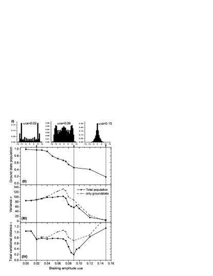
Figure 5: The effect of shaking of the trap position on the quantum walk. Shaking is modeled by a sinusoidal variation of the trap distances around the perfect value, with frequency $\omega_{Shake}=0.01\omega_{x}$ and amplitude $\alpha\Delta a$ (all the other parameters are as in Fig. 3). (I) The probability distributions for various values of $\alpha\Delta a$ (after tracing over the coin degree of freedom). (II) Ground state population, (III) variance, and (IV) variational distance $\nu$ from the uniform distribution after $t=17$ steps. In (II) and (III) dashed lines and squares give the respective values for the full population, dotted lines and circles for the ground state only.

Let us discuss the duration of the operations necessary for the quantum walk in order to estimate the influence of other decoherence mechanisms in the experiment. As the processes rely on tunneling, the duration of a single operation is on the order of the inverse trapping frequency, which typically is about $\omega_{x}=10^{5}$ s^-1 PRLBirkl ; BirklOC . For the parameters used here a single application of $O_{\text{1D}}\;(\mathbb{I}\otimes C)$ takes around $5$ ms. The dominant decoherence mechanism can be expected to be the scattering of photons from the trapping laser, with scattering rates on the order of $0.1\ldots 1$ s^-1 PRLBirkl ; BirklOC . Then the probability for a decoherence event to occur within a single step is $p=0.0005\ldots 0.005$ and for $t=17$ applications of $O_{\text{1D}}\;(\mathbb{I}\otimes C)$ we have $tp=0.0085\ldots 0.085$. For optical lattices the same decoherence mechanism is present, but also decoherence through fluctuations in the phase of the lasers producing the lattice, giving rise to fluctuations in the trapping potentials should be taken into account. One the other hand operations can be an order of magnitude faster, as the initial separation of the atoms can be made shorter, such that decoherence rates similar to the case of optical microtraps can be expected. In both cases these decoherence mechanisms affect the coin as well as the position, and for this case the crossover from the quantum to the classical distribution has been numerically estimated in QWdecoh to take place at $tp\approx 2.6$. For this reason it should be possible to observe the quantum walk in such systems and to analyze changes caused by temperature and shaking without being limited by decoherence from photon scattering etc. The strong dependence on temperature and on non-adiabatic transitions of the quantum walk with delocalized qubits might thus be interesting as a tool to analyze to which extent the ground state population, the shaping of the trapping potentials, and tunneling processes can be controlled for a particular experimental setup. In addition, quantum walks in this particular physical system could be used to investigate how decoherence acts with respect to the spatial degree of freedom.

IV A two-dimensional quantum walk

For the two-dimensional quantum walk on a regular square lattice, i.e., if

$$\mathcal{H}_{W}=\text{span}\left\{|(k,l)\rangle,k\,\;\text{and}\,\;l\in\{\ldots,-2,-1,0,1,2,\ldots\}\right\},$$

a four dimensional coin degree of freedom to control the displacement of the particle into the four possible directions is necessary:

$$\mathcal{H}_{C} = \text{span}\left\{|++\rangle\equiv|\nearrow\rangle,|-+\rangle\equiv|\nwarrow\rangle,\right.$$ (7)

$$\left.\quad|--\rangle\equiv|\swarrow\rangle,|+-\rangle\equiv|\swarrow\rangle\right\}.$$

Here we propose to implement such a coin by a suitable combination of a spatially delocalized (SD) qubit and a hyperfine (HF) qubit combined with spin-dependent transport QWOptLat ; spintransport , i.e., $\mathcal{H}_{C}$ is a tensor product of the Hilbert space formed from the ground states of two adjacent traps and from two hyperfine states of the atom: $\mathcal{H}_{C}=\mathcal{H}_{\text{SD}}\otimes\mathcal{H}_{\text{HF}}$.

IV.0.1 Separable walk

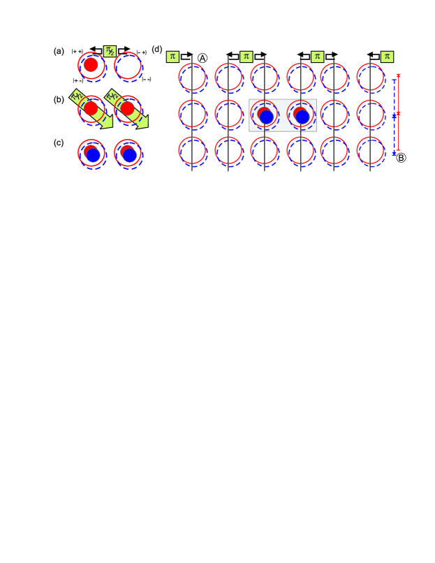
Figure 6: (Color online) Implementation of the coin and the coin operator $C_{\text{2D}}=\textrm{{H}}_{\text{SD}}\otimes\textrm{{H}}_{\text{HF}}$ for the two-dimensional walk: (a) The four levels are formed as a tensor product of a delocalized qubit (left and right traps) and a hyperfine qubit (dark and grey filled circles symbolize the $|+\rangle$ and $|-\rangle$ hyperfine states, full and dashed lines denote the respective trapping potentials). The initial state is $|++\rangle$. (a)$\rightarrow$(b) For $\textrm{{H}}_{\text{SD}}$ the traps are approached (for both hyperfine states). (b)$\rightarrow$(c) For $\textrm{{H}}_{\text{HF}}$ a $\pi/2$ pulse between the two hyperfine levels is applied to all traps simultaneously. (d) The implementation of the two-dimensional walking operator $O_{\text{2D}}$ as a combination of tunneling and spin dependent transport: (A) traps in horizontally adjacent traps are approached to give a $\pi$-pulse as in the one-dimensional walk; (B) the lattice is displaced in opposite vertical directions for the two hyperfine states.

There is no unique extension of the Hadamard operator H to $\mathcal{H}_{C}$ from Eq. (7), because different classes of unbiased coin operators for two-dimensional walks exist coinsandstates . The most obvious and simple generalization is to take a Hadamard coin for both directions. This can be realized by first approaching the traps to perform a $\pi/2$ pulse for the delocalized qubit as above, and then putting the atom in a superposition of the two hyperfine levels by a $\pi/2$ two-photon twophoton or microwave QWOptLat pulse, which realizes $C_{\text{2D}}=\textrm{{H}}_{\text{HF}}\otimes\textrm{{H}}_{\text{SC}}$ (c.f. Fig. 6 (a-c) for the case of $|++\rangle$ as initial state). For the coin-dependent displacement assume that at each vertex of the two-dimensional grid each two traps forming a coin are aligned horizontally. Then in horizontal direction first the walking operator $O_{\text{1D}}$ can be applied, i.e., within each row traps of neighboring qubits are approached as described above to give a $\pi$ pulse, followed by translating the lattice potential in opposite vertical directions for each spin state, as proposed in QWOptLat (see Fig. 6 (d)). In total, the action of the walking operator $O_{\text{2D}}$ in $\mathcal{H}_{W}\otimes\mathcal{H}_{C}$ is given by

$$O_{\text{2D}}|(k,l),\pm\pm\rangle=|(k\pm 1,l\pm 1),\mp\pm\rangle.$$ (8)

Fig. 7 shows a probability distributions arising from alternatingly applying $\mathbb{I}\otimes C_{\text{2D}}$ and $O_{\text{2D}}$ to the initial state $|\psi_{\text{init}}\rangle=|(0,0),++\rangle$. From its construction it is easy to see that the coin operator $C_{\text{2D}}$ does not mix the horizontal and vertical direction. For this reason one recovers the one-dimensional quantum walk when projecting the distributions along the $x$ or $y$ directions (due to the choice of the initial conditions the distribution is not symmetric in this case). $C_{\text{2D}}$ is thus a separable Hadamard walk according to the classification of QWmoreDim .

(I)

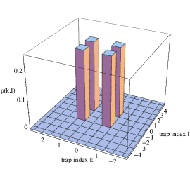
(II)

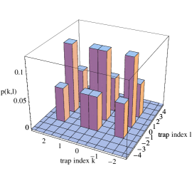
(III)

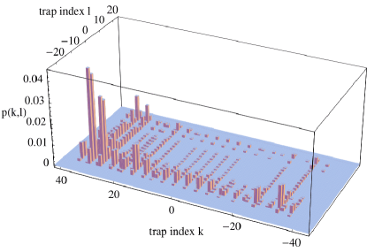
Figure 7: (Color online) Probability distributions for the two-dimensional quantum walk obtained from alternatingly applying $C_{\text{2D}}$ and $O_{\text{2D}}$ to the initial state $|\psi_{\text{init}}\rangle=|(0,0),++\rangle$ after (I) $t=1$, (II) $t=2$, and (III) $t=25$ steps. The coordinates on $k$ and $l$ axes label the traps, thus in k direction each two traps form one site; note that the total population of each trap is shown (sum of probabilities for both hyperfine states).

IV.0.2 Entangled walks

More sophisticated coin operators are also possible, and we will show how to implement one which entangles the two directions. Assuming to be able to change the trapping potentials for both hyperfine states independently, we can apply a $\pi/2$ pulse (Hadamard operation) on delocalized qubit for the $|+\rangle$ hyperfine state and a $\pi/2$ pulse followed by a $\pi$ pulse ($X_{\textrm{{NOT}}}$ operation) on the delocalized qubit for the $|-\rangle$ hyperfine state. Subsequently a $\pi/2$ pulse is applied tothe hyperfine qubit as before. Then, defining the $X_{\textrm{{NOT}}}$ operation as,

$$X_{\textrm{{NOT}}} = \left(\begin{matrix}0&1\\ 1&0\end{matrix}\right),$$ (9)

the full coin operator reads

$$C_{\text{2D}}^{\text{Ent}} = \left(\mathbb{I}\otimes\textrm{{H}}^{\text{HF}}\right)\cdot\left(\textrm{{H}}^{\text{SD}}\otimes|+\rangle\!\langle+|+\right.$$ (10a)

$$\left.+X_{\textrm{{NOT}}}^{\text{SD}}\textrm{{H}}^{\text{SD}}\otimes|-\rangle\!\langle-|\right)$$

$$= \frac{1}{2}\left(\begin{matrix}1&1&1&-1\\ 1&-1&1&1\\ 1&1&-1&1\\ 1&-1&-1&-1\end{matrix}\right).$$ (10b)

(Similary, given local addressability, different laser pulses could be applied to the two traps forming the spatially delocalized qubit). The operator $C_{\text{2D}}^{\text{Ent}}$ is non-separable QWmoreDim ; coinsandstates . The result for the initial state $|\psi_{\text{init}}\rangle=|(0,0),++\rangle$ is shown in Fig. 8. Similar sequences of operations can be used to generate different coin operators. It has been noted in coinsandstates that even for a fixed entangling coin operator very different probability distributions can be obtained through varying the initial state. At least for a system of optical microtraps it should be possible to engineer the initial state carefully enough, because due to the large separation of traps, single sites can easily be addressed. In this way these systems can be an interesting testbed to explore the rich structure of probability distributions of two-dimensional quantum walks.

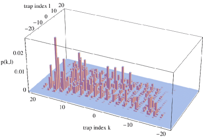
Figure 8: (Color online) Probability distribution of the two-dimensional quantum walk with the coin operator $C_{\text{2D}}^{\text{Ent}}$ after $t=25$ steps. The initial state is $|\psi_{\text{init}}\rangle=|(0,0),++\rangle$.

Recently Ambainis et al. proposed a quantum search algorithm to locate a single marked site among $N$ locations arranged on a square $\sqrt{N}\times\sqrt{N}$ grid using a total number of $O(\sqrt{N}\log^{2}N)$ steps, thus outperforming Grovers algorithm in this case coinsfaster , where the time to move between locations is taken into account. The algorithm is based on a quantum walk on a two dimensional lattice with (i) periodic boundary conditions, (ii) a special coin as well as a special displacement operator, and (iii) a certain initial state. We will show how to realize the basic ingredients (ii) and (iii) within our proposal. The realization of periodic boundary conditions however is not straightforward for the setup proposed here, but might be achievable with more advanced setups. Fixed boundaries can be imposed for optical microtraps by only illuminating a rectangular subset of lenses and applying an additional $\pi/2$ pulse on the hyperfine qubits on the borders of the lattice. Numerically we observe that the effect of a large amplitude at the marked site is still present for such boundary conditions, though the effect on the performance of the algorithm needs further investigation.

The required displacement operator is the two-dimensional version of the flip-flop walking operator which we already saw in the one-dimensional realization. It reads

$$O_{\text{FF}}|(k,l),\pm\pm\rangle=|(k\pm 1,l\pm 1),\mp\mp\rangle,$$ (11)

i.e., the walk changes direction after each step, and obviously here it can be realized by a $\pi$-pulse on the hyperfine qubit after applying $O_{\text{2D}}$. The coin operator has to be chosen as

$$C_{0}=\frac{1}{2}\left(\begin{matrix}-1&1&1&1\\ 1&-1&1&1\\ 1&1&-1&1\\ 1&1&1&-1\end{matrix}\right),$$ (12)

except for the marked vertex, for which

$$C_{1}=\left(\begin{matrix}-1&0&0&0\\ 0&-1&0&0\\ 0&0&-1&0\\ 0&0&0&-1\end{matrix}\right)$$ (13)

is applied. For an implementation of the search algorithm, these operators have to be constructed as a suitable combination of operations on the hyperfine and the delocalized qubit. We will require the manipulation of the delocalized qubit to act identically on all sites, but in order to engineer a special coin operator for the marked vertex, for the manipulation of the hyperfine state we will assume to be able to address single sites. We define a single qubit phase gate

$$X_{\textrm{{PHASE}}}=\left(\begin{matrix}1&0\\ 0&-1\end{matrix}\right),$$ (14)

and

$$X^{\prime}_{\textrm{{NOT}}} = |+\rangle\!\langle+|\otimes X_{\textrm{{NOT}}}^{\text{HF}}+|-\rangle\!\langle-|\otimes\mathbb{I},$$ (15)

as an operator which produces a $\pi$ pulse only on one trap of each coin. Then

$$-C_{0} = X^{\prime}_{\textrm{{NOT}}}\cdot\left(\textrm{{H}}^{\text{SD}}\otimes X_{\textrm{{PHASE}}}^{\text{H}F}\right)\cdot X^{\prime}_{\textrm{{NOT}}}\cdot$$ (16)

$$\left(\textrm{{H}}^{\text{SD}}\otimes X_{\textrm{{PHASE}}}^{\text{H}F}\right)\cdot X^{\prime}_{\textrm{{NOT}}}$$

produces, except for an overall phase, the correct coin operator. The operator for the marked vertex is obtained by merely replacing the $X^{\prime}_{\textrm{{NOT}}}$ operator by $\mathbb{I}$:

$$-C_{1} = \left(\textrm{{H}}^{\text{SD}}\otimes X_{\textrm{{PHASE}}}^{\text{H}F}\right)\cdot\left(\textrm{{H}}^{\text{SD}}\otimes X_{\textrm{{PHASE}}}^{\text{H}F}\right).$$ (17)

Thus, given the possibility to locally manipulate the hyperfine qubit and except for a global phase, the quantum search coin operators can be constructed. Finally, the initial state has to be chosen as an eigenstate of $O_{FF}\cdot(\mathbb{I}\otimes C_{0})$. For fixed boundaries, such an eigenstate is given by

$$|\Phi_{0}\rangle=\frac{1}{2\sqrt{N}}\sum_{k=1}^{\sqrt{N}}\sum_{l=1}^{\sqrt{N}}\sum_{\alpha\in\{+,-\}}\sum_{\beta\in\{+,-\}}|(k,l),\alpha\>\beta\rangle,$$

which can be generated by a sequence of shift operations firstly via tunneling and secondly via displacements of the state-dependent lattices coinsfaster .

V Summary

We have discussed the implementation of quantum walks with a neutral atom trapped in the ground state of optical potentials by using the concept of spatially delocalized qubits, i.e., a coin defined through the presence of the atom in one out of two trapping potentials. We have shown that in this case a quantum walk on a line can be performed in a simple way only through a variation of the trapping potentials, without the need for additional lasers to address internal states of the atom. Our simulations were performed with realistic parameters for present optical microtrap systems, but the concept is as well applicable to optical lattices or to magnetic microtraps. We have studied the influences of various experimental imperfections on the probability distribution and have found a strong change if the atom is initially not in the ground state of the trap. This change, leading to a strong dependence of the quantum walk on temperature, can be attributed to non-adiabatic excitations to other vibrational states during the movement of the traps. We have also studied the influence of shaking and found a transition from quantum to classical probability distributions, taking place for shaking amplitudes on the order of $1$% of the tunneling distance. As an intermediate step, this transition exhibits a very flat distribution. An estimate of other decoherence effects such as scattering of photons from the trapping lasers suggests that quantum walks should be observable in the experiment and the effects of temperature and shaking should be accessible to experimental investigation. In this way, implementing the quantum walk with spatially delocalized coins could give information on the extend to which the ground state population and the movement of the traps can be controlled.

Finally, we have combined the concept of the spatially delocalized qubit with a hyperfine qubit and state dependent potentials to obtain a scheme to implement a quantum walk on a two-dimensional regular lattice. Within this scheme, which again is close to what is realizable with state-of-the-art technology in optical microtraps as well as in optical lattices, different coin operators are possible, such that in this setup the variety of different distributions in two-dimensional quantum walks can be explored. Especially we have shown how to construct separable and entangling coin operators, as well as the operators necessary to implement a spatial search algorithm on a two-dimensional grid. It is worth stressing that the scheme proposed by us can be used to construct the generalized coined quantum walk, in which the walker acquires at each step a phase phase .

VI Acknowledgments

This work has been supported by the European Community through the HPC-Europe program, by the European Commission through IST projects EQUIP and ACQP, by the DFG (Schwerpunktprogramm ’Quanteninformationsverarbeitung’ and SFB 407) and from the MCyT (Spanish Government) and the DGR (Catalan Government) under contract BFM2002-04369-C04-02 and 2001SGR00187, respectively. We thank D. Bruß, R. Corbalán, R. Dumke, W. Ertmer, A. Lengwenus, T. Müther, U. Poulsen, A. Sanpera, and M. Volk for discussions.

References

- (1) R. Motwani and P. Raghavan, Randomized algorithms, Cambridge Univ. Press (1995)
- (2) A. Childs, E. Farhi, and S. Gutmann, Quant. Inf. Proc. 1, 35 (2002).
- (3) J. Kempe, Cont. Phys. 44 , 307 (2003).
- (4) D. Aharonov, A. Ambainis, J. Kempe, and U. Vazirani, Proc. ACM Symp. Th. of Comp. (STOC’01), 50 (2001).
- (5) A. Nayak and A. Vishwanath, quant-ph/0010117 (2000);
- (6) T.D. Mackay, S.D. Bartlett, L.T. Stephenson, and B.C. Sanders, J. Phys. A 35, 2745 (2002).
- (7) J. Kempe, in Proc. of 7th Intern. Workshop on Randomization and Approximation Techniques in Comp. Sc., p. 354 (2003).
- (8) A.M. Childs, R. Cleve, E. Deotto, E. Farhi, S. Gutmann, and D.A. Spielman, Proc. 35th ACM Symposium on Theory of Computing, 59 (2003).
- (9) N. Shenvi, J. Kempe, and K.B. Whaley, Phys. Rev. A 67, 052307 (2003).
- (10) A.M. Childs and J. Goldstone, Phys. Rev. A 70, 022314 (2004).
- (11) A. Ambainis, J. Kempe, and A. Rivosh, quant-ph/0402107 (2004).
- (12) B.C. Travaglione and G.J. Milburn, Phys. Rev. A 65, 032310 (2002).
- (13) W. Dür, R. Raussendorf, V.M. Kendon, and H.J. Briegel, Phys. Rev. A 66, 052319 (2002).
- (14) Z. Zhao, J. Du, H. Li, T. Yang, Z. Chen, and J. Pan, quant-ph/0212149 (2002).
- (15) P.L. Knight, E. Roldan, and J.E. Sipe, Phys. Rev. A 68, 020301(R) (2003).
- (16) J. Mompart, K. Eckert, W. Ertmer, G. Birkl, and M. Lewenstein, Phys. Rev. Lett. 90, 147901 (2003).
- (17) for an overview see: P. S. Jessen and I. H. Deutsch, Adv. At. Mol. Opt. Phys. 36, 91 (1996); G. Grynberg and C. Robilliard, Phys. Rep. 355, 355 (2001).
- (18) for an overview see: R. Folman, P. Krüger, J. Schmiedmayer, J. Denschlag, and C. Henkel, Adv. At. Mol. Opt. Phys. 48, 263 (2002).
- (19) R. Dumke, M. Volk, T. Muether, F.B.J. Buchkremer, G. Birkl, and W. Ertmer, Phys. Rev. Lett. 89, 097903 (2002).
- (20) H. Jeong, M. Paternostro, and M.S. Kim, Phys. Rev. A 69, 012310 (2004).
- (21) E. Roldan and J.C. Soriano, quant-ph/0503069 (2005).
- (22) D. Jaksch, H.J. Briegel, J.I. Cirac, C.W. Gardiner, and P. Zoller, Phys. Rev. Lett 82 1975 (1999).
- (23) Y. Omar, N. Paunkovic, L. Sheridan, and S. Bose, quant-ph/0411065 (2004).
- (24) D. Meyer, J. Stat. Phys. 85, 551 (1996).
- (25) B. Tregenna, W. Flanagan, R. Maile, and V. Kendon, New J. Phys. 5, (2003).
- (26) S. Bergamini, D. Darqui’e, M. Jones, L. Jacubowiez, A. Browaeys, and P. Grangier, J. Opt. Soc. Am. B 21, 1889 (2004).
- (27) E. Charron, E. Tiesinga, F. Mies, and C. Williams, Phys. Rev. Lett. 88, 077901 (2002).
- (28) R. Scheunemann, F. S. Cataliotti, T. W. Hänsch, and M. Weitz, Phys. Rev. A 62, 051801(R) (2000).
- (29) W. Hänsel, J. Reichel, P. Hommelhoff, and T. W. Hänsch, Phys. Rev. A 64, 063607 (2001).
- (30) S. E. Hamann, D. L. Haycock, G. Klose, P. H. Pax, I. H. Deutsch, and P. S. Jessen , Phys. Rev. Lett. 80, 4149 (1998).
- (31) V. Kendon and B. Tregenna, Lecture Notes Phys. 633, 253 (2003); V. Kendon and B. Tregenna, Phys. Rev. A 67, 042315 (2003).
- (32) G. Birkl, F.B.J. Buchkremer, R. Dumke, and W. Ertmer, Optics Comm. 191, 67 (2001).
- (33) O. Mandel, M. Greiner, A. Widera, T. Rom, T. W. Hänsch, and I. Bloch, Phys. Rev. Lett. 91, 010407 (2003); G. K. Brennen, C. M. Caves, P. S. Jessen, and I. H. Deutsch, Phys. Rev. Lett. 82, 1060 (1999); D. Jaksch, H.-J. Briegel, J. I. Cirac, C. W. Gardiner, and P. Zoller Phys. Rev. Lett. 82, 1975 (1999).
- (34) see E. Arimondo, in Progress in Optics, edited by E. Wolf (Elsevier Science, Amsterdam, 1996), Vol. 35, p. 257; and references therein
- (35) A. Wójcik, T. Łuczak, P. Kurzyński, A. Grudka, and M. Bednarska, Phys. Rev. Lett 93, 180601 (2004).