Entanglement in $SO(3)$-invariant bipartite quantum systems

Abstract

The structure of the state spaces of bipartite $N\otimes N$ quantum systems which are invariant under product representations of the group $SO(3)$ of three-dimensional proper rotations is analyzed. The subsystems represent particles of arbitrary spin $j$ which transform according to an irreducible representation of the rotation group. A positive map $\vartheta$ is introduced which describes the time reversal symmetry of the local states and which is unitarily equivalent to the transposition of matrices. It is shown that the partial time reversal transformation $\vartheta_{2}=I\otimes\vartheta$ acting on the composite system can be expressed in terms of the invariant $6$-$j$ symbols introduced by Wigner into the quantum theory of angular momentum. This fact enables a complete geometrical construction of the manifold of states with positive partial transposition and of the sets of separable and entangled states of $4\otimes 4$ systems. The separable states are shown to form a three-dimensional prism and a three-dimensional manifold of bound entangled states is identified. A positive maps is obtained which yields, together with the time reversal, a necessary and sufficient condition for the separability of states of $4\otimes 4$ systems. The relations to the reduction criterion and to the recently proposed cross norm criterion for separability are discussed.

I Introduction

It is one of the basic postulates of quantum mechanics that the Hilbert space of states of a composite system is given by the tensor product of the Hilbert spaces pertaining to its subsystems. If a system is composed of two $N$-state systems with Hilbert space ${\mathcal{H}}={\mathbb{C}}^{N}$, the mixed states of the total system are represented by density matrices which act on the tensor product ${\mathbb{C}}^{N}\otimes{\mathbb{C}}^{N}$. A state of such an $N\otimes N$ system is said to be separable or classically correlated if it can be generated by mixing with certain probabilities an ensemble of states which describe statistically independent subsystems WERNER . States which cannot be represented in this way are called inseparable or entangled. The characterization, classification and quantification of mixed-state entanglement and the development of explicit necessary and sufficient separability criteria turn out to be an extremely hard problem ECKERT . The solution of this problem could have far-reaching consequences for fundamental questions of quantum mechanics and computational complexity theory NIELSEN00 and for applications in the theory of quantum information ALBER ; NIELSEN .

A great simplification of the entanglement problem is obtained though the introduction of symmetries WERNER ; VOLLBRECHT ; BRACKEN . By the requirement of invariance under certain groups of symmetry transformations one restricts the set of all states to a low-dimensional manifold of invariant states and one may hope to get a tractable problem which is solvable with the help of group theoretical and algebraic methods. A prominent example is given by the one-parameter family of the Werner states WERNER which results from the requirement of invariance under all product transformations of the form $U\otimes U$, where $U$ varies over the full group of unitary $N\times N$ matrices. A further related example is the one-parameter family of isotropic states HORODECKI99 ; RAINS which are invariant under all product unitaries $U\otimes U^{*}$, where $U^{*}$ denotes the complex conjugation of $U$. Imposing the invariance under all transformations of the form $O\otimes O$, where $O$ belongs to the group of orthogonal $N\times N$ matrices, one obtains the two-dimensional manifold of orthogonally invariant states VOLLBRECHT . It is clear that the larger the symmetry group the smaller is the remaining space of invariant states and the easier should be the analysis of its structure. In fact, the problem of the explicit determination of the separable states under symmetry requirements can be solved completely for the examples given above.

A physically natural symmetry group is the group $SO(3)$ of proper rotations in three dimensions. The underlying assumption is that the states of the subsystems transform according to an $N=(2j+1)$-dimensional irreducible representation of the rotation group which corresponds to a fixed angular momentum $j$. The subsystems thus behave under rotations as particles with a certain spin $j$. The rotation group then operates through a reducible product representation on the states of the composite system. Any $SO(3)$-invariant state can be decomposed into a sum of projections onto the irreducible subspaces belonging to the various eigenvalues $J=0,1,\ldots,2j$ of the total angular momentum operator. This shows that the rotationally invariant states form an $(N-1)$-dimensional manifold. The requirement of $SO(3)$ invariance reduces the full $(N^{4}-1)$-dimensional space of all mixed states of an $N\otimes N$ system to an $(N-1)$-dimensional space of invariant states.

The invariance under $SO(3)$ transformations represents in general a much smaller symmetry than those of the examples given above. For example, the manifolds of the Werner states and of the isotropic states can be embedded into the set of rotationally invariant states. These examples are thus special cases of the $SO(3)$ symmetry.

The problem of mixed-state entanglement in $SO(3)$-invariant bipartite systems will be analyzed in this paper. We find that the state spaces exhibit an interesting convex structure and several important phenomena as the emergence of non-decomposable positive maps WORONOWICZ and bound entanglement HORODECKI98 . The physical significance of the $SO(3)$ symmetry derives from the fact that any rotationally invariant state can be produced from the maximally entangled angular momentum singlet state $J=0$ through the application of an isotropic dynamical map which operates locally on the subsystems. The set of $SO(3)$-invariant states is thus identical to the set of states which results from interactions of the singlet state with noisy isotropic environments.

A powerful tool in studies of entanglement is the operation of taking the partial transposition of states. The requirement of positive partial transposition (PPT) represents a strong necessary condition for the separability of states, known as the Peres criterion PERES . A conceptually simple but crucial point of the present investigation consists in the replacement of the transposition by another unitarily equivalent operation which is identical to the time reversal transformation of particles with spin $j$. It is known that the anti-unitary operation of the time reversal commutes with the representations of the rotation group. This fact allows one to characterize the partial transposition by means of invariant quantities which are directly related to Wigner’s $6$-$j$ symbols WIGNER .

The $6$-$j$ symbols arise in the transformation between different coupling schemes for the addition of angular momenta EDMONDS . They can be expressed as invariant sums over products of vector-coupling (Clebsch-Gordan) coefficients. Thus we find a close connection between the partial transposition, the time reversal symmetry and certain group-theoretical invariants built out of the vector-coupling coefficients. It will be demonstrated here that this connection to group-theoretical concepts leads to important implications on the entanglement structure of the state space.

The content of the paper can be summarized as follows. In Sec. II we briefly recall some facts from the representation theory of the rotation group and introduce an appropriate parametrization of the set of rotationally invariant states. The partial transposition and the corresponding transformation of the partial time reversal are discussed in Sec. III. It is shown that this transformation preserves the rotational invariance of states and its relation to the Wigner $6$-$j$ symbols is derived.

These results are used in Secs. IV and V to develop a geometric representation of the sets of the PPT states and of the separable states in the cases $N=2$, $3$ and $4$. Most importantly, in the case $N=4$ we find that the set of separable states is isomorphic to a three-dimensional prism, i. e., to a polyhedron which is bounded by three squares and two triangles. We further identify a three-dimensional manifold of bound entangled states with positive partial transposition.

Finally, Sec. VI contains a discussion of the results and a number of conclusions which can be drawn from the present investigation. In particular, we construct a positive map which yields, together with the time reversal, a necessary and sufficient condition for separability in the case of $4\otimes 4$ systems. Moreover, we discuss the relations to two further criteria of separability, namely the reduction criterion and the cross norm criterion.

II The set of $SO(3)$-invariant states

II.1 Representations of the rotation group

We consider a bipartite quantum system whose local parts are $N$-state systems with corresponding state space ${\mathcal{H}}={\mathbb{C}}^{N}$. The Hilbert space of the composite system is given by the tensor product space ${\mathcal{H}}\otimes{\mathcal{H}}$. The local state spaces are regarded as angular momentum manifolds corresponding to a certain eigenvalue of the square of the angular momentum operator $\hat{\bm{j}}$. Thus, the state space ${\mathcal{H}}$ is spanned by a fixed orthonormal basis of $N=(2j+1)$ angular momentum eigenvectors $|jm\rangle$, where $m=-j,-j+1,\ldots,+j$. As usual we have the eigenvector relations $\hat{\bm{j}}^{2}|jm\rangle=j(j+1)|jm\rangle$ and $\hat{j}_{3}|jm\rangle=m|jm\rangle$. Note that $j$ can take on integer or half-integer values, $j=\frac{1}{2},1,\frac{3}{2},\ldots$, such that $N=2,3,4,\ldots$

The group of proper rotations in three dimension is denoted by $SO(3)$. This is the group of orthogonal $3\times 3$ matrices with determinant $1$. An irreducible representation of this group on the state space ${\mathcal{H}}$ is obtained in the standard way: Given a rotation $R\in SO(3)$ the corresponding transformation of state vectors is provided by the unitary matrix

$$D(R)=D(n_{1},n_{2},n_{3})=\exp\left(-i\bm{n}\cdot\hat{\bm{j}}\right).$$ (1)

The rotation $R$ is characterized here by the vector ${\bm{n}}=(n_{1},n_{2},n_{3})$, i. e., $R$ is the rotation about the axis given by $\bm{n}$ by the angle $|\bm{n}|$ (in a right-handed sense). It should be mentioned that Eq. (1) generally yields a two-valued representation of the rotation group: For half-integer $j$ one obtains two unitary matrices which represent a given rotation $R$ and which differ in sign.

II.2 Rotational invariance of bipartite systems

The representation (1) leads to a representation of the rotation group on the tensor product space ${\mathcal{H}}\otimes{\mathcal{H}}$ of the bipartite system. If $\rho$ is an operator acting on the tensor product space, a rotation $R$ carried out on both parts of the composite system leads to the transformed operator $\rho^{\prime}=[D(R)\otimes D(R)]\rho[D(R)\otimes D(R)]^{\dagger}$. An operator $\rho$ is said to be rotationally invariant or $SO(3)$-invariant if it is invariant under all such transformation, that is, if the relation

$$[D(R)\otimes D(R)]\rho[D(R)\otimes D(R)]^{\dagger}=\rho$$ (2)

holds for all $R\in SO(3)$.

A state of the bipartite system is given by a density matrix $\rho$ satisfying $\rho\geq 0$ and ${\mathrm{tr}}\rho=1$. The set of all states $\rho$ which fulfill the invariance requirement (2) will be denoted by $S$. It is clear that $S$ is a convex subset of the set of all states of the bipartite system.

The angular momentum operator of the composite system is given by $\hat{\bm{J}}=\hat{\bm{j}}\otimes I+I\otimes\hat{\bm{j}}$, where $I$ denotes the unit matrix. The components of $\hat{\bm{J}}$ are the generators of the product representation and the requirement of rotational invariance is equivalent to the statement that $\rho$ commutes with all components of $\hat{\bm{J}}$.

The product representation $D(R)\otimes D(R)$ is obviously reducible. Its decomposition into a sum of irreducible representations is a standard subject of quantum mechanics. One introduces an orthonormal basis in ${\mathcal{H}}\otimes{\mathcal{H}}$ which consists of the common eigenvectors $|JM\rangle$ of $\hat{\bm{J}}^{2}$ and $\hat{J}_{3}$ corresponding to the eigenvalues $J(J+1)$ and $M$, respectively, where $J=0,1,\ldots,2j$ and $M=-J,-J+1,\ldots,+J$. The $(2J+1)$-dimensional space which is spanned by the basis vectors $|JM\rangle$ with a fixed $J$ is an invariant and irreducible subspace of the tensor product representation.

The set $S$ of rotationally invariant operators can now easily be characterized. To this end, we introduce projection operators

$$P_{J}=\sum_{M=-J}^{+J}|JM\rangle\langle JM|$$ (3)

which project onto the subspaces belonging to a fixed $J$. From the irreducibility of the representation within these subspaces one concludes with the help of Schur’s lemma that any rotationally invariant operator $\rho$ can be written as a linear combination of the projections:

$$\rho=\frac{1}{N}\sum_{J=0}^{2j}\frac{\alpha_{J}}{\sqrt{2J+1}}P_{J}.$$ (4)

Here, the $\alpha_{J}$ are c-numbers and we have introduced normalization factors $(N\sqrt{2J+1})^{-1}$. It will be seen in Sec. III.4 that this choice of normalization factors leads to highly symmetric transformation properties of the parameter space. For $\rho$ to be Hermitian the $\alpha_{J}$ must of course be real. Equation (4) then corresponds to the spectral decomposition of $\rho$. If $\rho$ is a density matrix the $\alpha_{J}$ are real and positive, $\alpha_{J}\geq 0$. On using ${\mathrm{tr}}P_{J}=2J+1$, the normalization condition takes the form

$${\mathrm{tr}}\rho=\sum_{J=0}^{2j}\frac{\sqrt{2J+1}}{N}\alpha_{J}=1.$$ (5)

For example, setting $\alpha_{0}=N$ and $\alpha_{J}=0$ for $J=1,2,\ldots,2j$ we get $\rho=P_{0}=|00\rangle\langle 00|$, i. e., the projection onto the angular momentum singlet state

$$|00\rangle=\frac{1}{\sqrt{N}}\sum_{m=-j}^{+j}(-1)^{j-m}|j,m\rangle\otimes|j,-m\rangle.$$ (6)

This state is the only pure state in $S$ and it is maximally entangled (the quantity $\frac{\alpha_{0}}{N}$ is the singlet fraction). Using the completeness of the projections $P_{J}$ one concludes that the state corresponding to $\alpha_{J}=\sqrt{2J+1}/N$, $J=0,1,\ldots,2j$, is the separable state $\rho=\frac{1}{N^{2}}I\otimes I$ of maximal entropy.

It follows from the irreducibility of the representation $D(R)$ that for any $SO(3)$-invariant state $\rho$ the reduced density matrices $\rho^{(1)}={\mathrm{tr}}_{2}\rho$ and $\rho^{(2)}={\mathrm{tr}}_{1}\rho$ of the subsystems, given by the partial traces ${\mathrm{tr}}_{2}$ and ${\mathrm{tr}}_{1}$, are proportional to the identity $I$. The reduced density matrices obtained from a rotationally invariant state thus describe states of maximal disorder.

Summarizing, by means of Eq. (4) any rotationally invariant Hermitian operator is uniquely characterized by $N$ real parameters $\alpha_{J}$. We can therefore identify the set of all such operators with the set of points

$${\bm{\alpha}}=\left(\begin{array}[]{c}\alpha_{0}\\ \alpha_{1}\\ .\\ .\\ \alpha_{2j}\end{array}\right)\in{\mathbb{R}}^{N}$$ (7)

in an $N$-dimensional parameter space ${\mathbb{R}}^{N}$. The set of points $\bm{\alpha}$ in this space satisfying $\alpha_{J}\geq 0$ and the normalization condition (5) then describes the set $S$ of rotationally invariant density matrices. In geometrical terms $S$ represents an $(N-1)$-dimensional simplex. For instance, $S$ is a line for $N=2$, a triangle for $N=3$, and a tetrahedron for $N=4$. These examples will be discussed in Secs. IV.2 and V.3.

III Positive maps and rotational invariance

III.1 Partial transposition

Given an operator $B$ on ${\mathcal{H}}$ the transposed operator $TB=B^{T}$ is defined in terms of the local basis states $|jm\rangle$ by means of $\langle jm|B^{T}|jm^{\prime}\rangle\equiv\langle jm^{\prime}|B|jm\rangle$. Correspondingly, the partial transposition $T_{2}=I\otimes T$ on the tensor product space is defined through

$$T_{2}(A\otimes B)=A\otimes TB=A\otimes B^{T}.$$ (8)

The operation of taking the partial transpose plays an important role in entanglement and quantum information theory. One reason for this fact is that $T$ is a distinguished example of a map which is positive but not completely positive STINESPRING ; CHOI1 ; CHOI2 ; WORONOWICZ ; KRAUS1 ; KRAUS2 . This means that $T$ takes positive operators on ${\mathcal{H}}$ to positive operators on ${\mathcal{H}}$, while $T_{2}\rho$ need not be positive for a positive operator $\rho$ on the tensor product space ${\mathcal{H}}\otimes{\mathcal{H}}$.

Important information on the entanglement structure of states is obtained by considering the action of positive but not completely positive maps. An example is given by the Peres PPT criterion according to which positivity under the partial transposition $T_{2}$ is a necessary condition for separability PERES . An important general characterization has been developed by the Horodecki’s HORODECKI96a : A necessary and sufficient condition for a state $\rho$ to be separable is that the operator $(I\otimes\Phi)\rho$ is positive for any positive map $\Phi$. This condition does however not lead to a simple operational criterion for separability since we have no general structural characterization of positive maps, as it exists for completely positive maps in the form of the Kraus-Stinespring representation STINESPRING ; KRAUS1 ; KRAUS2 .

III.2 $\vartheta_{2}$-transformation

If $\rho$ is a rotationally invariant operator the partially transposed operator $T_{2}\rho$ is generally not invariant under rotations. It can be shown that, instead, $T_{2}\rho$ is invariant under transformations of the form $D(R)\otimes D(R)^{*}$, where $D(R)^{*}$ is the matrix obtained from $D(R)$ by complex conjugation of its elements, that is $D(R)^{*}=D(R)^{\dagger T}$. Throughout this paper $T$ denotes the transposition, $\dagger$ the adjoint and $\ast$ the element-wise complex conjugation of a matrix.

In the present investigation we shall utilize a map which is unitarily equivalent to the partial transposition, but which does map rotationally invariant operators to rotationally invariant operators. This map will be denoted by $\vartheta_{2}$. By analogy to Eq. (8), $\vartheta_{2}$ is taken to be of the form

$$\vartheta_{2}(A\otimes B)=A\otimes\vartheta B=A\otimes VB^{T}V^{\dagger}$$ (9)

with some fixed unitary matrix $V$. Hence, $\vartheta_{2}=I\otimes\vartheta$ is the partial transposition $T_{2}$ followed by a local unitary transformation acting on the second part of the bipartite system, that is, we have $\vartheta_{2}\rho=(I\otimes V)T_{2}\rho(I\otimes V)^{\dagger}$. Since the maps $\vartheta_{2}$ and $T_{2}$ are unitarily equivalent a state $\rho$ is obviously positive under $\vartheta_{2}$ if and only if it is positive under $T_{2}$.

The unitary matrix $V$ will be determined from the condition that $\vartheta_{2}$ preserves the rotational invariance of operators, i. e., if $\rho$ is any invariant operator satisfying Eq. (2) we demand that the transformed operator $\vartheta_{2}\rho$ is again invariant:

$$[D(R)\otimes D(R)]\vartheta_{2}\rho[D(R)\otimes D(R)]^{\dagger}=\vartheta_{2}\rho.$$ (10)

This requirement is obviously satisfied if the map $\vartheta$ commutes with all rotations, that is, if the relation

$$\vartheta[D(R)BD(R)^{\dagger}]=D(R)(\vartheta B)D(R)^{\dagger}$$ (11)

holds true for all operators $B$ on ${\mathcal{H}}$ and all $R\in SO(3)$. By use of the definition of $\vartheta$ given by Eq. (9) one can write Eq. (11) as

$$VD(R)^{*}B^{T}[VD(R)^{*}]^{\dagger}=D(R)VB^{T}[D(R)V]^{\dagger}.$$ (12)

This equation is fulfilled if $VD(R)^{*}=D(R)V$. Thus we see that the rotational invariance of $\vartheta_{2}\rho$ follows from the rotational invariance of $\rho$ provided we can find a fixed unitary matrix $V$ such that

$$VD(R)^{*}V^{\dagger}=D(R)$$ (13)

for all $R\in SO(3)$.

To obtain a unitary matrix $V$ satisfying Eq. (13) we employ specific properties of the representations of the rotation group. As in Eq. (1), let $D(R)$ be the representation of the rotation $R$ about an axis $\bm{n}=(n_{1},n_{2},n_{3})$ by an angle $|\bm{n}|$. The complex conjugation of the elements of $D(R)$ then yields the matrix

$$D(R)^{*} = \exp\left(+i\bm{n}\cdot\hat{\bm{j}}^{T}\right)$$ (14)

$$= \exp\left(-i[-n_{1}\hat{j}_{1}+n_{2}\hat{j}_{2}-n_{3}\hat{j}_{3}]\right)$$

$$= \exp\left(-i\bm{n}^{\prime}\cdot\hat{\bm{j}}\right).$$

Here we use the fact that in the local basis $|jm\rangle$ the transposed components of the angular momentum operator are given by $\hat{j}_{1}^{T}=\hat{j}_{1}$, $\hat{j}_{2}^{T}=-\hat{j}_{2}$ and $\hat{j}_{3}^{T}=\hat{j}_{3}$. Thus, $D(R)^{*}$ represents the rotation about the axis ${\bm{n}}^{\prime}=(-n_{1},n_{2},-n_{3})$ which is obtained from ${\bm{n}}$ through a rotation by $\pi$ about the $x_{2}$-axis. To transform from $D(R)^{\ast}$ to $D(R)$ we therefore define $V$ to be the matrix representing a $\pi$-rotation about the $x_{2}$-axis. Using the notation introduced in Eq. (1) we write

$$V\equiv D(0,\pi,0).$$ (15)

Explicitly the matrix elements of $V$ are given by

$$\langle jm^{\prime}|V|jm\rangle=(-1)^{j-m}\delta_{m^{\prime},-m}.$$ (16)

Hence, $V$ is real and we have $V^{T}=V^{\dagger}=V^{-1}$.

Equation (15) yields

$$V\left(\bm{n}^{\prime}\cdot\hat{\bm{j}}\right)V^{\dagger}=\bm{n}\cdot\hat{\bm{j}},$$ (17)

which, by use of Eq. (14), immediately leads to the desired relation (13). We conclude that the map $\vartheta_{2}$ defined by Eqs. (9) and (15) preserves the rotational invariance of operators. The advantage of this formulation is that $\vartheta_{2}$, by contrast to $T_{2}$, maps the set of rotationally invariant Hermitian operators onto itself and can be expressed as a simple linear transformation of the parameters $\alpha_{J}$. This transformation will be determined in Sec. III.5.

III.3 Time reversal symmetry

The transposition $T$ is closely connected to the operation of reversing the direction of motion, i. e., to the symmetry transformation of time reversal WORONOWICZ ; SANPERA ; HORODECKI98 . We demonstrate that, in fact, it is the map $\vartheta$ introduced in Eq. (9) which describes the time reversal of particles with spin $j$.

We have seen in the preceding subsection that $T$ changes the sign of $\hat{j}_{2}$ and leaves $\hat{j}_{1}$ and $\hat{j}_{3}$ unchanged, while the unitary operator $V$ (representing a $\pi$-rotation about the $x_{2}$-axis) changes the signs of $\hat{j}_{1}$ and $\hat{j}_{3}$ and leaves $\hat{j}_{2}$ unchanged. Hence, we have $\vartheta\hat{\bm{j}}=V\hat{\bm{j}}^{T}V^{\dagger}=-\hat{\bm{j}}$. This shows that the map $\vartheta$ describes the behaviour of the angular momentum operator under time reversal.

It is known from Wigner’s representation theorem WIGNER that the time reversal symmetry must be represented in terms of an anti-unitary operator. Indeed, we can express the action of $\vartheta$ by means of an anti-unitary operator $\tau$ through

$$\vartheta B=\tau B^{\dagger}\tau^{-1}.$$ (18)

The operator $\tau=V\tau_{0}$ is composed of the unitary transformation $V$ introduced above and of the anti-unitary transformation $\tau_{0}$ which is given by the complex conjugation of the amplitudes in the basis $|jm\rangle$:

$$|\varphi\rangle=\sum_{m}c_{m}|jm\rangle\mapsto\tau_{0}|\varphi\rangle=\sum_{m}c^{\ast}_{m}|jm\rangle.$$ (19)

Thus, by virtue of Eq. (16) we have

$$|\varphi\rangle=\sum_{m}c_{m}|jm\rangle\mapsto\tau|\varphi\rangle=\sum_{m}c^{\ast}_{m}(-1)^{j-m}|j,-m\rangle.$$ (20)

This transformation expresses the well-known behaviour of spin-$j$ particles under time reversal. For example, in the case $N=2$ ($j=\frac{1}{2}$ and $m=\pm\frac{1}{2}$) Eq. (16) leads to $V=-i\sigma_{2}$, where $\sigma_{2}$ is a Pauli matrix. The transformation $\tau$ thus consist of the complex conjugation and of the unitary transformation given by the matrix $-i\sigma_{2}$, which precisely corresponds to the time reversal transformation of a spin-$\frac{1}{2}$ particle.

In view of these results the map $\vartheta_{2}=I\otimes\vartheta$ may be interpreted as a partial time reversal of the composite system. The fact that $\vartheta$ is not completely positive means that the operation of time reversal, when carried out only on a subsystem, does in general not lead to a physically legitimate state LAHTI .

III.4 Properties of the map $\vartheta_{2}$

The properties of the transformations $\vartheta$ and $\vartheta_{2}$ are of course very similar to those of the transposition $T$ and of the partial transposition $T_{2}$, respectively. In particular, $\vartheta$ is a positive (but not completely positive) map, i. e., $B\geq 0$ implies that $\vartheta B\geq 0$. Moreover, $\vartheta$ preserves the trace, ${\mathrm{tr}}\{\vartheta B\}={\mathrm{tr}}B$, and the unit matrix, $\vartheta I=I$.

It follows from Eq. (16) that

$$V^{2}=(-1)^{2j}I.$$ (21)

This equation illustrates the two-valuedness of the representation: $V^{2}=D(0,\pi,0)^{2}$ represents a rotation by $2\pi$ (i. e., the identity in $SO(3)$) and is equal to $-I$ for half-integer $j$. Equation (21) leads to the conclusion that, like $T_{2}$, the map $\vartheta_{2}$ is an involution which means that $\vartheta_{2}^{2}=I\otimes\vartheta^{2}$ is equal to the identity map. In fact, employing Eq. (21) we obtain for any operator $B$ on ${\mathcal{H}}$:

$$\vartheta(\vartheta B)=V(VB^{T}V^{\dagger})^{T}V^{\dagger}=VVBV^{\dagger}V^{\dagger}=B.$$ (22)

Another property which will be important below is that $\vartheta_{2}$ is selfadjoint with respect to the Hilbert-Schmidt inner product, i. e., we have

$${\mathrm{tr}}\left\{X^{\dagger}(\vartheta_{2}Y)\right\}={\mathrm{tr}}\left\{(\vartheta_{2}X)^{\dagger}Y\right\}$$ (23)

for all operators $X$ and $Y$ on the tensor product space. This property derives from the corresponding property of the map $\vartheta$. Namely, for any two operators $A$ and $B$ on ${\mathcal{H}}$ we have according to Eq. (9):

$${\mathrm{tr}}\{A^{\dagger}(\vartheta B)\} = {\mathrm{tr}}\{A^{\dagger}VB^{T}V^{\dagger}\}$$ (24)

$$= {\mathrm{tr}}\{(V^{T}A^{T}V^{\dagger T})^{\dagger}B\}$$

$$= (-1)^{4j}{\mathrm{tr}}\{(VA^{T}V^{\dagger})^{\dagger}B\}$$

$$= {\mathrm{tr}}\{(\vartheta A)^{\dagger}B\}.$$

Note that we have used here that $(-1)^{4j}=1$ for integer and half-integer $j$, and that $V^{T}=V^{-1}=(-1)^{2j}V$, which follows from Eq. (21).

Since $\vartheta$ is not completely positive the operator $\rho^{\prime}=\vartheta_{2}\rho$ need not be positive for a positive $\rho$. It is, however, invariant under rotations and can be represented in the form (4). To determine the action of $\vartheta_{2}$ on the $\alpha_{J}$-parameters we therefore write:

$$\rho^{\prime} = \frac{1}{N}\sum_{K=0}^{2j}\frac{\alpha^{\prime}_{K}}{\sqrt{2K+1}}P_{K}$$ (25)

$$= \vartheta_{2}\rho=\frac{1}{N}\sum_{K=0}^{2j}\frac{\alpha_{K}}{\sqrt{2K+1}}\vartheta_{2}P_{K},$$

where the parameters $\alpha_{K}$ correspond to $\rho$ and the $\alpha_{K}^{\prime}$ correspond to $\rho^{\prime}$. We multiply this equation by $P_{J}$ and take the trace using $P_{J}P_{K}=\delta_{JK}P_{K}$. This yields a linear transformation from the parameters $\alpha_{K}$ to the parameters $\alpha^{\prime}_{K}$. Using matrix notation we find

$$\bm{\alpha}^{\prime}=\Theta\bm{\alpha},$$ (26)

where we have introduced a matrix $\Theta$ with elements

$$\Theta_{JK}=\frac{1}{\sqrt{(2J+1)(2K+1)}}{\mathrm{tr}}\{P_{J}\vartheta_{2}P_{K}\}.$$ (27)

The map $\vartheta_{2}$ thus induces a linear transformation of the parameter space which is given by the $N\times N$ matrix $\Theta$.

The matrix $\Theta$ is real symmetric, $\Theta^{T}=\Theta$, and orthogonal, $\Theta^{T}\Theta=I$. The symmetry follows immediately from definition (27) and the property (23). Since $\vartheta_{2}$ is an involution the matrix $\Theta$ must also be an involution, that is $\Theta^{2}=I$. Together with the symmetry of $\Theta$ we therefore have $\Theta^{T}\Theta=\Theta^{2}=I$, which proves that $\Theta$ is orthogonal.

III.5 Relation to Wigner’s $6$-$j$ symbols

We derive a general expression for the elements of the matrix $\Theta$. It will be shown that these elements are closely linked to Wigner’s $6$-$j$ symbols. To this end, we use Eq. (27) as well as the definition (3) of the projections $P_{J}$ in terms of the eigenbasis $|JM\rangle$, which gives

$$\Theta_{JK}=\frac{1}{\sqrt{(2J+1)(2K+1)}}\sum_{M=-J}^{+J}\sum_{Q=-K}^{+K}\langle JM|\vartheta_{2}\big{(}|KQ\rangle\langle KQ|\big{)}|JM\rangle.$$ (28)

To evaluate the $\vartheta_{2}$-transformation in this expression we insert complete sets of product basis states $|jmjm^{\prime}\rangle$ to get

$$\Theta_{JK}=\frac{1}{\sqrt{(2J+1)(2K+1)}}\sum_{M,Q}\sum_{m_{1},m_{2}}\sum_{m_{4},m_{5}}\langle JM|\vartheta_{2}\big{(}|m_{1}m_{2}\rangle\langle m_{1}m_{2}|KQ\rangle\langle KQ|m_{4}m_{5}\rangle\langle m_{4}m_{5}|\big{)}|JM\rangle.$$

Here and in the following we shall frequently abbreviate $|jm_{1}jm_{2}\rangle$ by $|m_{1}m_{2}\rangle$, etc. According to the definition of $\vartheta_{2}$ [Eqs. (9) and (15)] and to Eq. (16) we have

$$\vartheta_{2}\big{(}|m_{1}m_{2}\rangle\langle m_{4}m_{5}|\big{)} = |m_{1}\rangle\langle m_{4}|\otimes V\left(|m_{2}\rangle\langle m_{5}|\right)^{T}V^{\dagger}=|m_{1}\rangle\langle m_{4}|\otimes V|m_{5}\rangle\langle m_{2}|V^{\dagger}$$ (29)

$$= |m_{1}\rangle\langle m_{4}|\otimes(-1)^{2j-m_{2}-m_{5}}|-m_{5}\rangle\langle-m_{2}|$$

$$= (-1)^{2j-m_{2}-m_{5}}|m_{1},-m_{5}\rangle\langle m_{4},-m_{2}|,$$

which leads to

$$\Theta_{JK}=\frac{1}{\sqrt{(2J+1)(2K+1)}}\sum_{M,Q}\sum_{m_{1},m_{2}}\sum_{m_{4},m_{5}}(-1)^{2j-m_{2}-m_{5}}\langle JM|m_{1},-m_{5}\rangle\langle m_{1}m_{2}|KQ\rangle\langle KQ|m_{4}m_{5}\rangle\langle m_{4},-m_{2}|JM\rangle.$$ (30)

The matrix elements in Eq. (30) are vector-coupling (Clebsch-Gordan) coefficients. Throughout the paper we adopt the usual phase conventions for these quantities, as they are given, e. g., in Ref. EDMONDS .

To evaluate further Eq. (30) it is convenient to employ the $3$-$j$ symbols

$$\left(\begin{array}[]{ccc}j_{1}&j_{2}&j_{3}\\ m_{1}&m_{2}&m_{3}\end{array}\right)$$ (31)

introduced by Wigner. These quantities are known from the theory of angular momentum coupling and are closely related to the vector-coupling coefficients. Here, we have

$$\langle m_{1}m_{2}|JM\rangle=(-1)^{M}\sqrt{2J+1}\left(\begin{array}[]{ccc}j&j&J\\ m_{1}&m_{2}&-M\end{array}\right).$$ (32)

The $3$-$j$ symbols have many symmetry properties. The symmetry to be used here is given by

$$\left(\begin{array}[]{ccc}j&j&J\\ m_{1}&m_{2}&m_{3}\end{array}\right)=(-1)^{2j+J}\left(\begin{array}[]{ccc}j&j&J\\ -m_{1}&-m_{2}&-m_{3}\end{array}\right).$$ (33)

We further need the selection rules for the $3$-$j$ symbols, namely that (31) is equal to zero for $m_{1}+m_{2}+m_{3}\neq 0$.

We introduce the relations (32) into Eq. (30) which yields a sum over products of four $3$-$j$ symbols. In the resulting expression we carry out the following manipulations: (i) we interchange the summation indices $m_{2}$ and $m_{5}$, (ii) we replace the summation index $m_{1}$ by $-m_{1}$, (iii) we introduce the new notation $M\equiv m_{3}$, $Q\equiv m_{6}$, and (iv) we employ the symmetry relation (33) in the first and the third $3$-$j$ symbol. These manipulations lead to

$$\Theta_{JK} = \sqrt{(2J+1)(2K+1)}\sum_{m_{1},\ldots,m_{6}}\chi(m_{i})$$ (34)

$$\times\left(\begin{array}[]{ccc}j&j&J\\ m_{1}&m_{2}&m_{3}\end{array}\right)\left(\begin{array}[]{ccc}j&j&K\\ -m_{1}&m_{5}&-m_{6}\end{array}\right)$$ (39)

$$\times\left(\begin{array}[]{ccc}j&j&K\\ -m_{4}&-m_{2}&m_{6}\end{array}\right)\left(\begin{array}[]{ccc}j&j&J\\ m_{4}&-m_{5}&-m_{3}\end{array}\right),$$ (44)

where all sign factors have been collected in the quantity

$$\chi(m_{i})=(-1)^{2j-m_{2}-m_{5}+J+K}.$$ (45)

Finally, we use the selection rules for the first and the third $3$-$j$ symbol in Eq. (34) which leads to $m_{1}+m_{2}+m_{3}=0$ and $-m_{4}-m_{2}+m_{6}=0$. With the help of these relations it is easy to show that the phase factor $\chi(m_{i})$ may be written as

$$\chi(m_{i}) = (-1)^{j+m_{1}}(-1)^{j+m_{2}}(-1)^{J+m_{3}}$$ (46)

$$\times(-1)^{j+m_{4}}(-1)^{j+m_{5}}(-1)^{K+m_{6}}.$$

On using Eq. (46) we see that the sum of the right-hand side of Eq. (34) is exactly equal to a certain $6$-$j$ symbol of Wigner. The $6$-$j$ symbols are scalar quantities which arise in the construction of invariants from the vector-coupling coefficients involving six angular momenta EDMONDS . A general $6$-$j$ symbols is written as

$$\left\{\begin{array}[]{ccc}j_{1}&j_{2}&j_{3}\\ j_{4}&j_{5}&j_{6}\end{array}\right\}.$$ (47)

For the sum of Eq. (34) we have $j_{1}=j_{2}=j_{4}=j_{5}=j$, $j_{3}=J$ and $j_{6}=K$. Hence, we finally obtain:

$$\Theta_{JK}=\sqrt{(2J+1)(2K+1)}\left\{\begin{array}[]{ccc}j&j&J\\ j&j&K\end{array}\right\}.$$ (48)

This equation represents a central result of this paper. It yields a general expression for the $\vartheta_{2}$-transformation in terms of Wigner’s $6$-$j$ symbols on which our investigation of the structure of rotationally invariant states is based.

The $6$-$j$ symbols (47) are known to be invariant under any permutation of their columns and under the interchange of the upper and lower entries in any two columns. It follows that the expression on the right-hand side of (48) is symmetric with respect to the interchange of $J$ and $K$. It is also known from the theory of angular momentum that the expression on the right-hand side of (48) represents an orthogonal matrix, in accordance with our previous considerations.

The properties of the $6$-$j$ symbols have been studied in great detail and many explicit expressions and closed formulae are known. Computational methods and recursion relations for the $6$-$j$ symbols may be found in EDMONDS . Equation (48) enables one to employ these results in the determination of the matrix $\Theta$. For example, the first two rows and columns of $\Theta$ are given by

$$\Theta_{J0} = \Theta_{0J}=\frac{\sqrt{2J+1}}{N}(-1)^{2j+J},$$ (49)

$$\Theta_{J1} = \Theta_{1J}=\sqrt{3(2J+1)}\frac{(N-1)(N+1)-2J(J+1)}{N(N-1)(N+1)}$$ (50)

$$\qquad\qquad\times(-1)^{2j+1+J}.$$

Being real symmetric and orthogonal, the matrix $\Theta$ can of course be diagonalized and has eigenvalues $\pm 1$. The eigenvectors of $\Theta$ may be found from the sum rules for the $6$-$j$ symbols given in EDMONDS . If we write the sum rule involving products of two $6$-$j$ symbols in terms of the matrix elements $\Theta_{JK}$ we get

$$\sum_{K}\Theta_{JK}(-1)^{K}\Theta_{KL}=(-1)^{L}(-1)^{J}\Theta_{JL}.$$ (51)

We infer from this equation that the vector ${\bm{\alpha}}^{(L)}$ with components $\alpha_{J}^{(L)}=(-1)^{J}\Theta_{JL}$ is an eigenvector of $\Theta$ with eigenvalue $(-1)^{L}$. Once we have determined the matrix $\Theta$ we can therefore immediately write its eigenvectors: One multiplies for all $J$ the $J$-th row of $\Theta$ by $(-1)^{J}$; the columns of the resulting matrix then represent the eigenvectors of $\Theta$.

It follows from the orthogonality of the matrix $\Theta$ that the vectors ${\bm{\alpha}}^{(L)}$, $L=0,1,\ldots,2j$, form an orthonormal basis of the parameter space. After a transformation to principal axes $\Theta$ therefore takes the form ${\mbox{diag}}(+1,-1,+1,\ldots,(-1)^{2j})$, which describes a reflection of the principal axes belonging to the eigenvalue $-1$. The trace of $\Theta$ is obviously equal to zero for $N$ even (half-integer $j$), and equal to $1$ for $N$ odd (integer $j$).

According to Eq. (49) the components of the first eigenvector ${\bm{\alpha}}^{(0)}$ are given by $\alpha^{(0)}_{J}=(-1)^{J}\Theta_{J0}=(-1)^{2j}\sqrt{2J+1}/N$. This vector is proportional to the vector which represents the state of maximal entropy. The first eigenvector equation $\Theta{\bm{\alpha}}^{(0)}={\bm{\alpha}}^{(0)}$ thus expresses the invariance of the state of maximal entropy under $\vartheta_{2}$. It may be written as

$$\sum_{K=0}^{2j}\Theta_{JK}\frac{\sqrt{2K+1}}{N}=\frac{\sqrt{2J+1}}{N}.$$ (52)

This equation can also be used to check that $\Theta$ preserves the normalization (5).

IV $SO(3)$-invariant PPT states

IV.1 Geometric representation

We define $S_{p}$ to be the set of $SO(3)$-invariant PPT states, i. e., the set of rotationally invariant states which are positive under $\vartheta_{2}$ (or, equivalently, under $T_{2}$). The properties of $\vartheta_{2}$ imply that $S_{p}$ is the set of density matrices $\rho$ for which $\rho^{\prime}=\vartheta_{2}\rho$ is again a density matrix and that $S_{p}$ is the intersection of $S$ with its image under $\vartheta_{2}$:

$$S_{p}=S\cap\vartheta_{2}S.$$ (53)

Since $S$ is an $(N-1)$-simplex and $\vartheta_{2}$ is a non-singular transformation the set $\vartheta_{2}S$ is again an $(N-1)$-simplex. Being the intersection of two convex sets, $S_{p}$ is also a convex set.

With the help of the properties of the matrix $\Theta$ derived in Sec. III.4 it is easy to give the geometric construction of $S_{p}$ employing the space of the $\alpha_{J}$-parameters: One takes the $(N-1)$-simplex describing $S$ and determines the intersection with its image under the linear map given by the matrix $\Theta$. Since $S$ is convex it suffices to determine the images of the extreme points of $S$ in order to construct $\vartheta_{2}S$.

To facilitate the geometric visualization we shall use in the following an $(N-1)$-dimensional parameter space: A Hermitian and rotationally invariant operator of trace $1$ is characterized uniquely by $(N-1)$ real parameters $(\alpha_{0},\alpha_{2},\ldots,\alpha_{2j-1})$. This means that we eliminate the parameter $\alpha_{2j}$ by means of Eq. (5) which expresses the condition of unit trace. The state space $S$ can then be identified with an $(N-1)$-simplex in ${\mathbb{R}}^{N-1}$ which is given by the conditions:

$$\sum_{J=0}^{2j-1}\frac{\sqrt{2J+1}}{N}\alpha_{J}\leq 1,\qquad\alpha_{0},\ldots,\alpha_{2j-1}\geq 0.$$ (54)

IV.2 Examples

We illustrate the geometric construction of the set $S_{p}$ of PPT states for $N=2$, $3$ and $4$. It will be seen that $S_{p}$ is isomorphic to an $(N-1)$-dimensional cube. The matrix elements $\Theta_{JK}$ can by determined with the help of Eqs. (49) and (50) and by use of the general properties of $\Theta$ described in Sec. III.4.

IV.2.1 $2\otimes 2$ systems

In the simplest case $N=2$ the total system consists of two particles with spin $j=\frac{1}{2}$ (two qubits). The total angular momentum thus takes the values $J=0,1$ such that we can use a single parameter $\alpha_{0}$ to describe a rotationally invariant Hermitian operator of unit trace. The inequalities (54) yield $0\leq\alpha_{0}\leq 2$. The space of rotationally invariant density matrices is therefore given by the interval ($1$-simplex) $S=[0,2]$. The matrix $\Theta$ is found to be

$$\Theta=\frac{1}{2}\left(\begin{array}[]{cc}-1&\sqrt{3}\\ \sqrt{3}&1\end{array}\right),$$ (55)

which is obviously symmetric, orthogonal and of trace zero. The condition (5) gives $\alpha_{1}=\frac{1}{\sqrt{3}}(2-\alpha_{0})$ which is used to eliminate $\alpha_{1}$ from the transformation $\bm{\alpha}^{\prime}=\Theta\bm{\alpha}$. One finds that $\vartheta_{2}$ maps the point $\alpha_{0}=0$ to $\alpha^{\prime}_{0}=1$ and the point $\alpha_{0}=2$ to $\alpha^{\prime}_{0}=-1$. This yields $\vartheta_{2}S=[-1,+1]$, and, hence, we get the set of PPT states:

$$S_{p}=S\cap\vartheta_{2}S=[0,1].$$ (56)

We note that for the present case of two dimensions the rotational invariance is equivalent to the invariance under all product unitaries $U\otimes U$. The states constructed above are therefore identical to the Werner states of $2\otimes 2$ systems.

IV.2.2 $3\otimes 3$ systems

For $N=3$ (two qutrits) we have $j=1$ and $J=0,1,2$. We can therefore use two parameters $(\alpha_{0},\alpha_{1})$ to characterize a Hermitian and rotationally invariant operator with trace $1$. Equation (54) now yields that the set $S$ of invariant states is given by the inequalities:

$$\frac{1}{3}\alpha_{0}+\frac{1}{\sqrt{3}}\alpha_{1}\leq 1,\qquad\alpha_{0},\alpha_{1}\geq 0.$$ (57)

Hence, $S$ is a triangle (2-simplex) with vertices $A=(0,0)$, $B=(3,0)$ and $C=(0,\sqrt{3})$.

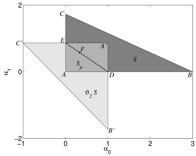
Figure 1: $SO(3)$-invariant Hermitian operators of trace $1$ for $3\otimes 3$ systems. Triangle $ABC$: The set $S$ of rotationally invariant density matrices. Triangle $A^{\prime}B^{\prime}C^{\prime}$: The transform $\vartheta_{2}S$. Rectangle $ADA^{\prime}E$: The set $S_{p}$ of PPT states, which is equal to the set $S_{s}$ of separable states (see Sec. V.3.2). The line $DE$ represents the fixed points of $\vartheta_{2}$, the point $F$ the state of maximal entropy and $B$ the singlet state $|00\rangle$.

The matrix $\Theta$ now becomes:

$$\Theta=\frac{1}{3}\left(\begin{array}[]{ccc}1&-\sqrt{3}&\sqrt{5}\\ -\sqrt{3}&\frac{3}{2}&\frac{\sqrt{15}}{2}\\ \sqrt{5}&\frac{\sqrt{15}}{2}&\frac{1}{2}\end{array}\right).$$ (58)

One easily verifies that this is a symmetric and orthogonal matrix of trace $1$. On eliminating the parameter $\alpha_{2}$ we find that $\vartheta_{2}$ acts as follows on the vertices of $S$:

$$A=\left(0,0\right) \mapsto A^{\prime}=\left(1,\frac{\sqrt{3}}{2}\right),$$ (59)

$$B=\left(3,0\right) \mapsto B^{\prime}=(1,-\sqrt{3}),$$ (60)

$$C=(0,\sqrt{3}) \mapsto C^{\prime}=\left(-1,\frac{\sqrt{3}}{2}\right).$$ (61)

Thus, $\vartheta_{2}S$ is the triangle with vertices $A^{\prime}$, $B^{\prime}$ and $C^{\prime}$.

The sets $S$ and $\vartheta_{2}S$ are depicted in Fig. 1. The figure also shows the line of the fixed points of $\vartheta_{2}$ with endpoints $D=(1,0)$ and $E=\left(0,\frac{\sqrt{3}}{2}\right)$. This line is easily determined from the matrix $\Theta$ and its eigenvectors. Being invariant under $\vartheta_{2}$, the point $F$, which describes the state of maximal entropy, lies of course on this line.

The rectangle with vertices $A$, $D$, $A^{\prime}$ and $E$ represents the intersection $S_{p}=S\cap\vartheta_{2}S$ of the PPT states. It should be noted that the rotational invariance in the present example is equivalent to the invariance under the product transformations $O\otimes O$, where $O$ varies over the group of orthogonal $3\times 3$ matrices VOLLBRECHT .

IV.2.3 $4\otimes 4$ systems

The case $N=4$ corresponds to a system composed of two particles with spin $j=\frac{3}{2}$. The total angular momentum assumes the values $J=0,1,2,3$. Thus we get a three-dimensional parameter space with parameters $(\alpha_{0},\alpha_{1},\alpha_{2})$. By virtue of Eq. (54) the set of rotationally invariant states is determined by the inequalities:

$$\frac{1}{4}\alpha_{0}+\frac{\sqrt{3}}{4}\alpha_{1}+\frac{\sqrt{5}}{4}\alpha_{2}\leq 1,\qquad\alpha_{0},\alpha_{1},\alpha_{2}\geq 0.$$ (62)

This shows that $S$ is a tetrahedron (3-simplex) with vertices $A=(0,0,0)$, $B=\left(4,0,0\right)$, $C=\left(0,\frac{4}{\sqrt{3}},0\right)$ and $D=\left(0,0,\frac{4}{\sqrt{5}}\right)$.

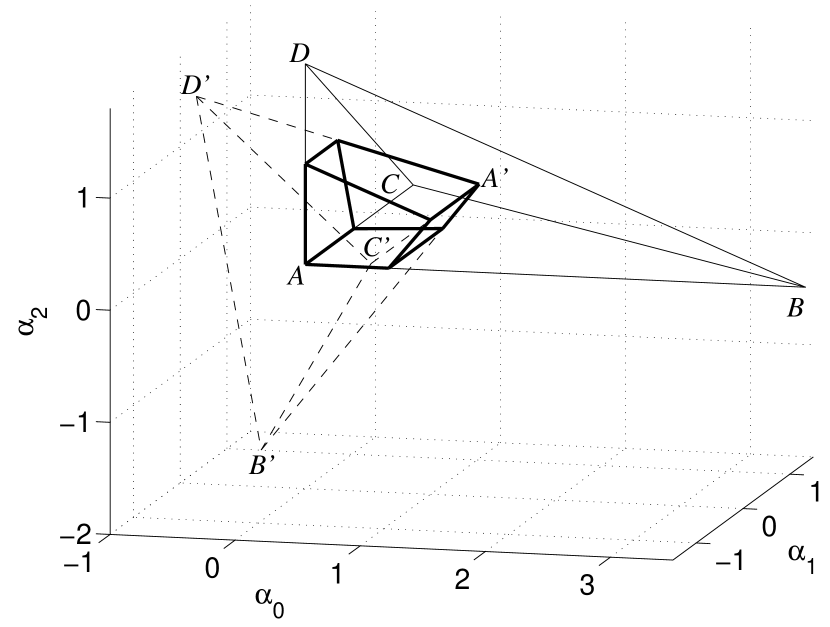
Figure 2: $SO(3)$-invariant Hermitian operators of trace $1$ for $4\otimes 4$ systems. The tetrahedron $ABCD$ (continuous lines) represents the set $S$ of invariant states, and the tetrahedron $A^{\prime}B^{\prime}C^{\prime}D^{\prime}$ (broken lines) its transform $\vartheta_{2}S$. The intersection (bold lines) is the set $S_{p}$ of the PPT states.

The matrix $\Theta$ is given by:

$$\Theta=\frac{1}{4}\left(\begin{array}[]{cccc}-1&\sqrt{3}&-\sqrt{5}&\sqrt{7}\\ \sqrt{3}&-\frac{11}{5}&\sqrt{\frac{3}{5}}&\frac{3\sqrt{21}}{5}\\ -\sqrt{5}&\sqrt{\frac{3}{5}}&3&\sqrt{\frac{7}{5}}\\ \sqrt{7}&\frac{3\sqrt{21}}{5}&\sqrt{\frac{7}{5}}&\frac{1}{5}\end{array}\right).$$ (63)

One checks that this matrix is symmetric, orthogonal and of trace zero. It leads to the following mapping of the vertices of the tetrahedron $S$ under $\vartheta_{2}$:

$$A=\left(0,0,0\right) \mapsto A^{\prime}=\left(1,\frac{3\sqrt{3}}{5},\frac{1}{\sqrt{5}}\right),$$ (64)

$$B=\left(4,0,0\right) \mapsto B^{\prime}=\left(-1,\sqrt{3},-\sqrt{5}\right),$$ (65)

$$C=\left(0,\frac{4}{\sqrt{3}},0\right) \mapsto C^{\prime}=\left(1,-\frac{11}{5\sqrt{3}},\frac{1}{\sqrt{5}}\right),$$ (66)

$$D=\left(0,0,\frac{4}{\sqrt{5}}\right) \mapsto D^{\prime}=\left(-1,\frac{\sqrt{3}}{5},\frac{3}{\sqrt{5}}\right).$$ (67)

The points $A^{\prime}$, $B^{\prime}$, $C^{\prime}$ and $D^{\prime}$ are the vertices of the transformed tetrahedron $\vartheta_{2}S$, as shown in Fig. 2.

We see from Fig. 2 that the intersection $S_{p}=S\cap\vartheta_{2}S$ is isomorphic to a 3-dimensional cube. An enlarged picture of this cube is shown in Fig. 3. The vertices of $S_{p}$ are given by the points $A$, $A^{\prime}$ and

$$E=\left(\frac{2}{3},0,0\right), E^{\prime}=\left(\frac{2}{3},\frac{2\sqrt{3}}{3},0\right),$$ (68)

$$F=\left(0,\frac{3\sqrt{3}}{5},0\right), F^{\prime}=\left(1,0,\frac{1}{\sqrt{5}}\right),$$ (69)

$$G=\left(0,0,\frac{2}{\sqrt{5}}\right), G^{\prime}=\left(0,\frac{2\sqrt{3}}{5},\frac{2}{\sqrt{5}}\right).$$ (70)

These points may be obtained as follows (see Fig. 3). One takes the three edges emerging from the vertex $A^{\prime}$ of the tetrahedron $\vartheta_{2}S$ and determines their intersection with the faces of the tetrahedron $S$. This yields the points $E^{\prime}$, $F^{\prime}$ and $G^{\prime}$. The points $E$, $F$ and $G$ are then given by the images of $E^{\prime}$, $F^{\prime}$ and $G^{\prime}$ under $\vartheta_{2}$.

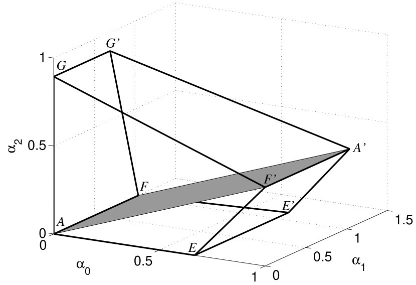
Figure 3: Enlarged picture of the cube $S_{p}$ of PPT states (see Fig. 2). The plane $AA^{\prime}FF^{\prime}$ subdivides $S_{p}$ into two prisms. The prism $AA^{\prime}FF^{\prime}GG^{\prime}$ represents the set $S_{s}$ of separable states (see Sec. V.3.3).

V Separable states

V.1 Construction of $SO(3)$-invariant separable states

The set of separable states is defined to be the set of states $\rho$ which can be written as a convex sum of product states:

$$\rho=\sum_{i}\lambda_{i}\rho_{i}^{(1)}\otimes\rho_{i}^{(2)},\qquad\lambda_{i}\geq 0,\qquad\sum_{i}\lambda_{i}=1,$$ (71)

where the $\rho_{i}^{(1)}$ and $\rho_{i}^{(2)}$ are normalized local states WERNER . It follows from this definition and from the positivity of $\vartheta$ that the map $\vartheta_{2}$ is positive on separable states. Thus, $\vartheta_{2}$ maps rotationally invariant and separable states to rotationally invariant and separable states.

We denote the set of $SO(3)$-invariant separable states by $S_{s}$. This set is contained in the set of states which are positive under $\vartheta_{2}$:

$$S_{s}\subset S_{p}=S\cap\vartheta_{2}S.$$ (72)

This equation expresses the Peres PPT criterion. It can easily be applied in the present formulation once the matrix $\Theta$ has been determined: Given a rotationally invariant state $\rho$ in terms of its parameter vector $\bm{\alpha}$ according to Eq. (4), a necessary condition for this state to be separable is that all components of the transformed parameter vector ${\bm{\alpha}}^{\prime}=\Theta{\bm{\alpha}}$ are positive.

To fully characterize the set of separable states one introduces a projection super-operator $\Pi$, also known as twirl operator. Given any state $\rho$ of the bipartite system the operator

$$\Pi\rho=\sum_{J=0}^{2j}\frac{1}{2J+1}P_{J}{\mbox{tr}}\{P_{J}\rho\}$$ (73)

is positive, of trace $1$ and rotationally invariant. The map $\rho\mapsto\Pi\rho$ defines a projection (i. e., $\Pi^{2}=\Pi$) from the total state space onto the space $S$ of rotationally invariant states. Moreover, if $\rho$ is separable then $\Pi\rho$ is again separable.

We see from Eq. (73) that the $\alpha_{J}$-parameters corresponding to the projection $\Pi\rho$ are given by $\alpha_{J}=\frac{N}{\sqrt{2J+1}}{\mathrm{tr}}\{P_{J}\rho\}$. If we take a pure product state

$$\rho=|\varphi^{(1)}\varphi^{(2)}\rangle\langle\varphi^{(1)}\varphi^{(2)}|$$ (74)

involving normalized local states $|\varphi^{(1)}\rangle$ and $|\varphi^{(2)}\rangle$, the $\alpha_{J}$-parameters of its projection are found to be

$$\alpha_{J}=\tilde{\alpha}_{J}[\varphi^{(1)},\varphi^{(2)}]=\frac{N}{\sqrt{2J+1}}\langle\varphi^{(1)}\varphi^{(2)}|P_{J}|\varphi^{(1)}\varphi^{(2)}\rangle.$$ (75)

It is known that any separable state can be written as a convex sum of pure product states. We define $W$ to be the range of the parameter vector $\bm{\alpha}$ whose components $\alpha_{J}$ are given by the above functionals $\tilde{\alpha}_{J}[\varphi^{(1)},\varphi^{(2)}]$, where $|\varphi^{(1)}\rangle$ and $|\varphi^{(2)}\rangle$ run independently over all normalized states in ${\mathcal{H}}$. With this definition one has the following result VOLLBRECHT : The set $S_{s}$ of rotationally invariant and separable states is equal to the convex hull of the range $W$, i. e., to the smallest convex set containing $W$. Thus, we have:

$$S_{s}={\mbox{hull}}(W)\subset S_{p}.$$ (76)

The determination of $S_{s}$ therefore amounts to the determination of the convex hull of the range of the functionals $\tilde{\alpha}_{J}[\varphi^{(1)},\varphi^{(2)}]$ given by Eq. (75). This task can be simplified by the following observations.

First, since $S_{s}$ is the convex hull of $W$ which, in turn, is contained in $S_{p}$, a good starting point is to consider the extreme points (vertices) of $S_{p}$. If one finds, for example, that all extreme points of $S_{p}$ belong to $W$ one concludes immediately that $S_{s}$ must be identical to $S_{p}$.

Second, it is clear by construction that the functionals $\tilde{\alpha}_{J}$ are invariant under simultaneous rotations $|\varphi^{(1,2)}\rangle\mapsto D(R)|\varphi^{(1,2)}\rangle$ of the input arguments. Pairs of state vectors differing by such a transformation are thus projected to one and the same point of the parameter space and need not be considered separately.

Third, the range $W$ is invariant under the map $\vartheta_{2}$. This means that if the point $\bm{\alpha}$ belongs to $W$, then also the transformed point $\Theta\bm{\alpha}$ belongs to $W$. This statement can easily be proven by use of the results of Sec. III.3. In fact, we have

$$\tilde{\alpha}_{J}[\varphi^{(1)},\tau\varphi^{(2)}] = \frac{N}{\sqrt{2J+1}}\langle\varphi^{(1)}\varphi^{(2)}|\vartheta_{2}P_{J}|\varphi^{(1)}\varphi^{(2)}\rangle$$ (77)

$$= \sum_{K=0}^{2j}\Theta_{JK}\tilde{\alpha}_{K}[\varphi^{(1)},\varphi^{(2)}].$$

We see that the transformation $\bm{\alpha}\mapsto\Theta\bm{\alpha}$ corresponds to the time reversal transformation $\tau$ carried out on the second input argument of the functionals. Equation (77) also demonstrates that if $|\varphi^{(2)}\rangle$ is invariant under $\tau$ the corresponding parameter vector represents, for any choice of $|\varphi^{(1)}\rangle$, a fixed point of $\Theta$.

V.2 Representation in terms of spherical tensors

In addition to the projections $P_{J}$ there exist further rotationally invariant operators which span the set $S$ and which lead to a particularly useful representation of the set of separable states. To construct these operators we introduce the irreducible spherical tensor operators $T_{JM}$ acting on ${\mathcal{H}}$, where, as before, $J=0,1,\ldots,2j$ and $M=-J,-J+1,\ldots,+J$. The matrix elements of these operators are defined by the $3$-$j$ symbols:

$$\langle jm|T_{JM}|jm^{\prime}\rangle=(-1)^{j-m}\sqrt{2J+1}\left(\begin{array}[]{ccc}j&j&J\\ m&-m^{\prime}&-M\end{array}\right).$$ (78)

According to the selection rules of the $3$-$j$ symbols the matrix element (78) is zero for $\Delta m\equiv m-m^{\prime}\neq M$. The tensor operators $T_{JM}$ represent a complete system of operators on ${\mathcal{H}}$ which are orthonormal with respect to the Hilbert-Schmidt inner product, i. e., one has ${\mathrm{tr}}\{T^{\dagger}_{JM}T_{J^{\prime}M^{\prime}}\}=\delta_{JJ^{\prime}}\delta_{MM^{\prime}}$.

For a fixed $J$ the $(2J+1)$ operators $T_{JM}$ transform according to an irreducible representation of the rotation group corresponding to the angular momentum $J$. For example, the $T_{1M}$ transform as the spherical components of a vector, while the $T_{2M}$ behave as the components of a second-rank tensor under rotations. For $N=2$ the tensor components $T_{1M}$ may be expressed in terms of the Pauli matrices as $T_{10}=\frac{1}{\sqrt{2}}\sigma_{3}$ and $T_{1,\pm 1}=\mp\frac{1}{2}(\sigma_{1}\pm i\sigma_{2})$. The definition (78) leads to the relation $T^{\dagger}_{JM}=T^{T}_{JM}=(-1)^{M}T_{J,-M}$. One concludes that the tensor operators are eigen-operators of the time reversal transformation: $\vartheta T_{JM}=(-1)^{J}T_{JM}$.

It follows from the transformation behaviour of the $T_{JM}$ that the operators on the product space defined by

$$Q_{J}=\sum_{M=-J}^{+J}T_{JM}\otimes T_{JM}^{\dagger}$$ (79)

are invariant under rotations. The connection between the projections $P_{J}$ and the operators $Q_{J}$ is provided by the relation

$$\vartheta_{2}P_{J}=Q_{J}{\mathbb{F}},$$ (80)

where we have introduced the flip operator ${\mathbb{F}}$ which is defined by

$${\mathbb{F}}|jm_{1}jm_{2}\rangle=|jm_{2}jm_{1}\rangle.$$ (81)

The proof of Eq. (80) is given in Appendix A.

Equation (80) leads to an alternative characterization of the set of separable states. Since $|\varphi^{(1)}\rangle$ and $|\varphi^{(2)}\rangle$ vary independently over all normalized states we may use the right-hand side of Eq. (77) instead of the original expression (75) for the functionals $\tilde{\alpha}_{J}[\varphi^{(1)},\varphi^{(2)}]$. If we introduce (80) into (77) we find that we can employ the functionals

$$\tilde{\alpha}_{J}[\varphi^{(1)},\varphi^{(2)}]=\frac{N}{\sqrt{2J+1}}\sum_{M=-J}^{+J}|\langle\varphi^{(1)}|T_{JM}|\varphi^{(2)}\rangle|^{2}$$ (82)

in order to construct the range $W$ and the set $S_{s}$ of separable states. An advantage of this formulation is that it leads to a very simple expression for $J=0$. Namely, since $T_{00}=\frac{1}{\sqrt{N}}I$ we have

$$\tilde{\alpha}_{0}[\varphi^{(1)},\varphi^{(2)}]=|\langle\varphi^{(1)}|\varphi^{(2)}\rangle|^{2}.$$ (83)

It might be interesting to note that Eq. (80) can be used to identify the one-parameter family of the Werner states given by

$$\rho_{W}=\frac{1}{N^{3}-N}\left[(N-\lambda)I\otimes I+(N\lambda-1){\mathbb{F}}\right],$$ (84)

where $-1\leq\lambda\leq+1$. These states are invariant under all product unitaries $U\otimes U$. Therefore, all states of the family are, in particular, invariant under rotations and belong to $S$. The parameters $\alpha^{W}_{J}$ corresponding to $\rho_{W}$ are found to be

$$\alpha^{W}_{J} = \frac{N}{\sqrt{2J+1}}{\mathrm{tr}}\{P_{J}\rho_{W}\}$$

$$= \frac{\sqrt{2J+1}}{N^{2}-1}\left[N-\lambda+(-1)^{2j+J}(N\lambda-1)\right].$$

To obtain this result one has to determine the expression ${\mathrm{tr}}\{P_{J}{\mathbb{F}}\}$. This may be done by noting that for $J=0$ Eq. (80) yields ${\mathbb{F}}=N\vartheta_{2}P_{0}$. The expression ${\mathrm{tr}}\{P_{J}{\mathbb{F}}\}$ can therefore be written in terms of the matrix elements $\Theta_{J0}$ which are given by Eq. (49). The family of the isotropic states can be embedded in a similar way into $S$ if one first performs the local unitary transformation $I\otimes V$.

V.3 Examples

We construct the set $S_{s}$ of separable states for the examples considered in Sec. IV.2. To this end, we make use of the functionals (82) which characterize $S_{s}$ and of the general properties of the range $W$ described in Sec. V.1.

V.3.1 $2\otimes 2$ systems

In the case of our first example discussed in Sec. IV.2.1 we found that the parameter $\alpha_{0}$ describes a PPT state if and only if $\alpha_{0}\in S_{p}=[0,1]$. We immediately see from Eq. (83) that the set of separable states and the set of PPT states are identical, that is $S_{s}=S_{p}$. In fact, according to Eq. (83) the functional $\tilde{\alpha}_{0}[\varphi^{(1)},\varphi^{(2)}]$ can take any value in the interval $[0,1]$ because $|\varphi^{(1,2)}\rangle$ are arbitrary normalized states. This shows that in the present case positivity under $\vartheta_{2}$ is a necessary and sufficient condition for separability, which is a well-known fact HORODECKI96b .

V.3.2 $3\otimes 3$ systems

Using the results of Sec. IV.2.2 we show that also for $3\otimes 3$ systems the set of PPT states and the set of separable states coincide, i. e., $S_{s}=S_{p}$. Thus, positivity under $\vartheta_{2}$ is again a necessary and sufficient condition for separability in this case, as has been demonstrated by Vollbrecht and Werner VOLLBRECHT . To prove this we verify that the extreme points of $S_{p}$, that is, the points $A$, $A^{\prime}$, $D$ and $E$ belong to the range $W$ (see Fig. 1).

First, we choose $|\varphi^{(1)}\rangle=|j=1,m=+1\rangle$ and $|\varphi^{(2)}\rangle=|j=1,m=-1\rangle$. These states are orthogonal and, hence, $\tilde{\alpha}_{0}=0$ according to Eq. (83). Using the selection rules for the matrix elements (78) of the tensor operators $T_{1M}$ one sees that also $\tilde{\alpha}_{1}=0$ (the operators $T_{1M}$ cannot connect states whose magnetic quantum numbers differ by $2$). This shows that $A=(0,0)$ belongs to the range $W$. It also follows that $A^{\prime}$ belongs to $W$, because $A^{\prime}$ is the image of $A$ under $\vartheta_{2}$.

Next, we consider the state

$$|\varphi^{(2)}\rangle=\frac{1}{\sqrt{2}}(|1,+1\rangle+|1,-1\rangle).$$ (86)

This state is invariant under the time reversal transformation (20). Thus, for any choice of $|\varphi^{(1)}\rangle$, the point $(\tilde{\alpha}_{0},\tilde{\alpha}_{1})$ is a fixed point of $\vartheta_{2}$ and, hence, belongs to the line $DE$ (see Fig. 1). If $|\varphi^{(1)}\rangle$ is any state orthogonal to $|\varphi^{(2)}\rangle$ we have that, additionally, $\tilde{\alpha}_{0}=0$ and, hence, $(\tilde{\alpha}_{0},\tilde{\alpha}_{1})=\left(0,\frac{\sqrt{3}}{2}\right)\equiv E\in W$. One the other hand, if we take $|\varphi^{(1)}\rangle=|\varphi^{(2)}\rangle$, then $\tilde{\alpha}_{0}=1$ and, therefore, $(\tilde{\alpha}_{0},\tilde{\alpha}_{1})=(1,0)\equiv D\in W$. This concludes the proof.

V.3.3 $4\otimes 4$ systems

For $4\otimes 4$ systems it is again possible to give a complete geometric construction of the set of separable states by use of the results of Sec. IV.2.3. In the case $N=4$ we have to consider the following functionals:

$$\tilde{\alpha}_{0}[\varphi^{(1)},\varphi^{(2)}]\! = \!|\langle\varphi^{(1)}|\varphi^{(2)}\rangle|^{2},$$ (87)

$$\tilde{\alpha}_{1}[\varphi^{(1)},\varphi^{(2)}]\! = \!\frac{4}{\sqrt{3}}\sum_{M=-1}^{+1}|\langle\varphi^{(1)}|T_{1M}|\varphi^{(2)}\rangle|^{2},$$ (88)

$$\tilde{\alpha}_{2}[\varphi^{(1)},\varphi^{(2)}]\! = \!\frac{4}{\sqrt{5}}\sum_{M=-2}^{+2}|\langle\varphi^{(1)}|T_{2M}|\varphi^{(2)}\rangle|^{2}.$$ (89)

To construct $S_{s}$ we proceed in four steps, investigating the extreme points of $S_{p}$ given by Eqs. (64), (68), (69) and (70) (see Fig. 3).

(1) We show that $A,A^{\prime}\in W$. To proof this we take $|\varphi^{(1)}\rangle=|\frac{3}{2},+\frac{3}{2}\rangle$ and $|\varphi^{(2)}\rangle=|\frac{3}{2},-\frac{3}{2}\rangle$. These states are orthogonal and, therefore, $\tilde{\alpha}_{0}=0$ according to Eq. (87). Since the magnetic quantum numbers of the states differ by $3$ the selection rules for the matrix elements (78) yield that $\langle\varphi^{(1)}|T_{JM}|\varphi^{(2)}\rangle=0$ for $J=1,2$. Thus, Eqs. (88) and (89) yield $\tilde{\alpha}_{1}=\tilde{\alpha}_{2}=0$. Hence, $A=(0,0,0)$ and $A^{\prime}=\vartheta_{2}A$ belong to $W$.

(2) We demonstrate that also $G,G^{\prime}\in W$. To this end, we take $|\varphi^{(1)}\rangle=|\frac{3}{2},+\frac{3}{2}\rangle$ and $|\varphi^{(2)}\rangle=|\frac{3}{2},-\frac{1}{2}\rangle$. These states are again orthogonal and we get $\tilde{\alpha}_{0}=0$. Since $\Delta m=2$ the matrix elements $\langle\varphi^{(1)}|T_{1M}|\varphi^{(2)}\rangle$ vanish and, therefore, $\tilde{\alpha}_{1}=0$. The only matrix element of the $T_{2M}$ which is not equal to zero on account of the selection rules is given by

$$\langle\varphi^{(1)}|T_{22}|\varphi^{(2)}\rangle=\frac{1}{\sqrt{2}}.$$ (90)

Thus, with the help of Eq. (89) we obtain $\tilde{\alpha}_{2}=\frac{2}{\sqrt{5}}$. One concludes that $G=(0,0,\frac{2}{\sqrt{5}})$ and, hence, also $G^{\prime}=\vartheta_{2}G$ belong to $W$.

(3) We claim that $F,F^{\prime}\in W$. To prove this we choose the states:

$$|\varphi^{(1)}\rangle = \frac{1}{\sqrt{2}}\left(\left|\frac{3}{2},+\frac{3}{2}\right\rangle+\left|\frac{3}{2},-\frac{3}{2}\right\rangle\right),$$ (91)

$$|\varphi^{(2)}\rangle = \frac{1}{\sqrt{2}}\left(\left|\frac{3}{2},+\frac{3}{2}\right\rangle-\left|\frac{3}{2},-\frac{3}{2}\right\rangle\right).$$ (92)

These states are obviously orthogonal and we get again $\tilde{\alpha}_{0}=0$. The selection rules now yield $\langle\varphi^{(1)}|T_{JM}|\varphi^{(2)}\rangle=0$ for $J=1,2$ and $M\neq 0$, while

$$\langle\varphi^{(1)}|T_{J0}|\varphi^{(2)}\rangle = \frac{1}{2}\left\langle\frac{3}{2},+\frac{3}{2}\right|T_{J0}\left|\frac{3}{2},+\frac{3}{2}\right\rangle$$ (93)

$$- \frac{1}{2}\left\langle\frac{3}{2},-\frac{3}{2}\right|T_{J0}\left|\frac{3}{2},-\frac{3}{2}\right\rangle.$$

We have the following general relation between the matrix elements of the tensor operators:

$$\langle j,-m|T_{J0}|j,-m\rangle=(-1)^{J}\langle j,+m|T_{J0}|j,+m\rangle.$$ (94)

On using this we see that the expression (93) vanishes for $J=2$. It follows that $\tilde{\alpha}_{2}=0$. On the other hand, for $J=1$ we obtain

$$\langle\varphi^{(1)}|T_{10}|\varphi^{(2)}\rangle=\left\langle\frac{3}{2},+\frac{3}{2}\right|T_{10}\left|\frac{3}{2},+\frac{3}{2}\right\rangle=\frac{3}{2\sqrt{5}}.$$ (95)

With the help of (88) this leads to $\tilde{\alpha}_{1}=\frac{3\sqrt{3}}{5}$. In summary, we see that $F=(0,\frac{3\sqrt{3}}{5},0)$ and $F^{\prime}=\vartheta_{2}F$ belong to the range $W$.

(4) It is shown in Appendix B that the functionals (87) and (89) fulfill the inequality:

$$\tilde{\alpha}_{2}[\varphi^{(1)},\varphi^{(2)}]\geq\frac{1}{\sqrt{5}}\tilde{\alpha}_{0}[\varphi^{(1)},\varphi^{(2)}].$$ (96)

It follows that $E$ and $E^{\prime}$ do not belong to the range $W$. Namely, for these points we must have $\tilde{\alpha}_{2}=0$ and $\tilde{\alpha}_{0}=\frac{2}{3}$ [see Eq. (68)] which contradicts the inequality (96). This shows that in the present case $S_{s}$ is a true subset of $S_{p}$, i. e., positivity under $\vartheta_{2}$ is a necessary but not sufficient condition for separability.

According to Sec. IV.2.3 the set $S_{s}$ of separable states is contained in the cube $S_{p}$ of the PPT states (see Fig. 3). By the above results the points $A$, $A^{\prime}$, $F$, $F^{\prime}$, $G$, and $G^{\prime}$ are contained in the range $W$. Since $S_{s}$ is the convex hull of $W$ we conclude that $S_{s}$ contains at least the polyhedron $AA^{\prime}FF^{\prime}GG^{\prime}$. We observe that this polyhedron is isomorphic to a prism.

The inequality (96) yields an additional condition for the separable states. It implies that all points of the range $W$ must lie on or above the plane which is defined by $\alpha_{2}=\frac{1}{\sqrt{5}}\alpha_{0}$ and which is indicated as gray surface in Fig. 3. We note that according to Eqs. (64) and (69) the points $A$, $A^{\prime}$, $F$ and $F^{\prime}$ belong to this plane. It follows that the set $S_{s}$ of separable states is in fact identical to the prism $AA^{\prime}FF^{\prime}GG^{\prime}$.

In summary, the convex structure of the set of $SO(3)$-invariant states of $4\otimes 4$ systems may be described by the following inclusions:

$$(\mbox{prism}\;S_{s})\subset(\mbox{cube}\;S_{p})\subset(\mbox{tetrahedron}\;S).$$ (97)

The tetrahedron $S$, representing the set of all invariant states, decomposes into the cube $S_{p}$ of PPT states and the set $S\setminus S_{p}$ of entangled states whose partial transposition has negative eigenvalues. The cube $S_{p}$ of PPT states, in turn, consists of the prism $S_{s}$ of separable states and of the set $S_{p}\setminus S_{s}$ of entangled PPT states. The plane $\alpha_{2}=\frac{1}{\sqrt{5}}\alpha_{0}$ thus separates the entangled PPT states from the separable states.

As can be seen from Fig. 3 the set $S_{p}\setminus S_{s}$ is isomorphic to a prism from which one face has been removed. All states belonging to this set are inseparable and have positive partial transposition. This leads to the important conclusion that $S_{p}\setminus S_{s}$ represents a three-dimensional manifold of bound entangled states, i. e., states which cannot be distilled by local quantum operations and classical communication BENNETT ; VINCENZO ; HORODECKI98 .

VI Discussion and conclusions

We have analyzed the structure of the state spaces of bipartite $N\otimes N$ systems which are invariant under product representations of the rotation group. The main tool of the analysis is the positive map $\vartheta$ which is unitarily equivalent to the transposition $T$ and describes the behaviour of local states under time reversal. Employing the properties of $\vartheta$ one relates the partial time reversal $\vartheta_{2}=I\otimes\vartheta$ to a linear transformation of the parameter space ${\mathbb{R}}^{N}=\{\bm{\alpha}\}$ and expresses the corresponding matrix $\Theta$ in terms of Wigner’s $6$-$j$ symbols. This matrix has been used to obtain geometrical representations for the sets of the separable and of the PPT states in the cases $N=2$, $3$ and $4$.

In Sec. V.3.3 the inequality (96) enabled the construction of the set of separable states. Taken together with the Peres PPT criterion this inequality yields a necessary and sufficient condition for the separability of rotationally invariant states of $4\otimes 4$ systems. It is of great interest to examine the possibility of an extension of this picture to higher dimensions. In this context it is important to observe that the inequality (96) expresses the positivity of a certain map $\Phi$ which is given by

$$\Phi B=\sum_{M=-2}^{+2}T_{2M}BT_{2M}^{\dagger}-T_{00}BT_{00}^{\dagger}.$$ (98)

This map is non-decomposable and detects all entangled PPT states. Hence, we need exactly two maps, namely $\vartheta$ and $\Phi$, in order to identify uniquely all separable states. These maps yield complementary conditions for separability in the sense that the two inequalities

$$(I\otimes\vartheta)\rho\geq 0\qquad{\mbox{and}}\qquad(I\otimes\Phi)\rho\geq 0$$ (99)

constitute a necessary and sufficient separability criterion. It should also be noted that the proof of Appendix B does not rely on any invariance requirement. We conclude that positivity under the map $\Phi_{2}=I\otimes\Phi$ is a necessary condition of separability for all (not necessarily rotationally invariant) states of $4\otimes 4$ systems.

The positive map introduced in Eq. (98) corresponds to an entanglement witness HORODECKI96a ; TERHAL ; LEWENSTEIN00 which is given by the operator ${\mathcal{W}}=P_{2}-P_{0}$. The plane $\alpha_{2}=\frac{1}{\sqrt{5}}\alpha_{0}$ in parameter space may be viewed as an optimal hyperplane defined by this witness ${\mathcal{W}}$. This fact leads to the following interpretation of the inequality (96): If a measurement of the total angular momentum is carried out on a separable state, the probability of finding the value $J=2$ must be larger or equal to the probability of finding the value $J=0$.

The method developed here suggests many generalizations and applications. An obvious extension is to consider bipartite systems whose local state spaces are not isomorphic, involving two different angular momenta $j^{(1)}\neq j^{(2)}$. Further important topics are an extension of the analysis given in Sec. V.3 to higher-dimensional systems, the treatment of other symmetry groups, and entanglement in multipartite systems.

The matrix $\Theta$ contains the complete information on the behaviour of the spectrum of the invariant states under partial transposition. It can also be used to express various separability criteria and entanglement measures and to design positive maps and entanglement witnesses. Examples of applications are the determination of the relative entropy of entanglement with respect to the set of PPT states AUDENAERT , and the entanglement measure given by the negativity VIDAL ; EISERT . The negativity, for instance, is determined by the trace norm of the partially time-reversed state which can be written as

$$||\vartheta_{2}\rho||_{1}=\sum_{J}\frac{\sqrt{2J+1}}{N}\left|\sum_{K}\Theta_{JK}\alpha_{K}\right|,$$ (100)

where $||A||_{1}={\mathrm{tr}}|A|$ denotes the trace norm of $A$.

In Refs. HORODECKI99 ; CERF a necessary separability criterion, the reduction criterion, has been introduced which is based on the positive map defined by $\Lambda B=I{\mathrm{tr}}B-B$. This criterion is not stronger than the Peres criterion, but has the important benefit that any state violating it can be distilled. For $SO(3)$-invariant states the reduction criterion is equivalent to the inequality based on the quantum Rényi entropy $S_{\infty}$ HORODECKI96b ; HORODECKI99 and to the disorder criterion KEMPE , and takes the form $\frac{1}{N}I\otimes I-\rho\geq 0$. In terms of the parameters $\alpha_{J}$ this can be expressed through $\alpha_{J}\leq\sqrt{2J+1}$. We see explicitly from our examples that for rotationally invariant states the reduction criterion is in fact much weaker than the Peres criterion. For instance, in the case $N=4$ we get from it the conditions $\alpha_{0}\leq 1$ and $\alpha_{1}\leq\sqrt{3}$. The region defined by these inequalities is much larger than $S_{p}$ and than the true set $S_{s}$ of separable states (see Fig. 3).

Recently, a necessary criterion for separability has been developed by Rudolph RUDOLPH02 ; RUDOLPH03 , which is known as cross norm or realignment criterion CHEN . This criterion is based on the cross norm of the states of the tensor product space RUDOLPH00 and provides strong conditions for separability. It is generally neither weaker nor stronger than the PPT criterion. It can detect, however, bound entanglement. To formulate the cross norm criterion we associate with any density matrix $\rho=\sum_{i}C_{i}\otimes D_{i}$ a map $\Phi_{\rho}$ by means of the formula

$$\Phi_{\rho}B=\sum_{i}C_{i}{\mathrm{tr}}\{(\vartheta D_{i})B\}.$$ (101)

For a separable state $\rho$ the corresponding map $\Phi_{\rho}$ is a contraction with respect to the trace norm, i. e., we have $||\Phi_{\rho}||_{1}\leq 1$, which immediately yields a necessary condition for separability.

The application of the cross norm criterion to rotationally invariant states leads to an inequality which can again be expressed entirely in terms of the elements of the matrix $\Theta$. If the state $\rho$ is given by its parameters $\alpha_{J}$ the trace norm of $\Phi_{\rho}$ can be written in a form analogous to Eq. (100):

$$||\Phi_{\rho}||_{1}=\sum_{J}\frac{\sqrt{2J+1}}{N}\left|\sum_{K}\Theta_{JK}(-1)^{K}\alpha_{K}\right|\leq 1.$$ (102)

This is a general expression for the cross norm criterion of $SO(3)$-invariant states in any dimension $N$. It allows an explicit determination of the regions in parameter space satisfying or violating the criterion. In particular, with the help of the above formula one immediately evaluates the trace norm $||\Phi_{\rho}||_{1}$ for the families of the Werner states and of the isotropic states.

We finally mention that the present results could also find a number of important applications in the theory of open systems TheWork . The close connection to open system is based on an isomorphism JAMIOLKOWSKI between states $\rho$ on the tensor product space ${\mathcal{H}}\otimes{\mathcal{H}}$ and completely positive maps $\Phi$ of operators on ${\mathcal{H}}$. We define this isomorphism by the relation $\rho=(I\otimes\Phi)P_{0}$. Apart from a normalization factor this relation is equivalent to Eq. (101). It yields a one-to-one correspondence between the rotationally invariant density matrices $\rho$ and the completely positive maps $\Phi$ which are trace-preserving and rotationally invariant. Such maps arise through the interaction of open systems with isotropic environments. The isomorphism thus allows one to use the structure of $S$ in the construction of appropriate representations of one-parameter families of quantum dynamical maps and to derive the general form of isotropic non-Markovian quantum processes.

Appendix A Proof of relation (80)

In the basis of the product states $|m_{1}m_{2}\rangle\equiv|jm_{1}jm_{2}\rangle$ the matrix elements of the operator $\vartheta_{2}P_{J}$ are found to be

$$\langle m_{1}m_{2}|\vartheta_{2}P_{J}|m^{\prime}_{1}m^{\prime}_{2}\rangle$$ (103)

$$=(-1)^{2j-m_{2}-m^{\prime}_{2}}\langle m_{1},-m^{\prime}_{2}|P_{J}|m^{\prime}_{1},-m_{2}\rangle,$$

where we have used the definition (9) of the $\vartheta_{2}$-transformation as well as the matrix elements (16) of the unitary matrix $V$ introduced in Eq. (15). On the other hand, the definition (78) of the tensor operators and Eq. (32) lead to

$$\langle m|T_{JM}|m^{\prime}\rangle = (-1)^{j-m^{\prime}}\langle m,-m^{\prime}|JM\rangle,$$ (104)

$$\langle m|T^{\dagger}_{JM}|m^{\prime}\rangle = (-1)^{j-m}\langle m^{\prime},-m|JM\rangle.$$ (105)

We recall that the matrix elements on the right-hand sides are vector-coupling coefficients which are taken to be real following the usual phase conventions. The definitions (79) and (81) for the operators $Q_{J}$ and for the flip operator ${\mathbb{F}}$ yield:

$$\langle m_{1}m_{2}|Q_{J}{\mathbb{F}}|m^{\prime}_{1}m^{\prime}_{2}\rangle$$ (106)

$$=\sum_{M=-J}^{+J}(-1)^{2j-m_{2}-m^{\prime}_{2}}\langle m_{1},-m^{\prime}_{2}|JM\rangle\langle JM|m^{\prime}_{1},-m_{2}\rangle$$

$$=(-1)^{2j-m_{2}-m^{\prime}_{2}}\langle m_{1},-m^{\prime}_{2}|P_{J}|m^{\prime}_{1},-m_{2}\rangle.$$

Comparing this with (103) we see that $Q_{J}{\mathbb{F}}=\vartheta_{2}P_{J}$, as claimed.

Appendix B Proof of inequality (96)

We take any fixed normalized state $|\varphi^{(2)}\rangle$ and decompose it with respect to the basis states $|m\rangle\equiv|jm\rangle$:

$$|\varphi^{(2)}\rangle=c_{1}\left|+\frac{3}{2}\right\rangle+c_{2}\left|+\frac{1}{2}\right\rangle+c_{3}\left|-\frac{1}{2}\right\rangle+c_{4}\left|-\frac{3}{2}\right\rangle.$$ (107)

The normalization condition for the amplitudes $c_{i}$ reads

$$\sum_{i=1}^{4}|c_{i}|^{2}=1.$$ (108)

Consider then the operator:

$$A=\frac{4}{\sqrt{5}}\sum_{M=-2}^{+2}T_{2M}|\varphi^{(2)}\rangle\langle\varphi^{(2)}|T^{\dagger}_{2M}.$$ (109)

This operator is obviously Hermitian and positive and we have $\tilde{\alpha}_{2}[\varphi^{(1)},\varphi^{(2)}]=\langle\varphi^{(1)}|A|\varphi^{(1)}\rangle$. It will be demonstrated below that $|\varphi^{(2)}\rangle$ is an eigenvector of $A$ corresponding to the eigenvalue $\frac{1}{\sqrt{5}}$:

$$A|\varphi^{(2)}\rangle=\frac{1}{\sqrt{5}}|\varphi^{(2)}\rangle.$$ (110)

This equation implies that $A$ can be written as

$$A=\tilde{A}+\frac{1}{\sqrt{5}}|\varphi^{(2)}\rangle\langle\varphi^{(2)}|,$$ (111)

where $\tilde{A}$ is again a positive operator. This leads to:

$$\tilde{\alpha}_{2}[\varphi^{(1)},\varphi^{(2)}] = \langle\varphi^{(1)}|\tilde{A}|\varphi^{(1)}\rangle+\frac{1}{\sqrt{5}}|\langle\varphi^{(1)}|\varphi^{(2)}\rangle|^{2}$$ (112)

$$\geq \frac{1}{\sqrt{5}}\tilde{\alpha}_{0}[\varphi^{(1)},\varphi^{(2)}],$$

which proves the inequality (96).

It remains to demonstrate the eigenvector relation (110). To this end, we determine the matrix representation of the operator $A$ in the basis $|m\rangle$. With the help of the matrix elements (78) of the tensor operators $T_{JM}$ one finds that $A$ is represented by the matrix

$$A=\frac{1}{\sqrt{5}}\left[\begin{array}[]{cccc}|c_{1}|^{2}+2|c_{2}|^{2}+2|c_{3}|^{2}&-c_{1}c_{2}^{*}+2c_{3}c_{4}^{*}&-c_{1}c_{3}^{*}-2c_{2}c_{4}^{*}&c_{1}c_{4}^{*}\\ -c_{1}^{*}c_{2}+2c_{3}^{*}c_{4}&|c_{2}|^{2}+2|c_{1}|^{2}+2|c_{4}|^{2}&c_{2}c_{3}^{*}&-c_{2}c_{4}^{*}-2c_{1}c_{3}^{*}\\ -c_{1}^{*}c_{3}-2c_{2}^{*}c_{4}&c_{2}^{*}c_{3}&|c_{3}|^{2}+2|c_{4}|^{2}+2|c_{1}|^{2}&-c_{3}c_{4}^{*}+2c_{1}c_{2}^{*}\\ c_{1}^{*}c_{4}&-c_{2}^{*}c_{4}-2c_{1}^{*}c_{3}&-c_{3}^{*}c_{4}+2c_{1}^{*}c_{2}&|c_{4}|^{2}+2|c_{3}|^{2}+2|c_{2}|^{2}\\ \end{array}\right].$$ (113)

It is now easy to verify by an explicit calculation that the vector $c=(c_{1},c_{2},c_{3},c_{4})^{T}$, which represents the state $|\varphi^{(2)}\rangle$ according to Eq. (107), is an eigenvector of this matrix corresponding to the eigenvalue $\frac{1}{\sqrt{5}}$. This concludes the proof.

References

- (1) R. F. Werner, Phys. Rev. A 40, 4277 (1989).
- (2) K. Eckert, O. Gühne, F. Hulpke, P. Hyllus, J. Korbicz, J. Mompart, D. Bruß, M. Lewenstein, A. Sanpera, in Quantum Information Processing, edited by G. Leuchs and T. Beth (Wiley-VCH, Berlin, 2005).
- (3) M. A. Nielsen, J. Phys. A: Math. Gen. 34, 6987 (2001).
- (4) G. Alber, T. Beth, M. Horodecki, P. Horodecki, R. Horodecki, M. Rötteler, H. Weinfurter, R. Werner, A. Zeilinger, Quantum Information (Springer-Verlag, Berlin, 2001).
- (5) M. A. Nielsen and I. L. Chuang, Quantum Computation and Quantum Information (Cambridge University Press, Cambridge, 2000).
- (6) K. G. H. Vollbrecht, R. F. Werner, Phys. Rev. A 64, 062307 (2001).
- (7) A. J. Bracken, Phys. Rev. A 69, 052331 (2004).
- (8) M. Horodecki, P. Horodecki, Phys. Rev. A 59, 4206 (1999).
- (9) E. M. Rains, Phys. Rev. A 60, 179 (1999).
- (10) S. L. Woronowicz, Rep. Math. Phys. 10, 165 (1976).
- (11) M. Horodecki, P. Horodecki, R. Horodecki, Phys. Rev. Lett. 80, 5239 (1998).
- (12) A. Peres, Phys. Rev. Lett. 77, 1413 (1996).
- (13) E. P. Wigner, Group theory and its application to the quantum mechanics of atomic spectra (Academic Press, New York, 1959).
- (14) A. R. Edmonds, Angular Momentum in Quantum Mechanics (Princeton University Press, Princeton, 1957).
- (15) W. F. Stinespring, Proc. Amer. Math. Soc. 6, 211 (1955).
- (16) M.-D. Choi, Can. J. Math. 24, 520 (1972).
- (17) M.-D. Choi, Linear Algebr. Appl. 10, 285 (1975).
- (18) K. Kraus, States, Effects, and Operations, Vol. 190 of Lecture Notes in Physics (Springer-Verlag, Berlin, 1983).
- (19) K. Kraus, Ann. Phys. (N.Y.) 64, 311 (1971).
- (20) M. Horodecki, P. Horodecki, R. Horodecki, Phys. Lett. A 223, 1 (1996).
- (21) A. Sanpera, R. Tarrach, G. Vidal, e-print eprint quant-ph/9707041.
- (22) P. Busch, P. J. Lathi, Found. Phys. 20, 1429 (1990).
- (23) R. Horodecki, M. Horodecki, Phys. Rev. A 54, 1838 (1996).
- (24) C. H. Bennett, G. Brassard, S. Popescu, B. Schumacher, J. A. Smolin, W. K. Wootters, Phys. Rev. Lett. 76, 722 (1996).
- (25) C. H. Bennett, D. P. DiVincenzo, J. A. Smolin, W. K. Wootters, Phys. Rev. A 54, 3824 (1996).
- (26) B. M. Terhal, Phys. Lett. A 271, 319 (2000).
- (27) M. Lewenstein, B. Kraus, J. I. Cirac, P. Horodecki, Phys. Rev. A 62, 052310 (2000).
- (28) K. Audenaert, B. De Moor, K. G. H. Vollbrecht, R. F. Werner, Phys. Rev. A 66, 032310 (2002).
- (29) G. Vidal, R. F. Werner, Phys. Rev. A 65, 032314 (2002).
- (30) K. Audenaert, M. B. Plenio, J. Eisert, Phys. Rev. Lett. 90, 027901 (2003).
- (31) N. J. Cerf, C. Adami, R. M. Gingrich, Phys. Rev. A 60, 898 (1999).
- (32) M. A. Nielsen, J. Kempe, Phys. Rev. Lett. 86, 5184 (2001).
- (33) O. Rudolph, e-print eprint quant-ph/0202121.
- (34) O. Rudolph, Phys. Rev. A 67, 032312 (2003).
- (35) Kai Chen, Ling-An Wu, Quant. Inf. Comp. 3, 193 (2003).
- (36) O. Rudolph, J. Phys. A: Math. Gen. 33, 3951 (2000).
- (37) H. P. Breuer and F. Petruccione, The Theory of Open Quantum Systems (Oxford University Press, Oxford, 2002).
- (38) A. Jamiolkowski, Rep. Math. Phys. 3, 275 (1972).