On the limit cycle for the $1/r^{2}$ potential in momentum space

Abstract

The renormalization of the attractive $1/r^{2}$ potential has recently been studied using a variety of regulators. In particular, it was shown that renormalization with a square well in position space allows multiple solutions for the depth of the square well, including, but not requiring a renormalization group limit cycle. Here, we consider the renormalization of the $1/r^{2}$ potential in momentum space. We regulate the problem with a momentum cutoff and absorb the cutoff dependence using a momentum-independent counterterm potential. The strength of this counterterm is uniquely determined and runs on a limit cycle. We also calculate the bound state spectrum and scattering observables, emphasizing the manifestation of the limit cycle in these observables.

I Introduction

The renormalization of the quantum mechanical $1/r^{2}$ potential has attracted some interest recently because this singular potential is one of the simplest examples displaying discrete scale invariance and a renormalization group limit cycle Beane:2000wh ; Bawin:2003dm ; Braaten:2004pg ; Barford:2004fz .

The renormalization group (RG) is an important tool in many areas of modern physics Wilson:dy . Its applications range from critical phenomena in condensed matter physics to the renormalization of quantum field theories in nuclear and particle physics. The solutions of the RG can have many different topologies. Most applications, however, involve a renormalization group flow towards a (scale invariant) fixed point. A prominent example is Quantum Chromodynamics (QCD) the theory of the strong interactions. QCD has a single coupling constant $\alpha_{s}(\Lambda)$ with an asymptotically free ultraviolet fixed point: $\alpha_{s}(\Lambda)\to 0$ as the momentum cutoff $\Lambda$ is taken to infinity Gross:1973id ; Politzer:fx .

The possibility of an RG limit cycle was already pointed out by Wilson in 1971 Wilson:1970ag . A limit cycle is a closed curve in the space of coupling constants that is invariant under the RG flow. The RG flow completes a cycle around the curve every time the cutoff is changed by a multiplicative factor $\lambda_{0}$. This number $\lambda_{0}$ is called the preferred scaling factor. A limit cycle requires at least two coupling constants coupled by the RG equations if the couplings are continuous Wilson:1970ag . With a single coupling constant, a limit cycle can only occur if the coupling has discontinuities. A necessary condition for a limit cycle is invariance under discrete scale transformations: $x\to\lambda_{0}^{n}x$, where $n$ is an integer. This discrete scaling symmetry is reflected in log-periodic behavior of physical observables. It is interesting to observe that discrete scale invariance also arises in a variety of other contexts such as turbulence, sandpiles, earthquakes, and financial crashes Sor97 . We also note that because of the $c$-theorem in two spatial dimensions Zamolodchikov:gt , limit cycles are expected to occur only in $D\geq 3$ dimensions.

One important example of a limit cycle that was identified long ago from its manifestation in the bound state spectrum, is the three-body problem with large scattering length $a$ Albe-81 . In the limit $a\to\pm\infty$, there is an accumulation of 3-body bound states near threshold with binding energies differing by multiplicative factors of $\lambda_{0}^{2}\simeq 515.03$ Efimov70 . This phenomenon – the Efimov effect – can be understood in terms of a renormalization group limit cycle with discrete scaling factor $\lambda_{0}\simeq 22.7$.

The three-body problem with large $a$ is intimately connected to the quantum-mechanical $1/r^{2}$ potential. In the ultraviolet limit of large three-momenta, the three-body problem can be mapped into a one-dimensional Schrödinger equation with a $1/\rho^{2}$ potential where $\rho^{2}=r_{12}^{2}+r_{13}^{2}+r_{23}^{2}$ is the hyperradius of the three particles ($r_{ij}\equiv|{\bm{r}}_{i}-{\bm{r}}_{j}|$) Efi71 . As a consequence, the renormalization of both problems is similar.

In the effective field theory (EFT) formulation of the three-body problem with large scattering length, the limit cycle is evident in the RG evolution of a contact three-body interaction which is required for renormalization at leading order in the EFT expansion Bedaque:1998kg ; BHvK99b . The limit cycle behavior has important consequences in nuclear and atomic three-body systems BrH04 . For example, it has been conjectured that QCD has an infrared RG limit cycle at special values of the quark masses Braaten:2003dw . Limit cycles have recently also been realized in discrete Hamiltonian models Glazek:2002hq ; Glazek:2004 , superconductivity LeClair:2002ux ; Anfoss05 , quantum field theory models Leclair:2003xj ; Bernard:2001sc , and S-matrix models LeClair:2003hj ; LeClair:2004ps .

Since discrete scale invariance occurs in a wide variety of complex systems Sor97 , RG limit cycles may play a more important role in physics than previously realized. In this context, the study of the attractive $1/r^{2}$ potential sheds some light on the general properties of limit cycles and the mechanism of their emergence. Furthermore, many properties of the EFT approach to the three-body system with large $a$ can be illustrated using this simpler problem.

The quantum-mechanical $1/r^{2}$ potential has a long and venerable history Case:1950 ; FLS71 . Here, we are most interested in the renormalization group aspects of this problem. The renormalization of the $1/r^{2}$ potential has been studied in position space within the renormalization group framework by two different groups using a spherical square-well regulator potential Beane:2000wh ; Bawin:2003dm . Beane et al. found that there are infinitely many choices for the strength of the square-well regulator, including continuous functions of the short-distance cutoff $R$ as well as a log-periodic function of $R$ with discontinuities corresponding to an RG limit cycle Beane:2000wh . Bawin and Coon obtained a closed-form solution for the coupling constant that is log-periodic, which suggests that the choice with the RG limit cycle is in some sense natural Bawin:2003dm . An alternative regularization with a delta-shell potential was considered by Braaten and Phillips Braaten:2004pg . They have argued that a limit cycle is the most natural choice for the renormalization group behavior of the regulator potential and shown that a limit cycle is unavoidable for the renormalization with a delta-shell potential. In Ref. MuH04 , the limit cycle for the $1/r^{2}$ potential has been studied using RG flow equations. Most recently, Barford and Birse have applied a distorted wave RG to scattering by an inverse square potential and three-body systems with large scattering length $a$ Barford:2004fz .

In this paper, we consider the renormalization of the $1/r^{2}$ potential in momentum space. Our approach is very similar to the EFT treatment of the three-body system with large $a$ Bedaque:1998kg ; BHvK99b . We add a momentum-independent counterterm potential and determine its renormalization group behavior from invariance of the low-energy observables under variations of the ultraviolet cutoff $\Lambda$.

II The $1/r^{2}$ Potential in Momentum Space

We consider the attractive inverse square potential

$$V(r)=\frac{\hbar^{2}}{m}\frac{c}{r^{2}}\,,\qquad\mbox{with}\quad r\equiv|{\bm{r}}|\,,\quad c\equiv-\frac{1}{4}-\nu^{2}\,,$$ (1)

and $\nu>0$ a positive real parameter. This potential has the same scaling behavior as the kinetic energy operator and, consequently, is scale invariant at the classical level. In the following, we set the particle mass and Planck’s constant $m=\hbar=1$ for convenience. For values of $c\geq-\frac{1}{4}$, the potential is well-behaved and the corresponding Schrödinger equation has a unique solution, see Ref. FLS71 . We are interested in the case $c<-\frac{1}{4}$ which corresponds to real values of $\nu$ in (1). In this case, the $1/r^{2}$ potential is singular and the usual boundary conditions for the Schrödinger equation do not lead to a unique solution. Mathematically, this problem occurs because the $1/r^{2}$ potential is not self-adjoint. It can be cured by defining a self-adjoint extension of the potential which leads to a unique solution of the Schrödinger equation (see, e.g., Ref. Bawin:2003dm and references therein).

We use a physically more intuitive way of dealing with the non-uniqueness and interpret the $1/r^{2}$ potential as an effective theory Kaplan:1995uv ; Lepage:1997cs . This approach can easily be extended to field-theoretical problems. In the effective theory framework, the singular behavior at $r=0$ is not physical since the potential is modified at short distances by physics not included in the effective theory. The singular behavior of the potential is regulated using some form of short-distance cutoff. The low-energy observables can be made independent of the regulator by including a short-distance counterterm in the effective theory that captures the effect of the unknown short-distance physics on low-energy observables.

First we require the $1/r^{2}$ potential in momentum space. We can calculate the Fourier transform of the potential using dimensional regularization. We define the Fourier integrals in $D$ dimensions and evaluate the integrals for values of $D$ for which they are convergent. In the end, we analytically continue back to $D=3$. Using the definitions

$$V(q)=\lim_{D\to 3}\int d^{D}{\bm{r}}\,e^{i{\bm{q}}\cdot{\bm{r}}}\,V(r)\qquad\mbox{and}\quad V(r)=\lim_{D\to 3}\int\frac{d^{D}{\bm{q}}}{(2\pi)^{3}}\,e^{-i{\bm{q}}\cdot{\bm{r}}}\,V(q)\,,$$ (2)

we obtain the expression

$$V(q)=\frac{2\pi^{2}c}{q}\,$$ (3)

for the momentum space representation of the $1/r^{2}$ potential (1). Since the potential is local, its Fourier transform depends only on the momentum transfer $q$.

III Renormalization

We are now in the position to calculate low-energy observables using the Lippmann-Schwinger equation. We start with the bare potential $V(q)$ from Eq. (3) and illustrate the non-uniqueness of the resulting Lippmann-Schwinger equation. Then, we demonstrate how to renormalize the equation using a momentum cutoff and a counter term $\delta V$.

The Lippmann-Schwinger equation for two particles interacting in via $V(q)$ from Eq. (3) in their center-of-mass frame takes the form

$$t_{E}({\bm{p}},{\bm{p}}^{\prime})=\frac{2\pi^{2}c}{|{\bm{p}}-{\bm{p}}^{\prime}|}+\int\frac{d^{3}q}{(2\pi)^{3}}\frac{2\pi^{2}c}{|{\bm{p}}-{\bm{q}}|}\frac{t_{E}({\bm{q}},{\bm{p}}^{\prime})}{E-q^{2}+i\epsilon}\,,$$ (4)

where $E$ is the total energy and ${\bm{p}}$ (${\bm{p}}^{\prime}$) are the relative momenta of the incoming (outgoing) particles, respectively. A pictorial representation of this equation is given in Fig. 1.

Figure 1: Lippmann-Schwinger equation for a two-body potential $V$.

We are only interested in the S-waves. In the higher partial waves the singular behavior of the potential is screened by the angular momentum barrier. Projecting onto S-waves by integrating the equation over the relative angle between ${\bm{p}}$ and ${\bm{p}}^{\prime}$: $\frac{1}{2}\,\int d\cos\theta_{{\bm{p}}{\bm{p}}^{\prime}}$, we obtain the integral equation

$$t_{E}(p,p^{\prime})=2\pi^{2}cf(p,p^{\prime})+c\int_{0}^{\infty}\frac{dq\,q^{2}}{E-q^{2}+i\epsilon}\,f(p,q)\,t_{E}(q,p^{\prime})\,,$$ (5)

where

$$f(p,q)=\frac{\theta(p-q)}{p}+\frac{\theta(q-p)}{q}\,.$$ (6)

The physical observables are the bound state spectrum and the scattering phase shifts $\delta(k)$. Note, however, that $\delta(k)$ for the $1/r^{2}$ potential is only defined for $k>0$ FLS71 . The phase shifts are determined by the solution to Eq. (5) evaluated at the on-shell point $E=k^{2}$, $k=p^{\prime}=p$ via

$$T(k)=\frac{1}{k\cot\delta(k)-ik}=-\frac{1}{4\pi}t_{k^{2}}(k,k)\,.$$ (7)

Since $p^{\prime}$ appears only as a parameter in Eq. (5), we can set $p^{\prime}=k$ to simplify the equation. The binding energies are given by those values of $E<0$ for which the homogeneous version of Eq. (5) has a solution. For the bound state equation the dependence of the solution $\phi_{E}(p)$ on $p^{\prime}$ disappears altogether.

It is well-known that Eq. (5) does not have a unique solution since the $1/r^{2}$ potential for real $\nu$ is singular FLS71 . This can easily be seen by considering the zero-energy bound state solution $\phi_{0}(p)$:

$$\phi_{0}(p)=-c\left[\int_{0}^{p}\frac{dq}{p}\,\phi_{0}(q)+\int_{p}^{\infty}\frac{dq}{q}\,\phi_{0}(q)\right]\,.$$ (8)

Since this equation is scale invariant, its solution is a power law. Inserting the standard ansatz $\phi_{0}(p)=p^{s}$ into Eq. (8), we obtain the consistency condition

$$s^{2}+s-c=0\,,\qquad-1<{\rm Re}\,s<0\,,$$ (9)

which has the two solutions

$$s_{\pm}=-\frac{1}{2}\pm i\nu\,.$$ (10)

Neither of the two solutions can be excluded on physical grounds. They are both oscillatory functions of $\ln p$ and vanish as $p\to\infty$. Therefore the most general solution to Eq. (8) can be written as

$$\phi_{0}(p)={\cal N}\,p^{-1/2}\left(p^{i\nu}e^{i\alpha}+p^{-i\nu}e^{-i\alpha}\right)\,,$$ (11)

where the relative phase $\alpha$ is a free parameter. The value of $\alpha$ is not determined by the $1/r^{2}$ potential and has to be taken from elsewhere. It is exactly this phase $\alpha$ which is fixed by self-adjoint extensions of the potential Bawin:2003dm .

In our case, this is conveniently done using renormalization theory. We regularize the Lippmann-Schwinger equation by applying a momentum cutoff $\Lambda$ and include a momentum-independent counter term $\delta V(\Lambda)$ in the potential. The precise form of the cutoff, for example Gaussian cutoff or sharp cutoff, is not important, but we use a sharp cutoff for simplicity. Making the replacement

$$V(q)=\frac{2\pi^{2}c}{q}\quad\Longrightarrow\quad V(q)+\delta V(\Lambda)=2\pi^{2}c\,\left(\frac{1}{q}+\frac{H(\Lambda)}{\Lambda}\right)\,,$$ (12)

the Lippmann-Schwinger equation (5) becomes

$$t_{E}(p,k)=2\pi^{2}c\left[f(p,k)+\frac{H(\Lambda)}{\Lambda}\right]+c\int_{0}^{\Lambda}\frac{dq\,q^{2}}{E-q^{2}+i\epsilon}\,\left[f(p,q)+\frac{H(\Lambda)}{\Lambda}\right]\,t_{E}(q,k)\,.$$ (13)

The functional dependence of $H(\Lambda)$ can be determined analytically from invariance under the renormalization group. We demand that the relative phase of the zero-energy bound solution of Eq. (13) remains unchanged under variations of the cutoff $\Lambda$. As we demonstrate below, this is sufficient to keep all low-energy observables independent of $\Lambda$. We find

$$H(\Lambda)=\frac{1-2\nu\tan(\nu\ln(\Lambda/\Lambda_{*}))}{1+2\nu\tan(\nu\ln(\Lambda/\Lambda_{*}))}\,,$$ (14)

where $\Lambda_{*}$ is a free parameter that determines the relative phase in (11): $\alpha=-\nu\ln\Lambda_{*}$.

 

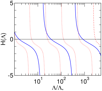
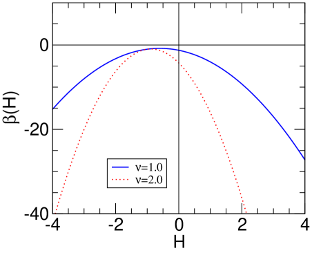
Figure 2: Left panel: The dimensionless coupling $H(\Lambda)$. Right panel: The $\beta$ function $\beta(H)$. The solid (dotted) line corresponds to $\nu=1$ ($\nu=2$).

In order to fix the relative phase $\alpha$ in Eq. (11), we can either specify both the cutoff $\Lambda$ and the dimensionless coupling $H$ or, using Eq. (14), one dimensionful parameter: $\Lambda_{*}$. This parameter $\Lambda_{*}$ is generated by the iteration of quantum corrections in solving the integral equation (13). In essence, this is the phenomenon of dimensional transmutation Wil99 .

In the left panel of Fig. 2, we show the functional dependence of $H$ on $\Lambda$ for $\nu=1$ (solid line) and $\nu=2$ (dashed line). It is evident that $H(\Lambda)$ runs on a limit cycle with a preferred scaling factor $\lambda_{0}=\exp(\pi/\nu)$. If the cutoff is increased or decreased by a factor $\lambda_{0}$, $H(\Lambda)$ returns to its original value. In contrast to the square-well regularization in configuration space Beane:2000wh , it is not possible to choose a continuous function for $H(\Lambda)$. The scale invariance of the bare potential is not compatible with the regulator. The renormalization breaks the full scale invariance of the $1/r^{2}$ potential (1) down to the discrete sub-group of scaling transformations with the preferred scaling factor $\lambda_{0}$. This is a simple example of a quantum-mechanical anomaly Braaten:2004pg .

Note also that $H(\Lambda)$ vanishes for a special set of cutoffs

$$\Lambda_{n}(\Lambda_{*})=\Lambda_{*}\exp(n\pi/\nu)\,,$$ (15)

where $n$ is an integer. We can therefore obtain a renormalized version of Eq. (13) that does not explicitly contain the counterterm by using the discrete set of cutoffs from Eq. (15). The same trick can be used for the three-body problem with large scattering length Hammer:2000nf .

Further insight can be gained by deriving the RG equation for $H$. Using the explicit solution (14), we find for the $\beta$ function by differentiating:

$$\Lambda\frac{d}{d\Lambda}H\equiv\beta(H)=-\frac{1}{4}(1-H)^{2}-\nu^{2}(1+H)^{2}\,.$$ (16)

This expression for $\beta(H)$ is shown in the right panel of Fig. 2 for the two cases $\nu=1$ (solid line) and $\nu=2$ (dotted line). Since $\beta(H)$ is negative definite for $\nu>0$, there are no fixed point solutions for $H$. The $\beta$ function has only two complex roots, $H_{\pm}=-(2\nu\pm i)/(2\nu\mp i)\,.$ It becomes maximal at $H_{max}=-(\nu^{2}-1/4)/(\nu^{2}+1/4)$ and takes the value $\beta(H_{max})=-\nu^{2}/(\nu^{2}+1/4)$. As $H$ approaches $\pm\infty$ the $\beta$ function approaches $-\infty$. In the limit $\nu\to 0$ ($\nu\to\infty$), the limit cycle disappears and a fixed point at $H=1$ ($H=-1$) emerges.

IV Observables

We now turn to the calculation of low-energy observables for the $1/r^{2}$ potential. We demonstrate explicitly that the scattering phases and the binding energies are independent of $\Lambda$ if $H(\Lambda)$ varies as given in Eq. (14). In particular, we discuss the manifestation of the limit cycle in the observables.

First, we consider the bound state spectrum. In Fig. 3, we show a part of the spectrum as

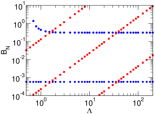
Figure 3: The bound state spectrum as a function of the cutoff for $H(\Lambda)\equiv 0$ (squares) and $H(\Lambda)$ given by Eq. (14) (circles).

a function of the cutoff $\Lambda$. The squares show the binding energies for the unrenormalized case: $H(\Lambda)\equiv 0$. The binding energies grow as the cutoff is increased and there is an accumulation point at threshold. The spectrum is bounded from below and the energy of the deepest state is of order $\Lambda^{2}$. However, if $H(\Lambda)$ varies according to Eq. (14), the binding energies are independent of $\Lambda$. The deepest state ist still of order $\Lambda^{2}$, but a new deeply-bound state appears whenever the cutoff is increased by a power of the preferred scaling factor $\lambda_{0}=\exp(\pi/\nu)$. The shallow binding energies, however, are not affected. In particular, the accumulation point at threshold persists since it is an infrared effect. This phenomenon is strongly related to the Efimov effect in the three-body problem with large scattering length where $\nu\approx 1.00624$ Efimov70 . As a consequence, all bound states within the range of the effective theory with binding energy $B\ll\Lambda^{2}$ are renormalized.

It is straightforward to show that if $B$ is a binding energy, then $\exp(2\pi/\nu)\,B$ is a solution as well. For dimensional reasons, the dependence of the binding energies on the cutoff is

$$\ln B_{N}=c_{1}-N\frac{2\pi}{\nu}+2\ln\Lambda\,,\qquad N\geq 0\,,\quad c_{1}=-2.07\pm 0.03\,,$$ (17)

where we have arbitrarily labelled the deepest state with $N=0$. The dependence of the renormalized energies on $\Lambda_{*}$ can be obtained by using Eq. (15).

We now turn to the scattering observables. From now on, we only consider the renormalized case. In Fig. 4, we show $\cot\delta(k)$ as a function of the center-of-mass momentum $k=\sqrt{E}$ for $\Lambda_{*}=1.0$ and two different values of $\nu$.

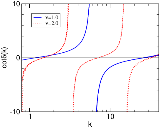
Figure 4: The quantity $\cot\delta$ as a function of $k$ for $\Lambda_{*}=1.0$ and $\nu=1$ (solid line) as well as $\nu=2$ (dotted line). Each curve corresponds to various calculations with cutoffs in the range $\Lambda=50\ldots 100$.

The solid line corresponds to $\nu=1$, while the dotted line corresponds to $\nu=2$. Each curve represents various calculations with cutoffs in the range $\Lambda=50\ldots 100$. The spread of the lines shows the cutoff dependence remaining after the counter term $\delta V$ is included. Note that the renormalization from the previous section is exact only at zero energy. For finite energy, there are corrections that are suppressed by powers of $k/\Lambda$. For momenta $k\ll\Lambda$, they are small and the phase shifts are practically independent of the cutoff $\Lambda$.

The discrete scaling symmetry requires that $\cot\delta(k)$ is a periodic function of $\nu\ln(k/\Lambda_{*})$. This is clearly statisfied in Fig. 4. It follows that the general form of the phase shifts in Fig. 4 can be written as

$$\delta(k)=\beta(\nu)-\nu\ln(k/\Lambda_{*})\,,$$ (18)

where $\beta$ is an angle that depends on $\nu$. From Eq. (18) and Fig. 4, it is evident that the phase shift is not defined in the limit $k\to 0$ FLS71 .

Another scattering observable that can be obtained from the phase shift is the total cross section for S-wave scattering

$$\sigma_{tot}=\int d\Omega|T(k)|^{2}=\frac{4\pi}{[k\cot\delta(k)]^{2}+k^{2}}\,.$$ (19)

In Fig. 5 we show $\sigma_{tot}$ as a function of $k=\sqrt{E}$

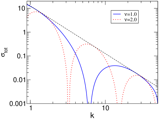
Figure 5: The total scattering cross section for $\Lambda_{*}=1.0$ and $\nu=1$ (solid line) as well as $\nu=2$ (dotted line). The dashed line indicates the unitarity limit $4\pi/k^{2}$.

for the same parameter values as in Fig. 4. The solid line corresponds to $\nu=1$, while the dotted line corresponds to $\nu=2$. The dashed line gives the unitarity limit $\sigma_{uni}=4\pi/k^{2}$. The total cross section saturates the unitarity limit exactly at those values of $k$ where $k\cot\delta(k)$ vanishes. It has zeros at the values of $k$ where $k\cot\delta(k)$ diverges. The dimensionless cross section $\sigma_{tot}/\sigma_{uni}$ is invariant under discrete scale transformations.

In summary, all low-energy observables display the discrete scaling symmetry. The limit cycle leads to log-periodic dependence of the observables on the counterterm parameter $\Lambda_{*}$. Furthermore, the limit cycle also becomes manifest in scattering observables via a log-periodic dependence on the energy. This is the case even if the counterterm strength can be chosen as a continuous function of the cutoff (cf. Ref. Beane:2000wh ).

V Summary & Conclusions

In this paper, we have studied the renormalization of the singular $1/r^{2}$ potential in momentum space. This potential is one of the simplest physical systems with a RG limit cycle. Interpreting this potential as an effective theory that breaks down at short distances, we have renormalized the corresponding Lippmann-Schwinger equation for S-waves by introducing a momentum cutoff $\Lambda$ and a momentum-independent counter term potential $\delta V\propto H(\Lambda)/\Lambda$.

Demanding invariance of low-energy observables under variations of the cutoff $\Lambda$, we have shown that the dimensionless function $H(\Lambda)$ runs on a limit cycle. The function $H(\Lambda)$ depends on a dimensionful parameter $\Lambda_{*}$ that must be specified in addition to the strength of the $1/r^{2}$ potential $\nu$ in order to characterize a physical system uniquely. Different values of $\Lambda_{*}$ correspond to physical systems with the same long range behavior but different short distance physics.

For our choice of regulator, a continuous dependence of the counterterm on $\Lambda$ is not possible. This is in contrast to renormalization of the $1/r^{2}$ potential with a square well potential in position space where a continuous dependence can be chosen Beane:2000wh .

The scale invariance of the bare $1/r^{2}$ potential is anomalous. It is not compatible with the regularization of the singularity of this potential at $r=0$. The scale invariance is broken down to the discrete subgroup of scaling transformations with the preferred scaling factor $\lambda_{0}=\exp(\pi/\nu)$ by the renormalization procedure.

The limit cycle of the counterterm potential becomes manifest in physical observables via the discrete scaling symmetry and the corresponding log-periodic behavior. While the periodic dependence of the counterterm potential on the cutoff $\Lambda$ appears to be dependent on the specific regulator, the discrete scaling symmetry is robust and regulator-independent. We have illustrated the manifestation of this scaling symmetry in the log-periodic behavior of low-energy observables on the energy by calculating the bound state spectrum, the S-wave scattering phase shifts, and the total S-wave cross section.

It will be interesting to see if the effect of limit cycles can be observed in experiment. The three-body physics of cold alkali atoms near a Feshbach resonance, where their interaction strength can be tuned by adjusting an external magnetic field, appears to be a promising avenue BrH04 . In Ref. Weber03 , the three-body recombination rate for ¹³³Cs atoms in the $|3,+3\rangle$ hyperfine state was measured in the interval 10 G $<B<$ 150 G which includes several Feshbach resonances. Unfortunately, the log-periodic behavior could neither be observed nor could it be excluded. Improved experiments are called for to resolve this question. Another indication of a limit cycle would be the observation of the Efimov effect. Recent experiments with Bose-Einstein condensates of ⁸⁵Rb atoms near a Feshbach resonance have produced evidence for a condensate of diatomic molecules coexisting with the atom condensate Don02 . It might be possible to create condensates of the triatomic molecules predicted by the Efimov effect coexisting with atom and dimer condensates Braaten:2002er . Finally, the attractive $1/r^{2}$ potential has been realized in experiment by neutral atoms interacting with a charged wire Dens98 .

- (1) S.R. Beane, P.F. Bedaque, L. Childress, A. Kryjevski, J. McGuire, and U. v. Kolck, Phys. Rev. A 64, 042103 (2001) [arXiv:quant-ph/0010073].
- (2) M. Bawin and S.A. Coon, Phys. Rev. A 67, 042712 (2003) [arXiv:quant-ph/0302199].
- (3) E. Braaten and D. Phillips, arXiv:hep-th/0403168.
- (4) T. Barford and M.C. Birse, J. Phys. A 38, 697 (2005) [arXiv:nucl-th/0406008].
- (5) K.G. Wilson, Rev. Mod. Phys. 55, 583 (1983).
- (6) D.J. Gross and F. Wilczek, Phys. Rev. Lett. 30, 1343 (1973).
- (7) H.D. Politzer, Phys. Rev. Lett. 30, 1346 (1973).
- (8) K.G. Wilson, Phys. Rev. D 3, 1818 (1971).
- (9) D. Sornette, Phys. Rep. 297, 239 (1998) [arXiv:cond-mat/9707012].
- (10) A.B. Zamolodchikov, JETP Lett. 43, 730 (1986) [Pisma Zh. Eksp. Teor. Fiz. 43, 565 (1986)].
- (11) A. Leclair, J.M. Roman, and G. Sierra, Nucl. Phys. B 675, 584 (2003) [arXiv:hep-th/0301042].
- (12) S. Albeverio, R. Hoegh-Krohn, and T.S. Wu, Phys. Lett. 83A, 105 (1981).
- (13) V. Efimov, Phys. Lett. 33B, 563 (1970).
- (14) V.N. Efimov, Sov. J. Nucl. Phys. 12, 589 (1971).
- (15) P.F. Bedaque, H.-W. Hammer, and U. van Kolck, Phys. Rev. Lett. 82, 463 (1999) [arXiv:nucl-th/9809025].
- (16) P.F. Bedaque, H.-W. Hammer, and U. van Kolck, Nucl. Phys. A 646, 444 (1999) [arXiv:nucl-th/9811046].
- (17) E. Braaten and H.-W. Hammer, arXiv:cond-mat/0410417.
- (18) E. Braaten and H.-W. Hammer, Phys. Rev. Lett. 91, 102002 (2003) [arXiv:nucl-th/0309030].
- (19) S.D. Glazek and K.G. Wilson, Phys. Rev. Lett. 89, 230401 (2002) [arXiv:hep-th/0203088].
- (20) S.D. Glazek and K.G. Wilson, Phys. Rev. B 69, 094304 (2004).
- (21) A. LeClair, J.M. Roman, and G. Sierra, Phys. Rev. B 69, 020505 (2004) [arXiv:cond-mat/0211338].
- (22) A. Anfossi, A. LeClair, and G. Sierra, arXiv:hep-th/0503014.
- (23) D. Bernard and A. LeClair, Phys. Lett. B 512, 78 (2001) [arXiv:hep-th/0103096].
- (24) A. LeClair, J.M. Roman, and G. Sierra, Nucl. Phys. B 700, 407 (2004) [arXiv:hep-th/0312141].
- (25) A. LeClair and G. Sierra, arXiv:hep-th/0403178.
- (26) K.M. Case, Phys. Rev. 80, 797 (1950).
- (27) W.M. Frank, D.J. Land, and R.M. Spector, Rev. Mod. Phys. 43, 36 (1971).
- (28) H.E. Camblong, L.N. Epele, H. Fanchiotti, and C.A. Garcia Canal, Phys. Rev. Lett. 85, 1590 (2000) .
- (29) E.J. Mueller and T.-L. Ho, arXiv:cond-mat/0403283.
- (30) D.B. Kaplan, arXiv:nucl-th/9506035;
- (31) G.P. Lepage, arXiv:nucl-th/9706029.
- (32) See, e.g., F. Wilczek, Nature 397, 303 (1999).
- (33) H.E. Camblong and C.R. Ordonez, Phys. Rev. D 68, 125013 (2003) [arXiv:hep-th/0303166].
- (34) H.-W. Hammer and T. Mehen, Nucl. Phys. A 690, 535 (2001) [arXiv:nucl-th/0011024].
- (35) T. Weber, J. Herbig, M. Mark, H.-C. Nägerl, and R. Grimm, Phys. Rev. Lett. 91, 123201 (2003).
- (36) E.A. Donley, N.R. Claussen, S.T. Thompson, and C.E. Wieman, Nature 417, 529 (2002) [arXiv:cond-mat/0204436].
- (37) E. Braaten, H.-W. Hammer, and M. Kusunoki, Phys. Rev. Lett. 90, 170402 (2003) [arXiv:cond-mat/0206232].
- (38) J. Denschlag, G. Umshaus, and J. Schmiedmayer, Phys. Rev. Lett. 81, 737 (1998).