Hamiltonian of Homonucleus Molecules for NMR Quantum Computing

Abstract

We derive the Hamiltonian in the rotating frame for NMR quantum computing with homonucleus molecules as its computational resource. The Hamiltonian thus obtained is different from conventional Hamiltonians that appear in literature. It is shown that control pulses designed for heteronucleus spins can be translated to pulses for homonucleus spins by simply replacing hard pulses by soft pulses with properly chosen pulse width. To demonstrate the validity of our Hamiltonian, we conduct several experiments employing cytosine as a homonucleus molecule. All the experimental results indicate that our Hamiltonian accurately describes the dynamics of the spins and that the conventional Hamiltonian fails. Finally we use our Hamiltonian for precise control of field inhomogeneity compensation with a pair of $\pi$-pulses.

I Introduction

Quantum computation currently attracts a lot of attention since it is expected to solve some of computationally hard problems for a conventional digital computer ref:1 . Numerous realizations of a quantum computer have been proposed to date. Among others, a liquid-state NMR (nuclear magnetic resonance) quantum computer is regarded as most successful. Early experiments demonstrated quantum teleportation nmr1 , quantum search algorithm nmr2 , quantum error correction nmr3 , and simulation of a quantum mechanical system nmr4 . Undoubtedly, demonstration of Shor’s factorization algorithm VSB01 is one of the most remarkable achievements in NMR quantum computation. Although the number of admissible qubits in a liquid-state NMR quantum computer is suspected to be limited up to about ten due to poor spin polarization at a room temperature, a liquid-state NMR quantum computer is one of few quantum computers that are capable of running nontrivial quantum algorithms thanks to well established NMR technology.

Since the number of qubits within heteronucleus spins is practically limited to two or three, the use of homonucleus spins is inevitable if we try to equip an NMR with a large number of qubits. It should be pointed out, however, that liquid-state NMR of homonucleus molecules is still poorly understood and literature dealing with this subject often lacks solid ground. Although the product operator formalism ernst has been extensively employed to implement quantum algorithms with an NMR quantum computer, people overlooked significance of the genuine Hamiltonian. Actually there is a subtle difference between the conventionally used Hamiltonian and the proper Hamiltonian for homonucleus spins. It is, therefore, urgently required to establish theoretical foundation underlying a liquid-state NMR quantum computer with homonucleus molecules.

Suppose we would like to implement a quantum algorithm whose unitary matrix representation is $U_{\rm alg}$. If the Hamiltonian $H$ depends on the control parameters, which we write collectively as $\gamma(t)$, the time evolution operator is given by

$$U[\gamma(t)]={\mathcal{T}}\exp\left[-i\int_{0}^{T}H(\gamma(t))dt\right],$$ (1)

where ${\mathcal{T}}$ stands for the time-ordering product. We use the natural unit in which $\hbar=1$. Optimal control of the quantum computer requires a control function $\gamma(t)$ that produces the specified quantum algorithm $U[\gamma(t)]=U_{\rm alg}$ in the shortest possible time $T$. Recently, numerical scheme to find the optimal control has been worked out for fictitious Josephson junction qubits, where polygonal paths in the parameter space has been utilized qaa4 ; qaa6 . For time-optimal control of an NMR quantum computer, another method employing the Cartan decomposition of SU($2^{n}$) has been proposed ref:kg and has been demonstrated experimentally with a two-qubit heteronucleus molecule qaa . We note that exact optimal control has been found for holonomic quantum computation in an idealized situation qaa3.5 .

This paper has three aims: (1) to provide the theoretical foundation for an NMR quantum computer with homonucleus molecules, (2) to show that any pulse sequence designed for heteronucleus molecules can be translated into that for homonucleus molecules, and (3) to demonstrate experimentally that our Hamiltonian accurately describes the dynamics of the spins. For these purposes, we carefully examine the Hamiltonians for NMR spin dynamics. Although the Hamiltonian for a homonucleus molecule is the same as the one for a heteronucleus molecule in the laboratory frame, the former looks quite different from the latter in a rotating frame.

This paper is organized as follows. In section II we study Hamiltonians of homonucleus as well as heteronucleus molecules. We carefully examine how they are transformed in a rotating frame and what is appropriate approximation to be employed. Surprisingly, our resulting Hamiltonian is different from the conventional Hamiltonian. In section III, we conduct several experiments to verify our analysis by taking cytosine as an example of homonucleus molecules. We execute the Deutsch-Jozsa algorithm, execute the pulse sequence for pseudo-pure state preparation, and verify the robustness of two-qubit entangling operations. As an application of the correct form of the Hamiltonian we implement field inhomogeneity compensation using a pair of $\pi$-pulses in section IV. Section V is devoted to conclusions and discussion.

II Hamiltonian in Rotating Frame

In this section, we write down the Hamiltonian of spin dynamics in the laboratory frame and transform it to the one in a rotating frame. Although the Hamiltonian for a homonucleus molecule has the same form as the one for a heteronucleus molecule in the laboratory frame, Hamiltonians in a rotating frame differ from each other.

We restrict ourselves within two-qubit molecules for simplicity. Generalization to molecules with more qubits is straightforward. As an example of heteronucleus molecules, we refer to ¹³C-labeled chloroform. The qubits are spins of ¹³C and H nuclei. We take cytosine solved in D₂O as an example of homonucleus molecule. The qubits are spins of two hydrogen nuclei (protons) in this case.

II.1 Heteronucleus molecule

II.1.1 Experimental setup

A liquid-state NMR consists of three parts as described in NMR_textbook . The first part is magnetic coils; a superconducting coil to generate a homogeneous static magnetic field and a normal conducting coil to generate temporally controlled field gradients. The second part contains resonance circuits for applying radio frequency (rf) magnetic fields to the sample. They are also used to pick up rf signals from the sample. The third part is an assembly of electronic circuits to feed rf pulses into the resonance circuits and to detect the signals picked up by the coils.

The NMR setup for heteronucleus molecules is shown schematically in Fig. 1. The first and second spins have respective resonance frequencies $\omega_{0,i}$ ($i=1,2$), which are also called Larmor frequencies. Their resonance frequencies are widely different for heteronucleus molecules under consideration. Hence two sets of resonance circuits and assembly of electronic circuits are required. The large difference of the resonance frequencies, $\Delta\omega_{0}=\omega_{0,2}-\omega_{0,1}$, allows us to address each spin individually with a short pulse.

Figure 1: NMR setup for heteronucleus molecules.

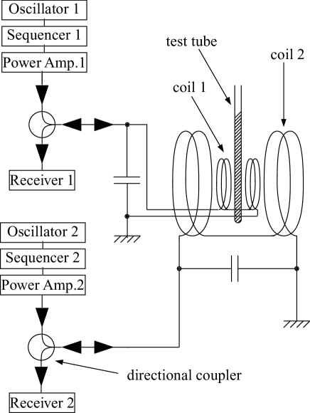
The oscillator $i$ $(i=1,2)$ in the third part generates an rf electric wave with frequency $\omega_{{\rm rf},i}$. The sequencer $i$ modulates the rf wave to shape a designed pulse. A typical temporal duration of a pulse, which is called the pulse width, is of the order of 10 $\mu$s. The rf pulses are amplified and fed into the resonance coil $i$, which generates rf magnetic fields applied to the sample in the test tube. Precession of spins in molecules appears as rotation of magnetization of the sample and induces a signal at the coil $i$. The receiver $i$ detects the signal. The directional coupler prevents transmission of the rf pulse from the amplifier to the receiver.

II.1.2 Heteronucleus molecule in rotating frame

The two-qubit Hamiltonian in the laboratory frame is

$$H=H_{0}+H_{{\rm rf},1}+H_{{\rm rf},2}.$$ (2)

Here the system Hamiltonian $H_{0}$ is defined as rmp_chuang

$$H_{0}=-\omega_{0,1}I_{z}\otimes I-\omega_{0,2}I\otimes I_{z}+\!\!\sum_{k=x,y,z}\!\!JI_{k}\otimes I_{k},$$ (3)

where $I_{k}=\sigma_{k}/2$, $\sigma_{k}$ being the $k$-th Pauli matrix, and $I$ is the unit matrix of dimension two. The first two terms in $H_{0}$ describe free precession of the spins in a static magnetic field while the third term describes the intramolecule spin interaction with coupling strength $J$.

$H_{{\rm rf},i}$ ($i=1,2$) represents the action of the rf magnetic field generated by the coil $i$ and hence is called the control Hamiltonian. Their explicit forms are

$$H_{{\rm rf},1}\!\! = \!\!-2\omega_{1,1}\cos(\omega_{{\rm rf},1}t-\phi_{1})(I_{x}\otimes I+gI\otimes I_{x}),$$ (4)

$$H_{{\rm rf},2}\!\! = \!\!-2\omega_{1,2}\cos(\omega_{{\rm rf},2}t-\phi_{2})(g^{-1}I_{x}\otimes I+I\otimes I_{x}).\;\;$$ (5)

Here, the amplitude of the rf pulse $\omega_{1,i}$, the frequency of the pulse $\omega_{{\rm rf},i}$ and the phase of the pulse $\phi_{i}$ are controllable parameters. We may assume, without loss of generality, that the rf field is applied along the $x$-axis in the laboratory frame. In the above equations we introduced the ratio of resonance frequencies of the two nuclei,

$$g=\frac{\omega_{0,2}}{\omega_{0,1}}.$$ (6)

We shall examine the transformation law of the Hamiltonians from the laboratory frame to a rotating frame. The spin dynamics in the laboratory frame is governed by the Liouville equation

$$i\frac{d\rho}{dt}=[H,\rho],$$ (7)

where $\rho$ is the density matrix of the system under consideration. The unitary operator

$$U=\exp(-i\omega_{{\rm rot},1}I_{z}t)\otimes\exp(-i\omega_{{\rm rot},2}I_{z}t)$$ (8)

transforms $\rho$ into the density matrix $\tilde{\rho}$ in the rotating frame as

$$\tilde{\rho}=U\rho\,U^{\dagger}.$$ (9)

Note that we can choose the rotation angular velocities $\omega_{{\rm rot},i}$ ($i=1,2$) arbitrarily. The time evolution of the system is now governed by

$$i\frac{d\tilde{\rho}}{dt}=[\tilde{H},\tilde{\rho}]$$ (10)

with the transformed Hamiltonian

$$\tilde{H} = UHU^{\dagger}-iU\frac{d}{dt}U^{\dagger}=\tilde{H}_{0}+\tilde{H}_{{\rm rf},1}+\tilde{H}_{{\rm rf},2}.$$ (11)

Here the transformed system Hamiltonian is

$$\tilde{H}_{0} = UH_{0}U^{\dagger}-iU\frac{d}{dt}U^{\dagger}$$ (16)

$$= -(\omega_{0,1}-\omega_{{\rm rot},1})I_{z}\otimes I$$

$$-(\omega_{0,2}-\omega_{{\rm rot},2})I\otimes I_{z}+JI_{z}\otimes I_{z}$$

$$+\left(\begin{array}[]{cccc}0&0&0&0\\ 0&0&\frac{J}{2}e^{i\Delta\omega_{\rm rot}t}&0\\ 0&\frac{J}{2}e^{-i\Delta\omega_{\rm rot}t}&0&0\\ 0&0&0&0\end{array}\right),$$

where $\Delta\omega_{\rm rot}\equiv\omega_{{\rm rot},2}-\omega_{{\rm rot},1}$. The transformed control Hamiltonians $\tilde{H}_{{\rm rf},i}$ will be given later. If we take the frame co-moving with each spin, which has the angular velocities $\omega_{{\rm rot},i}=\omega_{0,i}$, the first two terms in Eq. (16) vanish. In the case of heteronucleus molecules, the condition $\left|\Delta\omega_{0}\right|\gg J$ is always satisfied and thus the matrix elements in the last line also vanish after averaging over time. For example, $\left|\Delta\omega_{0}\right|/2\pi\sim 400$ MHz while $J/2\pi\sim 200$ Hz for ¹³C-labeled chloroform at 11 T, for which $\left|\Delta\omega_{0}\right|/J\sim 10^{6}$. Therefore $\tilde{H}_{0}$ is well approximated by

$$\tilde{H}_{0}=JI_{z}\otimes I_{z}.$$ (17)

When the resonance and co-rotating conditions $\omega_{{\rm rf},i}=\omega_{0,i}=\omega_{{\rm rot},i}$ are satisfied, the control Hamiltonians in the rotating frame

$$\tilde{H}_{{\rm rf},i}=UH_{{\rm rf},i}U^{\dagger}$$ (18)

are approximately given as

$$\tilde{H}_{{\rm rf},1} = -\omega_{1,1}(\cos\phi_{1}\,I_{x}\otimes I+\sin\phi_{1}\,I_{y}\otimes I),$$ (19)

$$\tilde{H}_{{\rm rf},2} = -\omega_{1,2}(\cos\phi_{2}\,I\otimes I_{x}+\sin\phi_{2}\,I\otimes I_{y})$$ (20)

after dropping terms rapidly oscillating with frequencies $2\omega_{0,i}$ and $\Delta\omega_{0}$. Note that the factor 2 in front of $\omega_{1,i}$ in Eqs. (4) and (5) has disappeared in Eqs. (19) and (20). This is physically understood as discussed in NMR_textbook ; a linearly polarized rf magnetic field oscillating with frequency $\omega_{\rm rf}$ is a superposition of two circularly polarized fields with frequencies $\pm\omega_{\rm rf}$ and the effect of the component with $-\omega_{\rm rf}$ is averaged to vanish. It is also important to notice that a pulse with frequency $\omega_{{\rm rf},i}$ influences only the spin $i$ and does not affect the other spin in the rotating frame. This is because $\left|\Delta\omega_{0}\right|$ is much larger than the inverse of the typical pulse width $\sim 1/(10\,\mu s)\sim 100$ kHz and hence the rf pulse resonating with one spin does not have spectral component which affects the other spin.

In conclusion, the Hamiltonian for a heteronucleus molecule in resonant magnetic fields is

$$\tilde{H} = JI_{z}\otimes I_{z}$$ (21)

$$-\omega_{1,1}(\cos\phi_{1}\,I_{x}\otimes I+\sin\phi_{1}\,I_{y}\otimes I)$$

$$-\omega_{1,2}(\cos\phi_{2}\,I\otimes I_{x}+\sin\phi_{2}\,I\otimes I_{y})$$

in the rotating frame that has the angular velocities $\omega_{{\rm rot},i}=\omega_{0,i}$.

II.2 Homonucleus molecules

II.2.1 Experimental setup

Figure 2: NMR setup for homonucleus molecules.

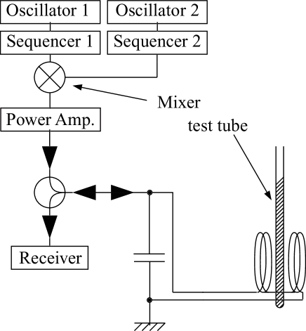
The NMR setup for homonucleus molecules is shown schematically in Fig. 2. Because the difference of the resonance frequencies $\Delta\omega_{0}=\omega_{0,2}-\omega_{0,1}$ is not large compared to $\omega_{0,i}$ in this case, a common resonance circuit and a power amplifier can be used to control both spins. For cytosine in D₂O, for example, we find $\left|\Delta\omega_{0}\right|/2\pi\sim 765.0$ Hz while $\omega_{0,i}/2\pi\sim 500$ MHz. Although the difference $\Delta\omega_{0}$ is small, it still allows us to address respective spins individually provided that the pulse width is sufficiently long.

The oscillator $i$ generates a continuous rf electric wave with frequency $\omega_{{\rm rf},i}=\omega_{0,i}$. The sequencer shapes the continuous wave into pulses. When addressing the two spins simultaneously, a typical pulse width is of the order of 10 $\mu$s. On the other hand, when addressing them individually, a typical pulse width is of the order of $2\pi/\left|\Delta\omega_{0}\right|\sim 1$ ms. The rf pulses from the two sequencers are mixed and amplified. The coil generates magnetic fields and picks up signals from the sample and the receiver detects the signals. Due to close resonance frequencies $\omega_{0,i}$, only one set of resonance circuit and receiver is necessary for homonucleus molecules.

II.2.2 Homonucleus molecule in rotating frame

The Hamiltonian for homonucleus molecule in the laboratory frame has the identical form to the Hamiltonian for a heteronucleus molecule (2). Even for homonucleus molecule the condition $\left|\Delta\omega_{0}\right|\gg J$ is satisfied in general. For example, in the case of cytosine in D₂O, $\left|\Delta\omega_{0}\right|/2\pi\sim 765.0$ Hz while $J/2\pi\sim 7.1$ Hz, and thus the above condition is satisfied. Therefore, the approximation used in the derivation of the system Hamiltonian (17) for a heteronucleus molecule is also applicable to derivation of that for a homonucleus molecule. Thus the system Hamiltonian of a homonucleus molecule takes the form

$$\tilde{H}_{0}=JI_{z}\otimes I_{z}.$$ (22)

in the co-rotating frame of each spin.

The control Hamiltonian $\tilde{H}_{{\rm rf},i}$ describes the action of the resonant magnetic field in the frame rotating with angular velocity $\omega_{{\rm rot},i}=\omega_{0,i}=\omega_{{\rm rf},i}$. Corresponding Hamiltonian $\tilde{H}_{{\rm rf},i}$ for homonucleus molecule is considerably more complicated even when terms rapidly oscillating with frequencies $2\omega_{0,i}$ and $\omega_{0,1}+\omega_{0,2}$ are averaged out as

$$\tilde{H}_{{\rm rf},1} = -\omega_{1,1}\Big{[}\cos\phi_{1}\,I_{x}\otimes I+\sin\phi_{1}\,I_{y}\otimes I$$ (23)

$$+g\cos(\Delta\omega_{0}t+\phi_{1})I\otimes I_{x}$$

$$+g\sin(\Delta\omega_{0}t+\phi_{1})I\otimes I_{y}\Big{]},$$

$$\tilde{H}_{{\rm rf},2} = -\omega_{1,2}\Big{[}\cos\phi_{2}\,I\otimes I_{x}+\sin\phi_{2}\,I\otimes I_{y})$$ (24)

$$+g^{-1}\cos(-\Delta\omega_{0}t+\phi_{2})I_{x}\otimes I$$

$$+g^{-1}\sin(-\Delta\omega_{0}t+\phi_{2})I_{y}\otimes I\Big{]}.$$

If we further assume that the pulse width $\tau$ are long enough so that even slowly oscillating terms in Eqs. (23) and (24), which contain $\Delta\omega_{0}$, are averaged out, then Eqs. (23) and (24) reduce to Eqs. (19) and (20). Simultaneously, we can tune the pulse width $\tau$ short enough ($J\tau\ll 1$) so that the spin-spin interaction (22) is negligible while pulses are applied. Therefore we conclude that an arbitrary pulse sequence designed for heteronucleus molecules works for homonucleus ones provided that all the hard pulses are replaced by soft pulses whose pulse width $\tau$ satisfies the condition $2\pi/\left|\Delta\omega_{0}\right|<\tau\ll 2\pi/J$. We will demonstrate this consequence experimentally in the next section, where we set $\tau=4(2\pi/\left|\Delta\omega_{0}\right|)=5.229$ ms $\ll 2\pi/J=140.8$ ms.

II.3 Conventional Hamiltonians

Here we make comparison between the Hamiltonians derived in the previous subsection and the Hamiltonian for homonucleus molecules used in literature. Conventionally the system Hamiltonian

$$\tilde{H}_{{\rm conv},0}=-\Delta\omega_{0}I\otimes I_{z}+JI_{z}\otimes I_{z}$$ (25)

is used to describe spin dynamics in a static magnetic field in a rotating frame cory2 . Apparently, it differs from our Hamiltonians (22).

We suspect that the Hamiltonian (25) may be derived from the original system Hamiltonian (3) via transformation from the laboratory frame to the frame rotating with a common angular velocity $\omega_{{\rm rot},1}=\omega_{{\rm rot},2}=\omega_{0,1}$. We will show, however, that this choice does not yield the Hamiltonian (25) in the rotating frame.

If we take a frame that rotates with a common angular velocity equal to $\omega_{0,1}$ for both spins, transformation operator (8) becomes

$$U_{\rm com}=\exp(-i\omega_{0,1}I_{z}t)\otimes\exp(-i\omega_{0,1}I_{z}t).$$ (26)

Then the system Hamiltonian (3) is transformed into

$$\tilde{H}_{{\rm com},0} = U_{\rm com}H_{0}U_{\rm com}^{\dagger}-iU_{\rm com}\frac{d}{dt}U_{\rm com}^{\dagger}$$ (31)

$$= -\Delta\omega_{0}I\otimes I_{z}+JI_{z}\otimes I_{z}$$

$$+\left(\begin{array}[]{cccc}0&0&0&0\\ 0&0&\frac{J}{2}&0\\ 0&\frac{J}{2}&0&0\\ 0&0&0&0\end{array}\right),$$

which does not agree with the conventional Hamiltonian (25).

Another system Hamiltonian in the laboratory frame

$$H_{{\rm conv},0}=-\omega_{0,1}I_{z}\otimes I-\omega_{0,2}I\otimes I_{z}+JI_{z}\otimes I_{z}$$ (32)

is also sometimes employed in literature rmp_chuang ; cory ; raedt but this is also different from the original system Hamiltonian (3). We cannot take the Hamiltonian (32) as a correct one since we cannot replace $\sum_{k}JI_{k}\otimes I_{k}$ by $JI_{z}\otimes I_{z}$ in the laboratory frame.

To illustrate the difference between our Hamiltonian and the conventional Hamiltonian, let us consider the unitary gate

$$U_{\rm E} = \exp(-i\pi I_{z}\otimes I_{z})$$ (37)

$$= \left(\begin{array}[]{cccc}e^{-i\pi/4}&0&0&0\\ 0&e^{i\pi/4}&0&0\\ 0&0&e^{i\pi/4}&0\\ 0&0&0&e^{-i\pi/4}\end{array}\right),$$

which is employed along with one-qubit operations to implement the controlled-NOT gate ref:1 . We implement the gate $U_{\rm E}$ from our system Hamiltonian (22), as

$$U_{J}(\pi/J)=\exp(-i\pi\tilde{H}_{0}/J)=\exp(-i\pi I_{z}\otimes I_{z}).$$ (38)

In other words, we simply wait for a time interval $T_{J}=\pi/J$ without applying any rf pulses. Let us define the distance between $U_{\rm E}$ and $U_{J}(t)$ as

$$\|U_{\rm E}-U_{J}(t)\|\equiv\sqrt{{\rm tr}[(U_{\rm E}-U_{J}(t))^{\dagger}(U_{\rm E}-U_{J}(t))]}.$$ (39)

This is easily evaluated as

$$\|U_{\rm E}-U_{J}(t)\|=2\sqrt{2}\sqrt{1-\cos\frac{1}{4}(Jt-\pi)}.$$ (40)

We observe that the distance vanishes at $t=T_{J}$ so that $U_{J}(T_{J})=U_{\rm E}$. We note also that the distance remains close to zero in the vicinity $t\sim T_{J}$. This robust character of $U_{J}(t)$ was clearly observed in our experiment as shown in the next section.

On the other hand, if we replace $\tilde{H}_{0}$ in Eq. (38) by the conventional Hamiltonian (25), the distance between $U_{\rm E}$ and $U_{J}(t)$ becomes

$$\|U_{\rm E}-U_{{\rm conv}J}(t)\|$$ (41)

$$= 2\sqrt{2}\sqrt{1-\cos\Big{(}\frac{\Delta\omega_{0}t}{2}\Big{)}\cos\frac{1}{4}(Jt-\pi)}.$$

Therefore, if the conventional Hamiltonian (25) were a correct one to describe the spin dynamics, $U_{{\rm conv}J}(t)$ would not coincide with $U_{\rm E}$ at $t=T_{J}$ and the distance $\|U_{\rm E}-U_{{\rm conv}J}(t)\|$ should oscillate in the vicinity of the $t\sim T_{J}$. However, such a rapid oscillation in time has not been observed in our experiment.

III Experiments

III.1 Spectrometer and molecules

All the data were taken at room temperature with a JEOL ECA-500 spectrometer jeol , where the hydrogen Larmor frequency is approximately 500 MHz.

We used 0.6 mL, 23 mM sample of cytosine cytosine solved in D₂O. The measured coupling strength is $J/2\pi=7.1$ Hz while the frequency difference is $\left|\Delta\omega_{0}\right|/2\pi=765.0$ Hz. The transverse relaxation time $T_{2}$ is measured to be $\sim 1$ s for both hydrogen nuclei and the longitudinal relaxation time $T_{1}$ is $\sim 7$ s.

In order to measure the spin states, we apply a reading pulse to only one spin, called spin 1, and then obtained the spectrum by Fourier transforming the free induction decay (FID) signal. The state of the spin 1 is read from the sign of the peak in the spectrum while the state of the other nucleus (spin 2) is found from the peak position.

III.2 Deutsch-Jozsa algorithm

The Deutsch-Jozsa (DJ) algorithm DJ is one of the simplest quantum algorithms that illustrate the power of quantum computation and has been implemented by several groups 13c ; cytosine . Let us consider a one-bit function $f:\{0,1\}\to\{0,1\}$. For a two-qubit register, there are only four possibilities for $f$, whose explicit forms are $f_{1}(0)=f_{1}(1)=0$, $f_{2}(0)=f_{2}(1)=1$, $f_{3}(0)=0,f_{3}(1)=1$ and $f_{4}(0)=1,f_{4}(1)=0$. The former two functions are said to be “constant” while the latter two are “balanced”. With the DJ algorithm, we can tell whether a given unknown function $f$ is constant or balanced via only a single trial.

Chuang et al. 13c employed carbon-13 labeled chloroform, a heteronucleus molecule, as a computational resource while Jones and Mosca cytosine used cytosine, a homonucleus molecule, to execute the DJ algorithm. Chuang et al. executed the DJ algorithm using the pulse sequences shown in Table 1. According to our previous discussions, it should be possible to use the pulse sequences of Chuang et al. for cytosine molecules by simply replacing hard pulses with soft ones.

The results of our quantum computations with cytosine are summarized in Figs. 3 and 4. We started the computation with the thermal equilibrium state since the DJ algorithm does not require a pure initial state 13c .

Table 1: Control pulse sequences for the Deutsch-Jozsa algorithm taken from the reference 13c . The functions $f_{i}(x)$ are defined in the text. Here, $[\frac{\pi}{2}]_{i}$ denotes the $\pi/2$ pulses around the $i$-axes $(i=x,y,-x,-y)$. The symbol $[\pi]$ denotes the $\pi$ pulse around the $x$-axis. (1/$nJ$) denotes the two-qubit entangling operation produced by turning off the rf pulses during the interval $2\pi/nJ$. The pulse sequences are followed by a readout $\pi/2$ pulse around the $x$-axis to the spin 1, which is not shown in the Table. The receiver detects the FID (free induction decay) signal to measure the spin state.

Gate	Pulse sequence
$f_{1}$
spin 1	$[\frac{\pi}{2}]_{y}$	–	(1/4$J$)	–	(1/4$J$)	–	$[\frac{\pi}{2}]_{-y}$
spin 2	$[\frac{\pi}{2}]_{-y}$	–	(1/4$J$)	$[\pi]$	(1/4$J$)	$[\pi]$	$[\frac{\pi}{2}]_{y}$
$f_{2}$
spin 1	$[\frac{\pi}{2}]_{y}$	–	(1/4$J$)	–	(1/4$J$)	–	$[\frac{\pi}{2}]_{-y}$
spin 2	$[\frac{\pi}{2}]_{-y}$	–	(1/4$J$)	$[\pi]$	(1/4$J$)	–	$[\frac{\pi}{2}]_{y}$
$f_{3}$
spin 1	$[\frac{\pi}{2}]_{y}$	–	(1/2$J$)	$[\frac{\pi}{2}]_{-y}$	$[\frac{\pi}{2}]_{-x}$	$[\frac{\pi}{2}]_{y}$	$[\frac{\pi}{2}]_{-y}$
spin 2	$[\frac{\pi}{2}]_{-y}$	$[\frac{\pi}{2}]_{y}$	(1/2$J$)	$[\frac{\pi}{2}]_{-y}$	$[\frac{\pi}{2}]_{x}$	–	$[\frac{\pi}{2}]_{y}$
$f_{4}$
spin 1	$[\frac{\pi}{2}]_{y}$	–	(1/2$J$)	$[\frac{\pi}{2}]_{-y}$	$[\frac{\pi}{2}]_{-x}$	$[\frac{\pi}{2}]_{y}$	$[\frac{\pi}{2}]_{-y}$
spin 2	$[\frac{\pi}{2}]_{-y}$	$[\frac{\pi}{2}]_{y}$	(1/2$J$)	$[\frac{\pi}{2}]_{-y}$	$[\frac{\pi}{2}]_{-x}$	–	$[\frac{\pi}{2}]_{y}$

Figure 3: The FID spectra of the spin 1 in cytosine showing output of the DJ algorithms. The sign of each peak indicates the state of the spin 1. The location of each peak indicates the state of the spin 2. When the initial state of the spin 2 is $|0\rangle$, it causes a larger shift to the resonance frequency of the spin 1 and contributes to a left peak in each curve. Then the sign of the left peak discriminates whether $f_{i}$ is constant or balanced. The left peak is positive for $f_{1}$ and $f_{2}$ (constant) and negative for $f_{3}$ and $f_{4}$ (balanced). The numbers in the left side are durations of the two-qubit operations in ms. The correct duration of the two-qubit operations is $T_{J}=70.4$ ms. Note that the spectra are insensitive to variation of the two-qubit operation time.

III.2.1 $J$-coupling time

The DJ algorithm employs the $J$-coupling unitary operator $U_{J}(t)$ with $t=2\pi/4J=T_{J}/2$ or $t=2\pi/2J=T_{J}$ to entangle two spins. The time durations for the two-qubit operations are $2\pi/4J+2\pi/4J=T_{J}$ for $f_{1}$ and $f_{2}$ and $T_{J}$ for $f_{3}$ and $f_{4}$. Thus the total execution time is $T_{J}$ for all four cases.

As we discussed when we derived Eq. (40), our Hamiltonian (22) predicts that $U_{J}(t)$ does not deviate much from the desired unitary transformation even when the gate operation time $t$ deviates from the correct value. On the other hand, Eq. (41) tells us that the conventional Hamiltonian (25) predicts that $U_{J}(t)$ sharply depends on the timing $t$ and oscillates as $\cos(\Delta\omega_{0}t/2)$.

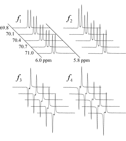
In experiment we executed the DJ algorithm with various gate operation time $t$ in the vicinity of $T_{J}$ and observed how the resulting spectra depend on $t$. We employed the pulse sequences shown in Table 1, in which all hard pulses used by Chuang et al. 13c were replaced with Gaussian soft pulses with the pulse width 5.229 ms.

The initial state of the molecules is a thermal mixture of four states $|00\rangle$, $|01\rangle$, $|10\rangle$, and $|11\rangle$. The DJ algorithm does not work when the second qubit is $|1\rangle$ and fails to distinguish constant from balanced. On the other hand, it works regardless of the state of the first qubit. In Fig. 3 the peaks with a smaller frequency shift (the right peaks) are outputs from the initial states $|01\rangle$ or $|11\rangle$. In this case the algorithm fails to distinguish if $f_{i}$ is constant or balanced. The peaks with a larger frequency shift (the left peaks) in Fig. 3 are outputs from the initial states $|00\rangle$ or $|10\rangle$. In this case the DJ algorithm successfully tells us if $f_{i}$ is constant or balanced by the sign of the peak (positive for $f_{1}$ and $f_{2}$ while negative for $f_{3}$ and $f_{4}$).

We varied the $J$-coupling time interval $t$ in the range from 69.8 ms to 71.0 ms. In other words, $\Delta\omega_{0}t/2$ was swept between $26.7\times 2\pi$ and $27.2\times 2\pi$. The exact duration to produce the designed unitary operator correctly is 70.4 ms. We observe from Fig. 3 that the spectra are not sensitive to variation of the time interval. Therefore we concluded that our Hamiltonian (22) accounts for the experimental results consistently.

III.2.2 Rf pulse width

In literature cytosine ; raedt it is recommended to use soft pulses whose width is an integral multiple of $2\pi/\left|\Delta\omega_{0}\right|$ in order to avoid undesirable effect caused by the term $\Delta\omega_{0}I\otimes I_{z}$ in the conventional Hamiltonian (25). Our discussion and experiment show that this tuning is not necessary since the relevant Hamiltonian (22) does not contain the term $\Delta\omega_{0}I\otimes I_{z}$.

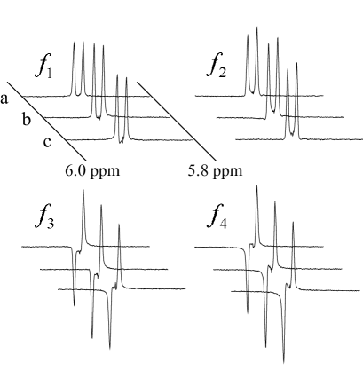
We executed the DJ algorithms shown in Table 1, with different pulse width (5.229 and 6.217 ms). In our setting, the pulse width 5.229 ms is equal to $4\times 2\pi/\left|\Delta\omega_{0}\right|$, while 6.217 ms is $4.76\times 2\pi/\left|\Delta\omega_{0}\right|$. The measured FID spectra of the spin 1 are shown in Fig. 4. No significant changes in the spectra appeared even if we tuned the pulse width to a fractional multiple of $2\pi/\left|\Delta\omega_{0}\right|$. This result proves that the pulse width need not be an integral multiple of $2\pi/\left|\Delta\omega_{0}\right|$ to implement a given gate and obtain a reasonable spectrum.

Figure 4: The effect of variation of the pulse widths on the spectrum of the DJ algorithms. The pulse widths for spins 1 and 2 are (a) 5.229 ms and 5.229 ms, (b) 6.217 ms and 6.217 ms, and (c) 5.229 ms and 6.217 ms, respectively. Observe that the spectra are insensitive to the variation of pulse width.

IV Field Inhomogeneity Compensation

Here we discuss an experiment to reveal the nature of the Hamiltonians (23) and (24), which depict the action of the oscillating magnetic fields on the spins. It is common to employ the compensating pulse method to suppress errors induced by field inhomogeneity. We will show, by employing our Hamiltonian, that the entangling operation with the $J$-coupling is fragile in the presence of the compensating pulses and a fine tuning of the gate operation time is required.

IV.1 $\pi$-pulse pair in J-coupling time

We have shown in the previous section that it is not necessary to tune the $J$-coupling time very accurately since this operation is robust against small change of the gate operation time. However, if the system is under the influence of field inhomogeneity, it may cause an error during the $J$-coupling time.

It is well known that this undesired effect caused by field inhomogeneity can be compensated by a series of hard $\pi$-pulse pair, whose width is of the order of 10 $\mu$s. The best known example may be the CPMG (Carr-Purcell-Meiboom-Gill) pulse sequence NMR_textbook . Let us apply this technique to $U_{J}(t)$. Then the pulse sequence for $U_{J}(t)$ is replaced with

$$U_{J*}(t)\,:\,U_{J}(t/2)-[\pi]-U_{J}(t/2)-[\pi],$$ (42)

where time flows from left to right and $[\pi]$ denotes a hard pulse that rotates both spins by $\pi$ radian. We take the rotation axis to be the $x$-axis of one of the spins, for example the spin 1, while the rotation axis for the other spin, the spin 2, depends on the time when the $[\pi]$ is applied, according to the Hamiltonian (23). The pulse sequence is represented as the product of unitary matrices

$$U_{J*}(t)=U_{1,\pi}^{(2)}\,U_{J}(t/2)\,U_{1,\pi}^{(1)}\,U_{J}(t/2),$$ (43)

where

$$U_{1,\pi}^{(1)} = \exp(-i\pi I_{x}\otimes I)$$

$$\times \exp(-i\pi[\cos(\Delta\omega_{0}\frac{t}{2})I\otimes I_{x}+\sin(\Delta\omega_{0}\frac{t}{2})I\otimes I_{y}]),$$

$$U_{1,\pi}^{(2)} = \exp(-i\pi I_{x}\otimes I)$$

$$\times \exp\left(-i\pi[\cos(\Delta\omega_{0}t)I\otimes I_{x}+\sin(\Delta\omega_{0}t)I\otimes I_{y}]\right).$$

Note that we put the ratio of resonance frequencies $g=\omega_{0,2}/\omega_{0,1}=1$ for the homonucleus molecule. The resulting operator $U_{J*}(t)$ does not coincides with $U_{J}(t)$. The distance between $U_{J*}(t)$ and $U_{\rm E}$ is evaluated as

$$\|U_{\rm E}-U_{J*}(t)\|$$ (46)

$$= 2\sqrt{2}\sqrt{1-\cos\Big{(}\frac{\Delta\omega_{0}t}{2}\Big{)}\cos\frac{1}{4}(Jt-\pi)}.$$

The distance does not vanish generally because the two conditions, $\cos(\Delta\omega_{0}t/2)=\pm 1$ and $\cos(Jt/4-\pi/4)=\pm 1$, are rarely satisfied simultaneously. Moreover, the distance is very sensitive to $t$.

Table 2: Control pulse sequences to create the pseudo-pure state $|00\rangle$ pps_j . Here, $[\frac{\pi}{m}]_{i}$ denotes the $\frac{\pi}{m}$ pulse around the $i$-axes $(i=x,y,-x,-y)$ while (1/2$J$) denotes the two-qubit entangling operation implemented by turning off the rf pulses during the interval $2\pi/2J$. The symbol FG denotes application of a pulsed field gradient for spatial labeling. The pulse sequence is followed by a readout $\pi/2$-pulse around the $x$-axis to the spin 1, which is not shown in the Table.

	Pulse sequence
spin 1		FG	$[\frac{\pi}{4}]_{x}$	(1/2$J$)	$[\frac{\pi}{4}]_{-y}$	FG
spin 2	$[\frac{\pi}{3}]_{x}$	FG		(1/2$J$)		FG

IV.2 Pseudo-pure state preparation

Figure 5: The effect of variation of the $J$-coupling time on the spectrum of the pseudo-pure state creation. The spectra in the left panel are measured without the $\pi$-pulse pair in the entangling operation. The spectra in the right panel are measured with the $\pi$-pulse pair. The numbers are the two-qubit operation time in ms. Note that the spectra generated with the $\pi$-pulse pair are sensitive to variation of the two-qubit operation time.

An NMR quantum computer must be initialized to the pseudo-pure state $|00\rangle$ before executing a specific algorithm. This initialization procedure is implemented with the pulse sequence pps_j shown in Table 2. In this section we examine the effect of the compensating $\pi$ pulses on the initialization procedure.

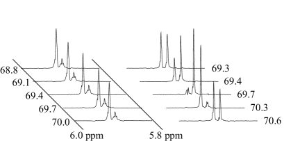
The initialization process contains the $J$-coupling time, in which the two spins are entangled by the two-qubit operation $U_{J}(t)$. We vary the gate operation time $t$ to introduce an operational error on purpose. It is possible, however, to apply a pair of $\pi$-pulses to compensate this error while the $J$-coupling is under action as instructed in Eq. (42). We have swept the gate operation time between 69.3 ms and 70.6 ms and the results are summarized in Fig. 5.

The spectra in the left panel of Fig. 5 were measured without applying the $\pi$-pulse pair in the entangling operation. We observed that the spectra are robust against small variations of the gate operation time. The intense peaks with a larger frequency shift are signals from molecules in the $|00\rangle$ state while the smaller peaks are error signals from small amount of molecules not in the $|00\rangle$ state.

The spectra in the right panel were measured with the $\pi$-pulse pair applied during the entangling operation. We observed that the spectra are very sensitive to the variation of the $J$-coupling operation time, although it is still possible to adjust the operation time so that the desired pseudo-pure state is produced with a good precision. When the gate operation time was set at the correct value $t=70.3$ ms, the spectrum exhibited a sharper peak than those in the left panel. This result implies that the $\pi$-pulse pair improved the quality of the initialized state. However, the spectra were fragile when the duration $t$ deviates from the correct value. For example, when the duration was set at $t=69.7$ ms, the intense signal indicated that the most of molecules are in the $|01\rangle$ state, and not in the desired state $|00\rangle$.

Thus we conclude that our Hamiltonian (23) and (24) accurately account for the experimental results.

V Conclusions and Discussion

We have derived the relevant Hamiltonian for homonucleus molecules in NMR quantum computing and shown that any pulse sequence for a heteronucleus molecule may be translated into that for a homonucleus molecule by simply replacing hard pulses by soft pulses with a properly chosen pulse width. We have demonstrated that the NMR spectra in several experiments are accounted for with our Hamiltonian but not with the conventional Hamiltonian found in literature. It was shown in our experiments that the spectra are robust under small variations of the $J$-coupling operation time as well as of the rf pulse widths. Moreover, we provided the theoretical basis for field inhomogeneity compensation by a pair of hard $\pi$ pulses during the entangling operation and verified it experimentally.

Generalization of the present work to molecules with more spins is straightforward. It is easy to find proper pulse sequence, either numerically qaa or by Cartan decomposition ref:kg ; warp , once an exact form of the Hamiltonian is obtained. Theoretical analysis as well as experiments on these subjects are under progress and will be published elsewhere.

References

- (1) M. A. Nielsen and I. L. Chuang, Quantum Computation and Quantum Information (Cambridge University Press, Cambridge, 2000).
- (2) M. A. Nielsen, E. Knill, and R. Laflamme, Nature 396 52 (1998).
- (3) I. L. Chuang, N. Gershenfeld, and M. Kubinec, Phys. Rev. Lett. 80 3408 (1998).
- (4) D. G. Cory, M. D. Price, W. Maas, E. Knill, R. Laflamme, W. H. Zurek, T. F. Havel, and S. S. Somaroo. Phys. Rev. Lett. 81 2152 (1998).
- (5) S. Somaroo, C. H. Tseng, T. F. Havel, R. Laflamme, and D. G. Cory, Phys. Rev. Lett. 82 5381 (1999).
- (6) L. M. K. Vandersypen, M. Steffen, G. Breyta, C. S. Yannonl, M. H. Sherwood, and I. L. Chuang, Nature 393 143 (1998).
- (7) R. R. Ernst, G. Bodenhausen, and A. Wokaun, Principles of Nuclear Magnetic Resonance in One and Two Dimensions (Oxford University Press, Oxford, 1991).
- (8) A. O. Niskanen, J. J. Vartiainen, and M. M. Salomaa, Phys. Rev. Lett. 90, 197901 (2003).
- (9) J. J. Vartiainen, A. O. Niskanen, M. Nakahara, and M. M. Salomaa, Phys. Rev. A 70, 012319 (2004).
- (10) N. Khaneja, R. Brockett, and S. J. Glaser, Phys. Rev. A 63, 032308 (2001).
- (11) M. Nakahara, Y. Kondo, K. Hata, and S. Tanimura, Phys. Rev. A 70, 052319 (2004).
- (12) S. Tanimura, M. Nakahara, and D. Hayashi, J. Math. Phys. 46, 022101 (2005).
- (13) For example, see T. E. W. Claridge, High-Resolution NMR techniques in Organic Chemistry (Elsevier, Amsterdam, 2004).
- (14) L. M. K. Vandersypen and I. L. Chuang, Rev. Mod. Phys. 76, 1037 (2004).
- (15) R. lamme, E. Knill, D. G. Cory, E. M. Fortunato, T. F. Havel, C. Miquel, R. Martinez, C. J. Negrevergne, G. Ortiz, M. A. Pravia, Y. Sharf, S. Sinha, R. Somma, and L. Viola, Los Alamos Science Number 27, 226 (2002).
- (16) D. G. Cory, R. Laflamme, E. Knill, L. Viola, T. F. Havel, N. Boulant, G. Boutis, E. Fortunato, S. Lloyd, R. Martinez, C. Negrevergne, M. Pravia, Y. Sharf, G. Teklemariam, Y. S. Weinstein, and W. H. Zurek, Fortschr. Phys. 40, 875 (2000), J. A. Jones, Fortschr. Phys. 40, 909 (2000).
- (17) H. De Raedt, K. Michielsen, A. Hams, S. Miyashita, and K. Saito, Eur. Phys. J. B 27, 15 (2002).
- (18) http://www.jeol.com/nmr/nmr.html.
- (19) J. A. Jones, M. Mosca, and R. H. Hansen, J. Chem. Phys. 109 1648 (1998).
- (20) D. Deutsch, Proc. R. Soc. Lond. A 400, 97 (1985), D. Deutsch and R. Jozsa, Proc. R. Soc. Lond. A 439, 533 (1985).
- (21) I. L. Chuang, L. M. K. Vandersypen, X. Zhou, D. W. Leung, and S. Lloyd, Nature 393, 143 (1998).
- (22) U. Sakaguchi, H. Ozawa, and T. Fukumi, Phys. Rev. A 61, 042313 (2000).
- (23) M. Nakahara, J. J. Vartiainen, Y. Kondo, S. Tanimura, and K. Hata, e-print quant-ph/0411153.