Experimental implementation of local adiabatic evolution algorithms by an NMR quantum information processor

Abstract

Quantum adiabatic algorithm is a method of solving computational problems by evolving the ground state of a slowly varying Hamiltonian. The technique uses evolution of the ground state of a slowly varying Hamiltonian to reach the required output state. In some cases, such as the adiabatic versions of Grover’s search algorithm and Deutsch-Jozsa algorithm, applying the global adiabatic evolution yields a complexity similar to their classical algorithms. However, using the local adiabatic evolution, the algorithms given by J. Roland and N. J. Cerf for Grover’s search [ Phys. Rev. A. 65 042308(2002)] and by Saurya Das, Randy Kobes and Gabor Kunstatter for the Deutsch-Jozsa algorithm [Phys. Rev. A. 65, 062301 (2002)], yield a complexity of order $\sqrt{N}$ (where N=2ⁿ and n is the number of qubits). In this paper we report the experimental implementation of these local adiabatic evolution algorithms on a two qubit quantum information processor, by Nuclear Magnetic Resonance.

I 1. Introduction

Quantum algorithms provide elegant opportunities to harness available quantum resources and perform certain computational tasks more efficiently than classical devices. The idea that a quantum computer could simulate the physical behavior of a quantum system as well as perform computation, attracted immediate attention preskill ; ss . The theory of such quantum computers is now well understood and several quantum algorithms like Deutsch-Jozsa (DJ) algorithm deu , Grover’s search algorithm grover , Shor’s prime factorization algorithm shor , Hogg’s algorithm hogg ,Bernstein-Vazirani problem vazi and quantum counting count1 have been developed . All these algorithms start from a well-defined initial state and perform computation by a sequence of reversible logic gates. After computation, the final state of the system gives the output. Various methods are being examined for building a quantum information processing (QIP) device which is coherent and unitary bou . Nuclear Magnetic Resonance has emerged as a leading candidate for implementation of various quantum computational problems on a small number of qubits cory97 ; chuang97 ; cory98 ; djchu ; djjo ; grochu ; grojo ; ka1 ; ka ; jcp ; nat ; ranapra2 ; ijqi ; ranapra1 ; ranabirtomo .

Quantum adiabatic algorithms provide an alternative method for computing ad1 ; ad2 . In this method the computation is done by evolving the system under a Hamiltonian for a given amount of time. Such algorithms start from a suitable input ground state and by evolution under a slowly time-varying Hamiltonian, reach the desired output state. Quantum adiabatic algorithms have been efficiently applied to solve various optimization problems ad3 ; ad4 ; ad5 ; ad6 . Chuang et al. have demonstrated the implementation of a quantum adiabatic algorithm by solving the MAX-CUT garey problem on a three qubit system by NMR chu . In these algorithms, the condition for adiabaticity is fulfilled globally by using only the minimum energy gap between the ground state and the first excited state for calculating the time of evolution. This method of evolution is not efficient in some cases such as adiabatic Grover’s search algorithm and adiabatic Deutsch-Jozsa algorithm as they result in a complexity O(N) (N is the size of the data set), which is as good as their classical algorithms. However, these algorithms can be improved by application of local adiabatic evolution, where the adiabatic condition is fulfilled at each instant of time. This technique has been adopted theoretically by Roland and Cerf cerf for the adiabatic Grover’s search algorithm and by S. Das et al. for adiabatic Deutsch-Jozsa algorithm das yielding a complexity O($\sqrt{N}$). Experimental implementation of adiabatic Grover’s search algorithm based on the proposal of Roland and Cerf and adiabatic Deutsch-Jozsa algorithm of S. Das et al., is reported here. Section 2 contains an introduction to adiabatic algorithms. Section 3 discusses the adiabatic version of the Grover’s search algorithm proposed by Roland and Cerf and its NMR implementation. Section 4 discusses the adiabatic Deutsch-Jozsa algorithm and its NMR implementation. Section 5 contains the experimental results, on a 2-qubit system, for both these algorithms. To the best of our knowledge this is the first experimental implementation of adiabatic Grover’s search and adiabatic Deutsch-Jozsa algorithms.

II 2. Adiabatic Algorithm

The adiabatic theorem of quantum mechanics states that when a system is evolved under a slowly time varying Hamiltonian, it stays in its instantaneous ground state me . This fact is used in solving certain computational problems ad3 ; ad4 ; ad5 ; ad6 . The problem to be solved is encoded in a final Hamiltonian ($H_{F}$), whose ground state is not easy to find. Adiabatic algorithms start with the ground state of a beginning Hamiltonian ($H_{B}$) which is easy to construct and whose ground state is also easy to prepare. The ground state of $H_{B}$, which is a superposition of all the eigenstates of H_F, is evolved under a time varying Hamiltonian $H(s)$. $H(s)$ is a linear interpolation of the beginning Hamiltonian $H_{B}$ and the final Hamiltonian $H_{F}$ such that

$$H(s)=(1-s)H_{B}+sH_{F},\hskip 85.35826pt\mbox{where}\;\;\;0\leq s\leq 1.$$ (1)

The parameter $s=t/T_{total}$, where $T_{total}$ is the total time of evolution and $t$ varies from 0 to $T_{total}$. After evolution under the Hamiltonian $H(s)$ for a time $T_{total}$, the system is in the ground state of $H_{F}$ with a probability $(1-\varepsilon^{2})^{2}$, provided the evolution rate satisfies,

$$\frac{\underset{0\leq s\leq 1}{max}\left|\left<1;s\left|\frac{dH(s)}{dt}\right|0;s\right>\right|}{g_{min}^{2}}\leq\varepsilon,$$ (2)

and the parameters of the algorithm are chosen to make $\varepsilon\ll$1 ad1 . The numerator in Eq. 2 is the transition amplitude between the ground state and the first excited state of H(s), and the denominator is the square of the smallest energy gap $(g_{min})$ between them. Ideally the time of evolution ($T_{total}$) must be infinite. However as long as the gap is finite, for any finite and positive $\varepsilon$, the time of evolution can be finite. The time of evolution of the algorithm is determined by the minimum energy gap between the ground state and the first excited state. In the adiabatic case the time of evolution determines the complexity of the algorithms (that is how long it takes for the task to be completed), which can then be compared to the complexity of the discrete algorithms in classical and quantum paradigms. The time of evolution is measured in units of natural time scale associated with the system, $\bar{T}$ which is O($\hbar/{\bar{E}}$) where $\bar{E}$ is the fundamental energy scale associated with the physical system used to construct the states. das .

In the actual implementation, the Hamiltonian $H(s)$ is discretized into $M+1$ steps as $H(\frac{m}{M})$ where m goes from $0\rightarrow M$ chu ; wvd . Thus the time varying Hamiltonian $H(s)$ goes from beginning Hamiltonian to final Hamiltonian in M+1 steps. As the total number of steps increase, the evolution becomes more and more adiabatic chu . The evolution operator for the m^th step is given by chu

$$U_{m}=e^{-i[(1-\frac{m}{M})H_{B}+\frac{m}{M}H_{F}]\Delta t},$$ (3)

where $\Delta t=T/(M+1)$. The total evolution is given by,

$$U=\prod_{m=0}^{M}U_{m}.$$ (4)

Since, $H_{B}$ and $H_{F}$ do not commute in general, the evolution operator of Eq. 3 is approximated to first order in $\Delta$t, by the use of the Trotter’s formula chu as

$$U_{m}\approx e^{-iH_{B}(1-\frac{m}{M})\frac{\Delta t}{2}}\cdot e^{-iH_{F}\frac{m}{M}\Delta t}\cdot e^{-iH_{B}(1-\frac{m}{M})\frac{\Delta t}{2}}.$$ (5)

Thus in each step only a small evolution of the system from ground state of ${\rm H_{B}}$ towards the ground state of ${\rm H_{F}}$ takes place.

III 3. Grover’s search algorithm

Suppose we are given an unsorted database of N items and one of those items is marked. To search for the marked item classically, it would require on an average N/2 queries. However using quantum resources, the algorithm prescribed by Grover grover performs the same search with O($\sqrt{N}$) queries. The algorithm starts with an equal superposition of states, representing the items, repeatedly flips the amplitude of the marked state (done by the oracle) followed by the flip of the amplitudes of all the states about the mean. The number of times this process is repeated determines the complexity of the algorithm and this scales with the size of the database as O($\sqrt{N}$).
In the adiabatic version, the system is evolved under a time dependent Hamiltonian which is a linear interpolation of H_B and H_F. As n qubits are used to label a database of size N (=2ⁿ), the resulting Hilbert space is of dimension N. The basis states in this space are $|i\rangle$ where i=0,$\cdots$,N. H_B is chosen such that the ground state is a linear superposition of all the basis states. Therefore for a 2-qubit case,

$$|\psi_{B}\rangle = \frac{1}{2}\left(|00\rangle+|01\rangle+|10\rangle+|11\rangle\right).$$ (6)

$$H_{B} = I-|\psi_{B}\rangle\langle\psi_{B}|,$$ (7)

$$= I-\frac{1}{4}\begin{pmatrix}1&1&1&1\cr 1&1&1&1\cr 1&1&1&1\cr 1&1&1&1\end{pmatrix}.$$ (8)

The Final Hamiltonian has the marked state $|\psi_{F}\rangle$ as the ground state.

$$H_{F} = I-|\psi_{F}\rangle\langle\psi_{F}|.$$ (9)

The rate at which the interpolating Hamiltonian H(s) (given by Eq. 1) changes from $H_{B}$ to $H_{F}$ depends on the condition,

$$\left|\frac{ds}{dt}\right|\leq\varepsilon\frac{g^{2}(s)}{\left|\langle\frac{dH}{ds}\rangle\right|}.$$ (10)

Following Roland and Cerf cerf , t is obtained as a function of s as,

$$t=\frac{1}{2\varepsilon}\frac{N}{\sqrt{N-1}}\left[arctan\{\sqrt{N-1}\left(2s-1\right)\}+arctan\sqrt{N-1}\right].$$ (11)

Taking t${}^{\prime}=\varepsilon t$ and on inverting the above function, s(t^′) is obtained as

$$s(t^{\prime})=\frac{1}{2}\left[\{\frac{1}{\sqrt{N-1}}tan\left(\frac{2\sqrt{N-1}t^{\prime}}{N}-arctan\sqrt{N-1}\right)\}+1\right].$$ (12)

The plot of this function for N=4 (for a 2 qubit case) is given in Fig. 1. In the experiment the time of evolution is varied according to Eq. 12. It has been shown by Roland and Cerf cerf that with this adiabatic evolution, the complexity of the algorithm is O($\sqrt{N}$).

IV 3.1. Experimental Implementation

The NMR Hamiltonian for a weakly coupled two-spin system is :

$${\mathcal{H}}=-\omega_{1}I_{z1}-\omega_{2}I_{z2}+2\pi J_{12}I_{z1}I_{z2}.$$ (13)

where $\omega_{1}$ and $\omega_{2}$ are Larmour frequencies and $J_{12}$ the indirect spin-spin coupling. The beginning Hamiltonian for a 2-qubit Grover’s algorithm as stated in Eq. 8, written in terms of spin-half operators, is

$${\mathcal{H}}_{B}=\frac{3}{4}I-\frac{1}{2}\{I_{x1}+I_{x2}+2I_{x1}I_{x2}\}.$$ (14)

The identity term does not cause any evolution of the state and so it can be omitted, yielding the beginning Hamiltonian without the negative sign and the factor half as:

$$\tilde{\mathcal{H}}_{B}=I_{x1}+I_{x1}+2I_{x1}I_{x2}$$ (15)

The evolution under $\tilde{\mathcal{H}}_{B}$ can be simulated by a free evolution under the Hamiltonian ${\mathcal{H}}$ of Eq. 13 between two $\pi$/2 pulses with appropriate phases.

$$e^{i\frac{\pi}{2}\left(I_{y1}+I_{y2}\right)}\cdot e^{i{\mathcal{H}}T}\cdot e^{-i\frac{\pi}{2}\left(I_{y1}+I_{y2}\right)} = e^{i\left(\omega_{1}I_{x1}+\omega_{2}I_{x2}+2JI_{x1}I_{x2}\right)T}$$ (16)

$$= e^{i{\mathcal{H}}^{\prime}T}$$ (17)

Let the state $|00\rangle$ be the marked state. The final Hamiltonian is,

$$H_{F}^{|00\rangle}=I-\begin{pmatrix}1&0&0&0\cr 0&0&0&0\cr 0&0&0&0\cr 0&0&0&0\cr\end{pmatrix}$$ (18)

In terms of spin operators the final Hamiltonian is,

$${\mathcal{H}}_{F}^{|00\rangle}=\frac{3}{4}I-\frac{1}{2}\left[I_{z1}+I_{z2}+2I_{z1}I_{z2}\right]$$ (19)

The final Hamiltonian keeping the spin operator terms only and without the negative sign and the factor half is

$$\tilde{\mathcal{H}}_{F}^{|00\rangle}=I_{z1}+I_{z2}+2I_{z1}I_{z2}$$ (20)

Similarly the final Hamiltonian for other states being marked, in terms of the spin-half operators, is

$$\tilde{\mathcal{H}}_{F}^{|01\rangle} = I_{z1}-I_{z2}-2I_{z1}I_{z2}$$ (21)

$$\tilde{\mathcal{H}}_{F}^{|10\rangle} = -I_{z1}+I_{z2}-2I_{z1}I_{z2}$$ (22)

$$\tilde{\mathcal{H}}_{F}^{|11\rangle} = -I_{z1}-I_{z2}+2I_{z1}I_{z2}$$ (23)

The schematic representation of the experiment for the adiabatic Grover’s algorithm in a two qubit system [consisting of a ¹H spin and a ¹³C spin] is shown in Fig. 2a. The experiment is divided into three parts. The first part (preparation part) consists of preparation of pseudo-pure state (PPS) followed by equal superposition. The second part is the adiabatic evolution, and the third part is the tomography of the resultant state. The pulse programme for the preparation of PPS and equal superposition is shown in Fig. 2b. The PPS is prepared by the method of spatial averaging du . After preparing PPS, equal superposition of states is obtained by application of the Hadamard gate on both the qubits. The Hadamard gate is implemented by $(\pi/2)_{y}$ -pulses, followed by $\pi_{x}$ -pulses on both proton and carbon spins (Fig. 2b) grochu . The next stage consists of adiabatic evolution which has been carried out in the present work in 60 steps. Each step of the adiabatic evolution (Figs. 2c, 2d, 2e and 2f) consists of evolution under the final Hamiltonian for a time $\tau$ sandwiched between two evolutions under the beginning Hamiltonian for a time (T-$\tau$)/2. T is the total evolution time for one step and is equal to 1/$\pi$J. The value of $\tau(=s\times\frac{1}{\pi J})$ varies from 0 to T takes place as ‘s’ increases from 0 to 1 according to Eq. 12, in 60 steps. The pulse sequence for the beginning Hamiltonian is a free evolution of the system juxtaposed between two $\pi$/2 pulses with appropriate phases on each of the spins (the part marked as H_B in Figs. 2c-2f). The pulse sequence for the final Hamiltonian depends on the marked state as stated in Eqs. 21-23. If the state $|00\rangle$ is the marked state, then the pulse sequence for the implementation of the final Hamiltonian is a free evolution of the system under the NMR Hamiltonian juxtaposed between two $\pi$ pulses on each of the spins (Fig. 2c). Similarly, if the state $|01\rangle$ is marked the pulse sequence for the final Hamiltonian is a free evolution of the system between two $\pi$ pulses on the spin 1 (Fig. 2d), if the state $|10\rangle$ is marked then the pulse sequence is a free evolution between two $\pi$ pulses on the spin 2 (Fig. 2e) and if the state $|11\rangle$ is marked, then the pulse sequence simulating the final Hamiltonian is just a free evolution of the system under the NMR Hamiltonian (Fig. 2f).

The third stage of the experiment is the tomography of the final density matrix after the adiabatic evolution. The density matrix of a 2-spin system is a 4$\times$4 matrix consisting of 6 independent off-diagonal complex elements (the remaining 6 are their complex conjugates), and the four diagonal elements which are the populations of the various levels. The diagonal elements are measured by 90^o pulses on each qubit preceded by a gradient pulse. The six off-diagonal elements consist of four single quantum (SQ), one double quantum (DQ) and one zero quantum (ZQ) coherences. The real and the imaginary SQ, DQ and ZQ coherences in terms of the spin operators are;

$${\rm SQ}^{real}_{i} = I_{ix}\pm 2(I_{ix}I_{jz}),$$ (24)

$${\rm SQ}^{imag}_{i} = I_{iy}\pm 2(I_{iy}I_{jz}),$$ (25)

$${\rm DQ}^{real} = 2(I_{ix}I_{jx}-I_{iy}I_{jy}),$$ (26)

$${\rm DQ}^{imag} = 2(I_{iy}I_{jx}+I_{ix}I_{jy}),$$ (27)

$${\rm ZQ}^{real} = 2(I_{ix}I_{jx}+I_{iy}I_{jy}),$$ (28)

$${\rm ZQ}^{imag} = 2(I_{iy}I_{jx}-I_{ix}I_{jy}),$$ (29)

where i$\neq$ j = 1,2 represents the qubits. Although the single quantum terms are directly observable, for proper scaling, all the off-diagonal elements are observed by a common protocol of two experiments;

$${\rm A:}\hskip 85.35826pt\left(\frac{\pi}{2}\right)^{i}_{\phi_{1}}\left(\theta\right)^{j}_{\phi_{2}}\longrightarrow G_{z} \longrightarrow\left(\frac{\pi}{2}\right)^{i}_{y},$$ (30)

$${\rm B:}\hskip 85.35826pt\left(\frac{\pi}{2}\right)^{i}_{\phi_{1}}\left(\theta\right)^{j}_{\phi_{2}}\longrightarrow G_{z} \longrightarrow\left(\pi\right)^{j}\left(\frac{\pi}{2}\right)^{i}_{y}.$$ (31)

where $\theta$ denotes the pulse angle, $\phi_{1}$, $\phi_{2}$ the pulse phases and $G_{z}$ a gradient pulse. The first two pulses of the experiment A (depending on the pulse angle $\theta$ and the pulse phases $\phi_{1}$ and $\phi_{2}$) convert terms like $I_{i\alpha}+2I_{i\alpha}I_{j\beta}$ into diagonal terms given by $I_{iz}+2I_{iz}I_{jz}$, where $\alpha$ and $\beta$ denote the x, y, or z component of the spin operators of the first and the second qubit respectively. The gradient destroys all the transverse magnetization retaining only the longitudinal terms. The last pulse converts the retained longitudinal magnetization $I_{iz}+2I_{iz}I_{jz}$ into observable terms $I_{ix}+2I_{ix}I_{jz}$. Thus the magnitude of $I_{i\alpha}+2I_{i\alpha}I_{j\beta}$ is mapped on to $I_{ix}+2I_{ix}I_{jz}$ which is then observed. In experiment B, a $\pi$-pulse is applied on the spin ‘j’ just before the $\pi$/2 pulse on the spin ‘i’. This creates the observable term $I_{ix}-2I_{ix}I_{jz}$. The sum and difference of the two experiments yields 2$I_{i\alpha}$ and 2$I_{i\alpha}I_{j\beta}$ respectively. Six different experiments are needed to be performed to map the whole density matrix (real and imaginary). The various pulse angles and phases required during the experiment, and the resultant terms that are observed due to them are given in Table I. Experiments I and II yield the SQ, and experiments III-VI yield the ZQ and DQ coherences.

V 4. Deutsch-Jozsa Algorithm

The Deutsch-Jozsa Algorithm determines whether a binary function $f(x)$,

$$f(x|x\in\{0,1\}^{n})\rightarrow\{0,1\},$$

is Constant or Balanced dja .A constant function implies that the function has the same value 0 or 1 for all $x$. A balanced function implies that the function ‘f’ is 0 for half the values of $x$ and 1 for the other half . For a two qubit case the constant and the balanced functions are given in Table II.

In the adiabatic version of the Deutsch-Jozsa algorithm, the beginning Hamiltonian and its ground state, for a two qubit system, is given by Eq. 8 and Eq. 6 respectively. The final Hamiltonian is given by Eq. 9 and the ground state of the final Hamiltonian for two qubits is of the form das ;

$$|\psi_{F}\rangle = \alpha|00\rangle+\frac{\beta}{\sqrt{3}}\left(|01\rangle+|10\rangle+|11\rangle\right),$$ (32)

where

$$\alpha = \frac{1}{4}\left|(-1)^{f(00)}+(-1)^{f(01)}+(-1)^{f(10)}+(-1)^{f(11)}\right|,$$ (33)

$$\beta^{2} = 1-\alpha^{2}.$$ (34)

From Eq. 34 it is seen that when $\alpha=1$ the function $f$ is constant, and when $\alpha=0$ then it is balanced. Thus $\alpha$ is chosen depending on whether the function to be encoded in the final Hamiltonian is constant or balanced. Using Eqs. 1,8,9,32 and 34 the matrix for the interpolating Hamiltonian($H(s)$) can be written as das ;

$$H(s)=I-\frac{1-s}{4}\begin{pmatrix}1&1&1&1\\ 1&1&1&1\\ 1&1&1&1\\ 1&1&1&1\end{pmatrix}-\frac{s}{3}\begin{pmatrix}3\alpha&0&0&0\\ 0&\beta&\beta&\beta\\ 0&\beta&\beta&\beta\\ 0&\beta&\beta&\beta\end{pmatrix}.$$ (35)

S. Das et al.  have shown that on evolution under the Hamiltonian $H(s)$ takes the initial state $|\psi_{B}\rangle$ to the solution state $|\psi_{F}\rangle$ das . In the next section we describe an NMR implementation of the above algorithm.

VI 4.1. NMR Implementation

The adiabatic Deutsch-Jozsa algorithm also, is implemented on the 2-qubit system. The beginning Hamiltonian in terms of the spin-half operators is the same as given in Eq. 15, and its implementation has been discussed in section 3.1.
The final Hamiltonian, obtained from Eqs. 8, 9, 32 and 34, for constant case ($\alpha$=1) yields,

$$H_{F}^{c}=I-\begin{pmatrix}1&0&0&0\cr 0&0&0&0\cr 0&0&0&0\cr 0&0&0&0\end{pmatrix},$$ (36)

and for balanced case ($$\alpha$$=0) yields,

$$H_{F}^{b}=I-\frac{1}{3}\begin{pmatrix}0&0&0&0\cr 0&1&1&1\cr 0&1&1&1\cr 0&1&1&1\end{pmatrix}.$$ (37)

The above final Hamiltonians in terms of spin-half operators can be written respectively as,

$${\mathcal{H}}_{F}^{c}=\frac{3}{4}I-\frac{1}{2} (I_{z1}+I_{z2}+2I_{z1}I_{z2}),$$ (38)

and,

$${\mathcal{H}}_{F}^{b}=\frac{3}{4}I-\frac{1}{3} \biggl{[}-\frac{1}{2}(I_{z1}+I_{z2}+2I_{z1}I_{z2})+2(I_{x1}I_{x2}+I_{y1}I_{y2})$$ (39)

$$+I_{x1}+I_{x2}-2(I_{x1}I_{z2}+I_{z1}I_{x2})\biggr{]}.$$ (40)

As the identity does not cause any evolution of the state we consider only the spin operator terms. Thus the final Hamiltonian keeping only the spin operators (dropping the minus sign), for the constant case, can be written as

$$\tilde{{\mathcal{H}}}^{c}_{F} = \frac{1}{2}\{I_{z1}+I_{z2}+2I_{z1}I_{z2}\},$$ (41)

and for the balanced case as

$$\tilde{{\mathcal{H}}}^{b}_{F}=-\frac{1}{6}(I_{z1} +I_{z2}+2I_{z1}I_{z2})+\frac{2}{3}(I_{x1}I_{x2}+I_{y1}I_{y2})$$ (42)

$$+\frac{1}{3}I_{x1}+\frac{1}{3}I_{x2}-\frac{2}{3}(I_{x1}I_{z2}+I_{z1}I_{x2}).$$ (43)

The signs of Eqs. 15, 41 and 43 are changed for consistency. Since the various terms in Eq. 43 do not commute, the evolution under this Hamiltonian would require a complex pulse sequence in NMR. However, we have found that by keeping only the diagonal terms in the Eq. 43, the pulse sequence simplifies considerably with the information regarding the balanced nature of the problem still encoded in it. This truncated final Hamiltonian for the balanced case is given by;

$$(\tilde{\mathcal{H}}^{b}_{F})^{trunc}=-\frac{1}{6}(I_{z1}+I_{z2}+2I_{z1}I_{z2})$$ (44)

The opposite signs of Eq. 41 and Eq. 44 distinguish the constant and the balanced case. In the following we show that the balanced nature of the Deutsch-Jozsa problem is still encoded in $(\tilde{\mathcal{H}}_{F}^{b})^{trunc}$. Substituting $\alpha=0$ and $\beta=1$ and dropping the off-diagonal terms from the last part of Eq. 35 , we obtain

$$\tilde{H}^{b}(s)=I-\frac{1-s}{4}\begin{pmatrix}1&1&1&1\\ 1&1&1&1\\ 1&1&1&1\\ 1&1&1&1\end{pmatrix}-\frac{s}{3}\begin{pmatrix}0&0&0&0\\ 0&1&0&0\\ 0&0&1&0\\ 0&0&0&1\end{pmatrix}.$$ (45)

The eigenvalues of this Hamiltonian are:

$$\lambda_{0} = \frac{1}{6}\left[3+2s-\sqrt{9+s(7s-15)}\right],$$ (46)

$$\lambda_{1} = \frac{1}{6}\left[3+2s+\sqrt{9+s(7s-15)}\right],$$ (47)

$$\lambda_{2} = \lambda_{3}=1-\frac{s}{3}.$$ (48)

The values of $\lambda_{0}$, $\lambda_{1}$, $\lambda_{2}$ and $\lambda_{3}$ as a function of ‘s’ are plotted in Fig. 3. $\lambda_{0}$ is the ground state. As ‘s’ increases from 0, $\lambda_{0}$ continues to be the ground state and becomes the ground state of the final Hamiltonian in the limit $s\rightarrow 1$. The eigenvectors corresponding to $\lambda_{0}$, $\lambda_{1}$, $\lambda_{2}$ and $\lambda_{3}$ are respectively obtained as;

$$v_{0}\!=\!\begin{pmatrix}\frac{3-s-2\sqrt{9-15s+7s^{2}}}{3(s-1)}\cr 1\cr 1\cr 1\end{pmatrix},\;v_{1}\!=\!\begin{pmatrix}\frac{3-s+2\sqrt{9-15s+7s^{2}}}{3(s-1)}\cr 1\cr 1\cr 1\end{pmatrix},\;v_{2}\!=\!\begin{pmatrix}0\cr-1\cr 0\cr 1\end{pmatrix},\;v_{3}\!=\!\begin{pmatrix}0\cr-1\cr 1\cr 0\end{pmatrix},$$ (49)

The final state to which the system converges after the evolution is

$$\underset{s\rightarrow 1}{lim}\;v_{0}=\begin{pmatrix}0\cr 1\cr 1\cr 1\end{pmatrix},$$ (50)

which is the desired output state.

The energy gap between the ground state and the states corresponding to $\lambda_{2}$ and $\lambda_{3}$ goes to zero as $s\rightarrow 1$ as shown in Fig. 3. However, there is no transition from $\lambda_{0}$ to $\lambda_{2}$, $\lambda_{3}$ as the transition amplitude given by the numerator in Eq. 2 is zero in these cases. Therefore the transition amplitude from the ground state $\lambda_{0}$ to the next excited state $\lambda_{1}$ is relevant for calculation of $s(t)$. The minimum energy gap between $\lambda_{0}$ and $\lambda_{1}$, needed in Eq. 2, is obtained for $s\simeq 1$ as seen in Fig. 3. Since the algorithm is implemented using local adiabatic evolutions we need to change $s(t)$ such that the adiabatic condition cerf

$$\frac{ds}{dt}\leq\varepsilon\frac{\left|g(s)\right|^{2}}{\left|\left<\frac{dH}{ds}\right>\right|},$$ (51)

is met at each time interval. Here g(s) is the energy gap between the ground state and the first excited state, given by $\frac{1}{3}\sqrt{9-15s+7s^{2}}$ and $\left|\left<dH/ds\right>\right|=H_{F}-H_{B}$. The Hamiltonian is evolved at a rate that is a solution of

$$\frac{ds}{dt}=\varepsilon\frac{\left|g(s)\right|^{2}}{\left|H_{F}-H_{B}\right|}$$ (52)

On integrating Eq. 52, we obtain t as a function of s.

$$t=\frac{1}{\varepsilon}\frac{14s-15}{2\sqrt{3}\sqrt{7s^{2}-15s+9}}+k,$$ (53)

where the constant of integration $k=\frac{5}{\varepsilon 2\sqrt{3}}$ to obey $s=0$ at $t=0$. Inverting this function we obtain $s(t^{\prime})$ as

$$s(t^{\prime})=\frac{3}{14}\left[5-\frac{\sqrt{225+24t\left(55\sqrt{3}-183t+60\sqrt{3}t^{2}-18t^{3}\right)}}{3+20\sqrt{3}t-12t^{2}}\right]$$ (54)

where $t^{\prime}$ is $\varepsilon t$. The plot of $s$ as a function of $t^{\prime}$ is shown in Fig. 4. From Figs. 3 and 4 it is seen that the rate of change of $s$ (and hence of the Hamiltonian) is fast when the energy gap between $\lambda_{0}$ and $\lambda_{1}$ is large, and slow when the gap is small. In practice the time of evolution for $H_{B}$ and $H_{F}$ is given by $(1-s)\times T$ and $s\times T$ respectively, where $T$ is 1/$\pi$J and $s$ is varied from 0 to 1 according to Eq. 53. In our implementation, the $t^{{}^{\prime}}$ interval for which $s$ varies from 0 to 1 is divided in 80 equal steps, and the corresponding values of s for each step (calculated from Eq. 48) are substituted in the evolution time of $H_{B}$ and $H_{F}$.
On integrating Eq. 46 from s=0 to s=1, we get the total time of evolution

$$T_{total}=\frac{1}{\varepsilon}\frac{2}{\sqrt{3}}{\bar{T}}.$$ (55)

T_total is given in the units of ${\bar{T}}$ which is the time scale associated with the physical system used das . The time scale associated with evolution under the NMR Hamiltonian is $\sim 10^{-3}s$. The total time of evolution of the experiment ($T_{total}$) is given by 80$\times$T, where T is the time for one step (see Fig. 5b). For the choice $\varepsilon\sim 10^{-2}$, T $\sim 60\times 10^{-3}$s in our case.

VII 4.2. Experimental Implementation

The experimental implementation of adiabatic Deutsch-Jozsa algorithm on a 2-qubit system [consisting of a ¹H spin and a ¹³C spin] also consists of three parts namely preparation, adiabatic evolution and tomography of the final density matrix. The preparation of the pseudo pure state (PPS) and making of equal superposing of states as well as the tomography of the final states has already been discussed in section 3. So we only describe the method of implementation of the final Hamiltonian for the Deutsch-Jozsa algorithm.
The pulse sequence for the implementation of the constant case final Hamiltonian ($\tilde{\mathcal{H}}_{F}^{c}$) is given in Fig. 5b. The beginning Hamiltonian is implemented by a free evolution juxtaposed between $\pi$/2 pulses with required phases (Fig. 5b). The implementation of the final Hamiltonian for the constant case is a free evolution under the NMR Hamiltonian of Eq. 14, juxtaposed between two $\pi$-pulses as shown in Fig. 5b. In the balanced case the implementation of the beginning Hamiltonian is same as in Fig. 5b. However, the implementation of the final Hamiltonian $(\tilde{\mathcal{H}}_{F}^{b})^{trunc}$ is done in two parts [Fig. 5c]. The first part is a free evolution under the Hamiltonian given in Eq. 14 [${\rm T_{f}}$ period in Fig. 5c]. The operator corresponding to such an evolution for time $\tau$ will be of the form;

$$e^{i\pi J(-I_{z1}-I_{z2}+2I_{z1}I_{z2})\tau}.$$ (56)

In the second evolution of $2\tau$, the chemical shifts are refocused so that the system evolves only under its scalar coupling Hamiltonian $2\pi JI_{z1}I_{z2}$. Just before and after the evolution $\pi$-pulses with appropriate phases are put on each of the spins to flip the sign of the corresponding spin operator [${\rm T_{j}}$ period in Fig. 5c]. The operator for the sequence of two pulses with an intermediate evolution for $2\tau$ is of the form

$$e^{-i(I_{x1})\pi}\cdot e^{i\pi J(2I_{z1}I_{z2})2\tau}\cdot e^{i(I_{x1})\pi}=e^{-i\pi J(2I_{z1}I_{z2})2\tau}.$$ (57)

As these two evolutions given in Eq. 56 and Eq. 57 commute, the effective evolution for the 3$\tau$ period is:

$$e^{i\pi J(-I_{z1}-I_{z2}+2I_{z1}I_{z2})\tau}\cdot e^{-i\pi J(2I_{z1}I_{z2})2\tau}=e^{i\pi J(-I_{z1}-I_{z2}-2I_{z1}I_{z2})\tau}.$$ (58)

Thus the evolution during ${\rm T_{j}}$ cancels the J-evolution during ${\rm T_{f}}$ and adds a minus sign to it, yielding the effective Hamiltonian of Eq. 58 and an effective evolution time of $\tau$. An evolution time of $\tau$=1/$\pi$J implements the full Hamiltonian of Eq. 39 as required for adiabatic evolution. Overall the cycle time for each step for the balanced case is increased to T$+2\tau$.

VIII 5. Experimental Results

The experiments have been carried out using carbon-13 labeled chloroform ($\rm{}^{13}CHCl_{3}$) where the two spins ¹H and ¹³C form the two qubit system. The proton spin represents the first qubit and carbon-13 the second. The sample of $\rm{}^{13}CHCl_{3}$ was dissolved in the solvent CDCl₃ and the experiments were performed at room temperature in a magnetic field of 11.2 Tesla. At this field the ${}^{1}\rm H$ resonance frequency is 500.13 MHz and the ${}^{13}\rm C$ resonance frequency is 125.76 MHz. During the entire experiment, the transmitter frequencies of ${}^{1}\rm H$ and ${}^{13}\rm C$ are set at a value $J/2$ away from resonance to achieve the condition $\omega_{1}=\omega_{2}=\pi$J. The equilibrium spectra of the two qubits are shown in Fig. 6a, and the spectrum corresponding to $|00\rangle$ PPS is shown in Fig. 6b. To quantify the experimental result we calculate the average absolute deviation nures of each element of the experimentally obtained density matrix from each element of the theoretically predicted density matrix given by,

$$\Delta x=\frac{1}{N^{2}}\sum^{N}_{i,j=1}|x_{i,j}^{T}-x_{i,j}^{E}|$$ (59)

where N=$2^{n}$ (n being the number of qubits), $x_{i,j}^{T}$ is $(i,j)^{th}$ element of the theoretically predicted density matrix and $x_{i,j}^{E}$ is $(i,j)^{th}$ element of the experimentally obtained density matrix.

IX 5.1. Grover’s Search Algorithm

The experimental spectra corresponding to the implementation of Grover’s search algorithm on the above two qubit system are given in Fig. 7. the spectra given in Figs. 7a(i-iv) contain the reading of populations after respectively searching states $|00\rangle$, $|01\rangle$,$|10\rangle$ and $|11\rangle$. The population spectra are obtained by application of a gradient followed by a $\pi$/2 pulse. Depending on the final state, the population spectra consist of one single spectral line for each spin. These correspond to, $|00\rangle$ $\rightarrow$ $|01\rangle$ and $|00\rangle$ $\rightarrow$ $|10\rangle$transition when the searched state is $|00\rangle$ (Fig. 7a-i); $|01\rangle$ $\rightarrow$ $|00\rangle$ and $|01\rangle$ $\rightarrow$ $|11\rangle$ when the search state $|01\rangle$ (Fig. 7a-ii); $|10\rangle$ $\rightarrow$ $|00\rangle$ and $|10\rangle$ $\rightarrow$ $|11\rangle$ when the search state $|10\rangle$ (Fig. 7a-iii); $|11\rangle$ $\rightarrow$ $|01\rangle$ and $|11\rangle$ $\rightarrow$ $|10\rangle$ when the search state $|11\rangle$ (7a-iv). The coherence spectra in Fig. 7b have been obtained by observing the searched state without application of any r.f. pulses. The absence of any signal in the spectra confirms that there is no single quantum coherences after the search. To check for the absence of zero quantum and double quantum coherences as well, the entire density matrix has been tomographed. Fig 8a shows the theoretical and the experimental density matrices after the adiabatic evolution, when state $|00\rangle$ has been searched. The mean deviation of the experimentally obtained density matrix from the theoretically predicted one (calculated using Eq. 59) is 2.49$\%$. Similarly Figs. 8b, 8c and 8d contain the theoretically predicted and experimentally obtained density matrices when the states $|01\rangle$, $|10\rangle$ and $|11\rangle$ have been searched. The mean deviation of the experimental density matrices from their theoretically predicted counterparts are 1.92$\%$, 1.89$\%$ and 1.97$\%$ respectively.

X 5.2. Deutsch-Jozsa Algorithm

5.2.1 Constant case
For the constant case (Eq. 34), the state expected after the evolution (using the pulse sequence given in Fig. 5b) is $|00\rangle$. The density matrix consists of population in $|00\rangle$ state and no coherences. The spectrum corresponding to the population for such a state, obtained by application of a gradient followed by $\pi$/2 pulses on each of the spins, consists of one single quantum coherence in each spin (‘Population spectrum’ in Fig. 9a). The spectrum for coherence, observed without application of any pulses on any of the spins, has a near absence of any signal (‘Coherence spectrum’ in Fig. 9a). Further confirmation of the final state is done by the tomography of the complete density matrix. The Fig. 10 shows the tomography of the experimental and theoretically predicted density matrices of the final state for the constant case. The mean deviation of the experimental density matrix from the theoretical one is 5.28$\%$
5.2.2 Balanced case
For the balanced case [Eq. 31, $\alpha$=0 and $\beta$=1], the state expected after the evolution (using the pulse sequence of Fig. 5c) is $\frac{1}{\sqrt{3}}\left(|01\rangle+|10\rangle+|11\rangle\right)$. The theoretical density matrix of the final state is given in Fig 11(a). This state theoretically has three diagonal elements, one SQ coherence of each qubit and a ZQ coherence between the two qubits, all of equal intensity. This state is confirmed by the spectra shown in Fig. 9b and the density matrix in Fig. 11(b). The mean deviation of the experimentally obtained density matrix from the theoretically predicted one is 17.2$\%$. It is seen that in the density matrix obtained from experiment, the SQ coherence of ¹³C (second qubit) and the ZQ coherence between ¹³C and ¹H have significantly reduced intensity, compared to the theoretically expected values.

There are three sources of error in adiabatic algorithms. $\varepsilon$ gives a measure of the first source of error. Theoretically the total time of evolution in adiabatic algorithms should be infinite. However, in practice the evolution is terminated once the state is supposed to have been reached with sufficiently high probability given by $(1-\varepsilon^{2})^{2}$ which in our case (for $\varepsilon=10^{-2}$)is obtained to be 99.98$\%$. The second source of error is due to neglect of O($\Delta t^{3}$) terms in the Trotter’s Formula (Eq. 5). The maximum error introduced due to this is $\approx$ 0.92 $\%$ which can be safely neglected.

The third source of error is due to decoherence effects arising from the interaction of the spins with their surroundings. To study decoherence, the relaxation times T₁ and T₂ of ¹H and ¹³C were measured. The T₂ for SQ coherences were measured by CPMG sequence. For the measurement of ZQ and DQ coherence decay rate, the term I_1xI_2x was created and its relaxation rate was measured by CPMG sequence. The T₂ of SQ coherence of ¹H was found to be 3.4 s and for ¹³C it was found to be 0.29 s. The decay rate of I_1xI_2x term was found to be 0.19 s. The T₁ for ¹H and ¹³C measured from the initial part of the inversion recovery experiment was found to be 21 s for ¹H and 16s for ¹³C. Using these measured values of T₁ and T₂ the simulation for the balanced case was repeated including relaxation using Bloch’s equations ernst . Significant decay of the carbon coherences was observed. The mean deviation of the of the experimental density matrix form the theoretical density matrix including relaxation is found to be 8.0$\%$.
The observed mean deviation between the theoretically expected and the experimentally obtained density matrices for the Grover’s search and the constant case of the Deutsch-Jozsa are small ($<$ 2$\%$ and $<$ 6$\%$ respectively) while that for the balanced case of the Deutsch-Jozsa is large ($\sim$ 17$\%$). In the first two cases, the results are encoded in the diagonal elements of the density matrix, which are attenuated by the spin lattice relaxation, the times for which are large ($>$ 16 sec). On the other hand, in the balanced Deutsch-Jozsa case, there are off-diagonal elements as well which are attenuated by spin-spin relaxation, the times for which are small ($<$ 4 sec for ¹H and $<$ 0.3 sec for ¹³C). The decoherence times thus have a large effect in this case. A correction for the decoherence has improved the mean deviation considerably (reduced to $\sim$ 8$\%$), confirming the succesful implementation of these algorithms.

XI 6. Conclusion

In this paper we have demonstrated the experimental implementation of Grover’s search and Deutsch-Jozsa algorithms by using local adiabatic evolution in a two-qubit quantum computer by nuclear magnetic resonance technique. We have suggested a different Hamiltonian for the adiabatic Deutsch-Jozsa algorithm which is diagonal in the computational basis and hence easier to implement by NMR. To the best of our knowledge this is the first experimental implementation of these two algorithms by adiabatic evolution.We believe that this work will provide impetus to solving other problems by adiabatic evolution.
Acknowledgment: The authors thank K.V. Ramanathan for useful discussions. The use of DRX-500 NMR spectrometer funded by the Department of Science and Technology (DST), New Delhi, at the NMR Research Centre (formerly Sophisticated Instruments Facility), Indian Institute of Science, Bangalore, is gratefully acknowledged. AK acknowledges “DAE-BRNS” for senior scientist support and DST for a research grant for “Quantum Computing by NMR”.

XII Table Captions

• The phases $\phi_{1}$ and $\phi_{2}$ and the flip angle of the $\theta$ pulses of the experiments A and B (see Eq. 26 and 27). $\alpha$ and $\beta$ denotes the various components of the spin operator terms of the first and the second qubit whose magnitudes were determined by that particular experiment.

• The two constant and the six balanced functions for the 2-bit Deutsch-Jozsa algorithm.

Table 1:

	$\phi_{1}$	$\phi_{2}$	$\theta$	$\alpha$	$\beta$
I	$\bar{Y}$	-	0	X	Z
II	X	-	0	Y	Z
III	$\bar{Y}$	$\bar{Y}$	$\frac{\pi}{2}$	X	X
IV	$\bar{Y}$	X	$\frac{\pi}{2}$	X	Y
V	X	$\bar{Y}$	$\frac{\pi}{2}$	Y	X
VI	X	X	$\frac{\pi}{2}$	Y	Y

Table 2:

	Constant	Balanced
f(00)	$0\hskip 28.45274pt1$	$1\hskip 28.45274pt1\hskip 28.45274pt1\hskip 28.45274pt0\hskip 28.45274pt0\hskip 28.45274pt0\quad$
f(01)	$0\hskip 28.45274pt1$	$1\hskip 28.45274pt0\hskip 28.45274pt0\hskip 28.45274pt1\hskip 28.45274pt0\hskip 28.45274pt1\quad$
f(10)	$0\hskip 28.45274pt1$	$0\hskip 28.45274pt1\hskip 28.45274pt0\hskip 28.45274pt0\hskip 28.45274pt1\hskip 28.45274pt1\quad$
f(11)	$0\hskip 28.45274pt1$	$0\hskip 28.45274pt0\hskip 28.45274pt1\hskip 28.45274pt1\hskip 28.45274pt1\hskip 28.45274pt0\quad$

XIII Figure Captions

• The plot of $s$ as a function of t^′ for the 2-qubit adiabatic Grover’s search algorithm (ref. Eq. 13). s(t^′) is plotted for that interval of t^′ in which ‘s’ goes from 0 $\rightarrow$ 1.

• Pulse sequence for the implementation of adiabatic Grover’s search algorithm. The narrow filled pulses, which donot have any angle specified on them, represents 90^o pulses while the broad unfilled pulses represents 180^o pulses. The phases ($\bar{\rm X}$ and $\bar{\rm Y}$ represents -X and -Y phases respectively) are specified on each pulse. (a) Schematic representation of the pulse programme. The part ‘preparation’ consists of creation of PPS, followed by equal superposition. The second part is adiabatic evolution done in 60 iterations and the third part is tomography of the final density matrix. (b) Pulse sequence for preparation of PPS and equal superposition. (c) Pulse sequence for the adiabatic evolution when the $|00\rangle$ is been searched. In this sequence the system is evolved under H_B for time T-$\tau$ and under H_F for a time $\tau$. This is repeated 60 times for various $\tau$ varying it from 0 $\rightarrow$ T as s is varied from 0 $\rightarrow$ 1 according to the Eq. 13 in equal intervals of t^′. The total time in each iteration is T (= 1/$\pi$J) which is 1.52 ms. The pulse sequences (d),(e) and (f) when H_F is encoded to search for the states $|01\rangle$, $|10\rangle$ and $|11\rangle$ respectively.

• The eigenvalues of $\tilde{H}^{b}(s)$ for the Deutsch-Jozsa algorithm (Eqs. 41-43) plotted as a function of parameter $s$. $\lambda_{0}$ is the ground state. $\lambda_{1}$,$\lambda_{2}$ and $\lambda_{3}$ are the excited states. $\lambda_{2}$ and $\lambda_{3}$ are degenerate for all values of $s$. $\lambda_{0}$ approaches $\lambda_{2}$ and $\lambda_{3}$ as s$\rightarrow$1. $\lambda_{1}$ changes marginally as a function of $s$.

• Plot of the parameter $s$ as a function of $t^{\prime}$ for the Deutsch-Jozsa algorithm (Eq. 48). $s$ is 0 for $t^{\prime}$=0 and $s$ is 1 for $t^{\prime}=\frac{2}{\sqrt{3}}$.This shows that $s$ changes rapidly at the beginning when $|\lambda_{0}-\lambda_{1}|$ is large (Fig. 1) and later it changes slowly as $|\lambda_{0}-\lambda_{1}|$ becomes small.

• Pulse programme for the implementation of the adiabatic Deutsch-Jozsa algorithm. The narrow filled pulses which do not have any angle specified on them are 90^o pulses and all the broad unfilled pulses are 180^o pulses.The phase of the pulses are specified on each of them. The frequency offset is set at a value J/2 during all the evolutions. (a) Block diagram representation of the pulse programme. The preparation sequence has already been explained in Fig. 2. The adiabatic evolution is shown in (b) and (c). The measurement process is the tomography of the final density matrix which is explained in the text. (b)Pulse sequence of the adiabatic evolution under the interpolating Hamiltonian H(s) for the constant case. ${\rm H_{B}}$ represents the beginning Hamiltonian and the pulse sequence implements the evolution as given in Eq. 17. ${\rm H^{c}_{F}}$ represents the final Hamiltonian when the constant case in encoded in it. T is the effective time of evolution in each cycle and $\tau$ goes from $0\rightarrow{\rm T}$ slowly in 80 steps. (c) The pulse sequence of H(s) for the balanced case. ${\rm H^{b}_{F}}$ represents the pulse sequence for the implementation of the final Hamiltonian when the balanced case is encoded in it. During the period ${\rm T_{f}}$, the evolution takes place under the free Hamiltonian given by Eq. 13. During the period ${\rm T_{j}}$, the evolution takes place under the J-coupling Hamiltonian given in Eq. 55. The $\pi$-pulse between ${\rm T_{f}}$ and ${\rm T_{j}}$ and at the end of the ${\rm T_{j}}$ restores the correct sign of the coupling Hamiltonian such that the total evolution for 3$\tau$ is given by and the effective time of evolution for ${\rm H^{b}_{F}}$ is just $\tau$. The time $\tau$ is incremented in 80 steps from 0 $\rightarrow$ T, where T (=1/$\pi$J) is 1.5 ms in our experiments.

• (a) Equilibrium spectra of ¹³CHCl₃. The small line in the middle of the ¹H spectrum is due to proton of unlabeled chloroform and the three small equal intensity lines in the ¹³C spectrum are due to the J-coupling of the deuteron with the natural abundant ¹³C in the solvent CDCl₃ (b)The spectra corresponding to $|00\rangle$ PPS. A single line with positive intensity on each of the spins confirm that only $|00\rangle$ level is populated.

• Results of Grover’s search algorithm. (a) The population spectra of the final state after the search have been performed. The populations have been observed by a applying a gradient followed by a $\pi$/2 pulse. Figs. 7a(i - iv) contain the population spectra respectively when the states $|00\rangle$, $|01\rangle$, $|10\rangle$ and $|11\rangle$ have been searched. (b) The spectra of coherences (obtained by observing without the application of any pulse) of the final states after the adiabatic evolution. Figs. 7b(i - iv) contain the coherence spectra when the search states are $|00\rangle$, $|01\rangle$, $|10\rangle$ and $|11\rangle$ respectively.

• The tomography of the real and imaginary parts of theoretically expected and experimentally obtained density matrices for the search states in Grover’s algorithm. (a) $|01\rangle$ (b) $|01\rangle$ (c) $|01\rangle$ and (d) $|01\rangle$. The density matrices consist of just a real term on the diagonal corresponding to the population of the state that has been searched.

• (a) Spectra of the population and coherence of ¹H and ¹³C after the implementation of the constant case of the Deutsch-Jozsa algorithm. As the final state for the constant case is $|00\rangle$, the ‘Population’ spectrum consists of one single quantum coherence for each spin and the ‘Coherence’ spectrum contains no signal [see text]. (b) The spectra of population and coherence for the balanced case of the Deutsch-Jozsa algorithm. The expected state is $\frac{1}{\sqrt{3}}(|01\rangle+|10\rangle+|11\rangle)$. As the population of $|01\rangle$, $|10\rangle$ and $|11\rangle$ states are the same, the spectra consists one SQ coherence for each of the spins. The coherence spectrum consists of another observable SQ coherence for each spin [see text]. The observed intensity of the SQ coherences in the ‘Population spectrum’ is nearly half compared to those in the ‘Coherence spectrum’ according to the expectations.

• The tomography of the real and the imaginary parts of (a) theoretically expected and (b) experimentally obtained density matrices after the implementation of the constant case of the adiabatic Deutsch-Jozsa algorithm. As the theoretically expected state is $|00\rangle$, the density matrices contains just one diagonal term which is the population of the $|00\rangle$ state.

• The tomography of the real and the imaginary parts of the (a) theoretically predicted and (b) experimentally obtained density matrices of the final state for the balanced case of adiabatic Deutsch-Jozsa algorithm. ¹H and ¹³C are taken as the first and second qubit respectively. The theoretically predicted final state is $\frac{1}{\sqrt{3}}($$|01\rangle$+$|10\rangle$+$|11\rangle)$. Therefore the density matrix contains three diagonal elements corresponding to the populations of $|01\rangle$, $|10\rangle$ and $|11\rangle$ states, SQ coherences corresponding to ¹H and ¹³C, and one ZQ coherence between the two qubits, all of equal intensity. (c) The real and the imaginary parts of the theoretically calculated density matrix of the final state for the balanced case of the Deutsch-Jozsa algorithm after the inclusion of the relaxation effects. The decay rates used for the single quantum coherences are 3.4s for ¹H and 0.29 s for ¹³C. The decay rate of the zero quantum and double quantum coherences of this hetronuclear two spin system used is 0.19 s.

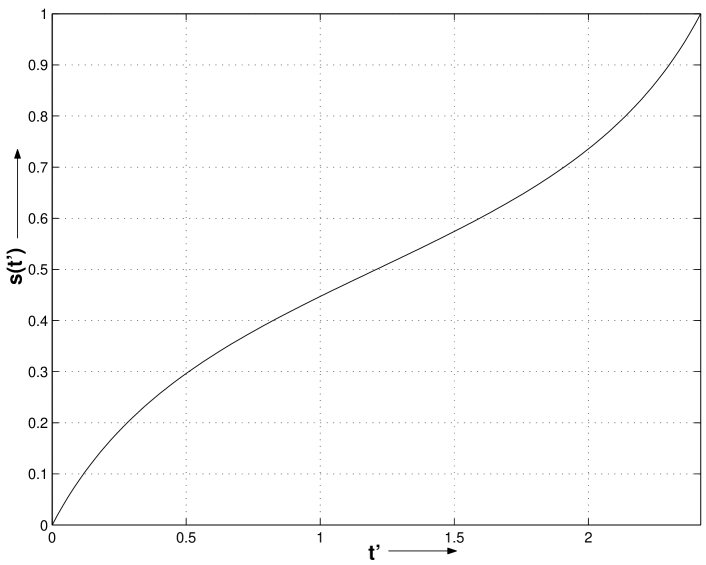
Figure 1:

(a)
(b)
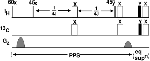
(c)
(d)
(e)
(f)

Figure 2:

Figure 3:

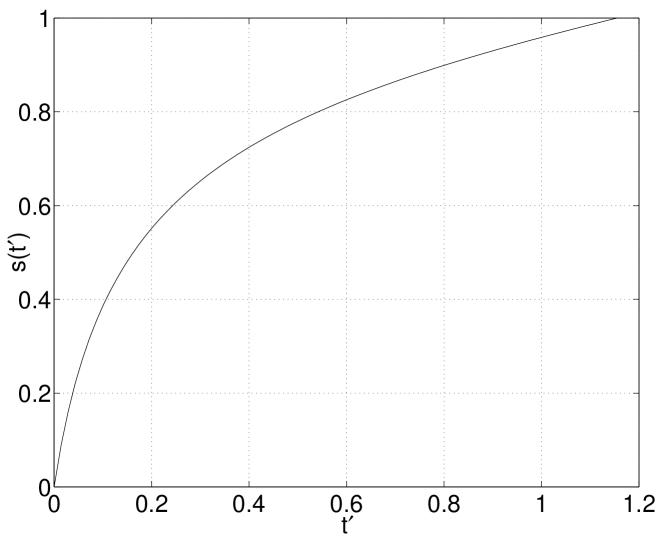
Figure 4:

Figure 5:

(a)
(b)

Figure 6:

Figure 7a:

Figure 7b:

(a)
(b)

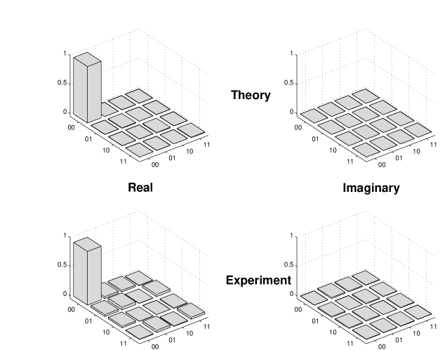
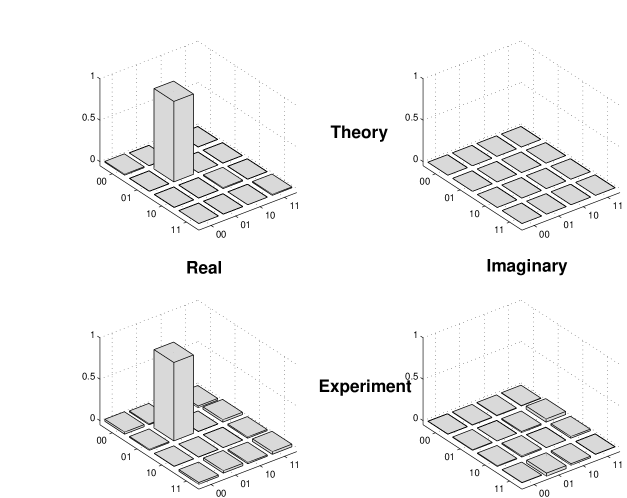
Figure 8:

(c)
(d)

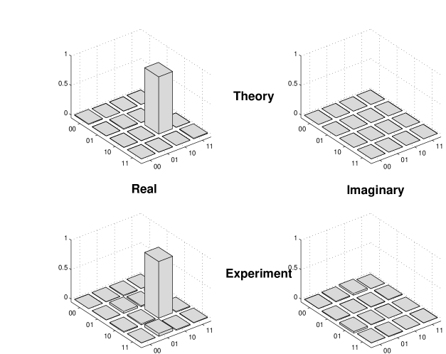
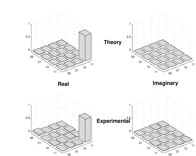
Figure 8: Cont.

(a)
(b)

Figure 9:

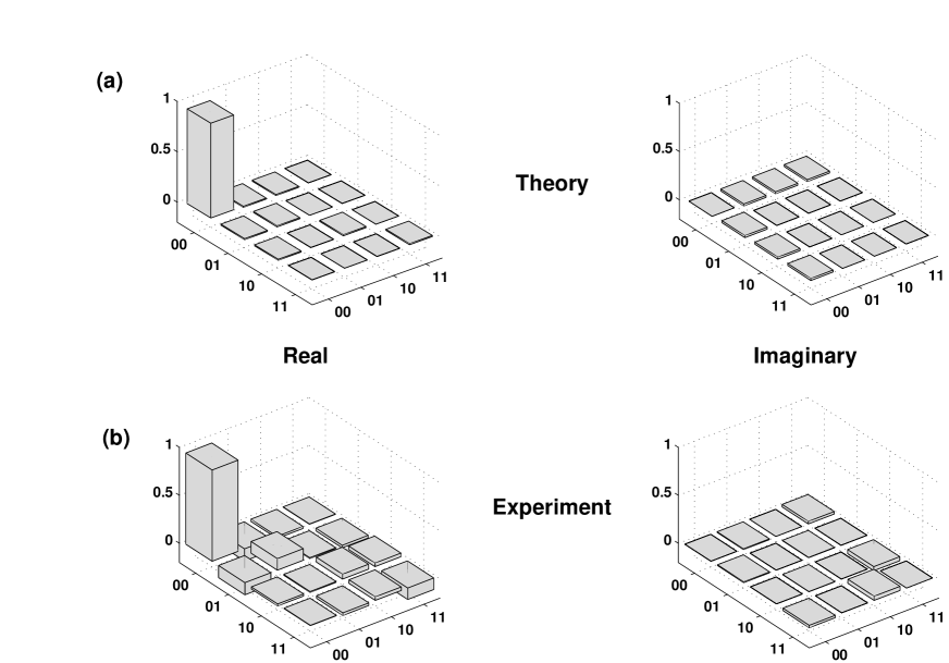
Figure 10:

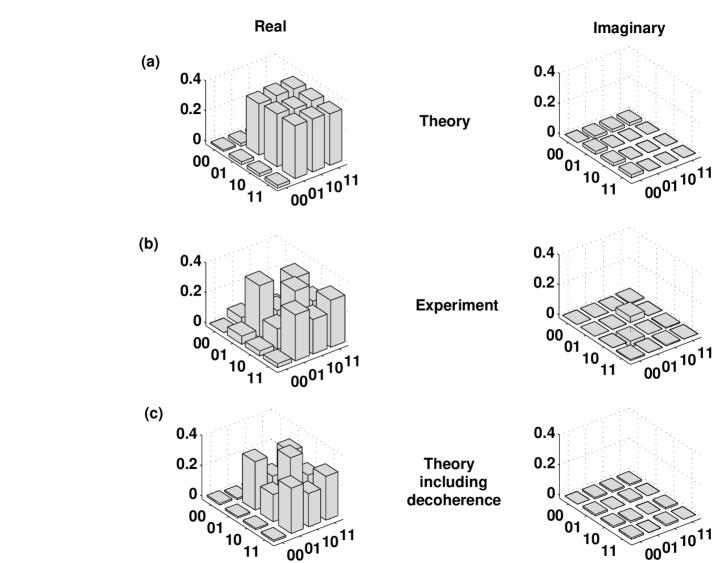
Figure 11:

References

-
(1)
J. Preskill, Lecture notes for Physics 229: Quantum information and Computation,
http://theory.caltech.edu/people/preskill . - (2) S. Lloyd, Science 273, 1073 (1996).
- (3) D. Deutsch and R. Jozsa, Proc. R. Soc. Lond. A 400, 97 (1985).
- (4) L.K. Grover, Phys. Rev. Lett. 79, (1997) 325.
- (5) P.W.Shor, SIAM Rev. 41, 303-332 (1999).
- (6) T. Hogg. Phys. Rev. Lett. 80, 2473 (1998).
- (7) E. Berstein and U. Vazirani, SIAM J. Computin. 26, 1411 (1997).
- (8) M. Boyer, G. Brassard, P. Hoyer, and A. Tapp. Fortschr. Phys. 46, 493 (1998).
- (9) D. Bouwnmeester, A. Ekert, A. Zeilinger(Eds.), ”The Physics of Quantum Information”, Springer, Berlin, 2000.
- (10) D. G. Cory, A.F. Fahmy and T.F. Havel, Proc.Natl.Acad.Sci. USA 94, 1634 (1997).
- (11) N. Gershenfeld and I.L. Chuang, Science 275, 350 (1997).
- (12) D. G. Cory, M. D. Price and T.F. Havel, Physica D, 120, 82 (1998).
- (13) I. L.Chuang, L. M. K. Vanderspyen, X. Zhou, D.W. Leung, and S. Llyod, Nature (London) 393, 1443 (1998).
- (14) J. A. Jones and M. Mosca, J. Chem. Phys. 109, 1648 (1998).
- (15) I. L. Chuang, N. Gershenfeld, and M. Kubinec, Phys. Rev. Lett. 80, 3408-3411 (1998).
- (16) J. A. Jones, M. Mosca and R. H. Hansen, Nature 393 344 (1998).
- (17) Kavita Dorai, T. S. Mahesh, Arvind and Anil Kumar, Current Science, 79 (10) 1447 (2000).
- (18) Kavita Dorai, Arvind, Anil Kumar, Phys Rev A. 61, 042306 (2000).
- (19) N. Sinha, T.S. Mahesh, K.V. Ramanathan and Anil Kumar, J. Chem. Phys. 114, 4415 (2001).
- (20) L.M.K. Vanderspyen, Matthias Steffen, Gregory Breyta, C.S.Yannoni, M.H. Sherwood and I.L. Chuang, Nature 414, 883 (2001).
- (21) Ranabir Das and Anil Kumar, Phys. Rev. A. 68, 032304 (2003).
- (22) Ranabir Das, A. Mitra, S. Vijaykumar and Anil Kumar Int. Jour. of Quant. Infor. 1(3) 387 (2003).
- (23) Ranabir Das, Sukhendu Chakraborty, K. Rukmani and Anil Kumar, Phys. Rev. A. (in press).
- (24) Ranabir Das, T.S. Mahesh and Anil Kumar, Phys. Rev. A. 67, 062304 (2003).
- (25) E. farhi, J. Goldstone, S. Guttmann, M. Sipser, quant-ph/0001106.
- (26) A. M. Childs, E. farhi, Phys. Rev. A, 65, 012322(2002).
- (27) E. farhi, J. Goldstone, S. Guttmann, J. Lapan, A. Lundgren, D. Preda, quant-ph/0104129.
- (28) A. M. Childs, E. farhi, J. Goldstone, S. Guttmann, Quant. Inf. Comp , 2, 181(2002).
- (29) E. farhi, J. Goldstone, S. Guttmann, quant-ph/0007071.
- (30) E. farhi, J. Goldstone, S. Guttmann, quant-ph/0208135.
- (31) M. R. Garey, D. S. Jhonson and L. Stockmeyer, Theor. Comput. Sci. 1, 237 (1976)
- (32) M. Steffen, Wim van Dam, T. Hogg, G. Bryeta, I. Chuang, Phys. Rev. Lett. , 90, 067903(2003).
- (33) S. Das, R. Kobes, G. Kunstatter, Phys. Rev. A, 65, 062310(2002).
- (34) A. Messiah, Quantum Mechanics, Vol II, Amsterdam: North Holland; New York:Wiley(1976).
- (35) Wim van Dam, M. Mosca, U. Vazirani, Proceedings of the 42nd Annual Symposium on Foundations in Coumputer Science, pp279-287(2001).
- (36) D.Deutsch, R. Jozsa, Proc. R. Soc. London A, 439, 553(1992).
- (37) J. Roland, N. J. Cerf, Phys. Rev. A, 65, 042308(2002).
- (38) J. Du, P. Zou, M. Shi, L. C. Kwek, Jian-Wei Pan, C. H. Oh, A. Ekert, D. K. L. Oi, and M. Ericsson, Phys. Rev. Lett. 91, 100403 (2003).
- (39) Principles of Nuclear Magnetic Resonance in One and Two Dimensions(Oxford University Press, New York, 1994).
- (40) G. Teklemariam, E. M. Fortunato, M. A. Pravia, T. F. Havel, D. G. Cory,Phys. Rev. Lett. ,86(2001),5845-5849
- (41) S. A. Smith, T. O. Levante, B. H. Meier and R. R. Ernst, J. Magn. Reson., 106a, 75-105, (1994).
- (42) W. H. Press, S. A. Teukolsky, W. T. Vetterling, B. P. Flannery, Numerical Recipies, 2nd ed. (Cambridge University Press, Cambridge, U.K., 1993).