Security of Quantum Key Distribution with Realistic Devices

Abstract

We simulate quantum key distribution (QKD) experimental setups and give out some improvement for QKD procedures. A new data post-processing protocol is introduced, mainly including error correction and privacy amplification. This protocol combines the ideas of GLLP and the decoy states, which essentially only requires to turn up and down the source power. We propose a practical way to perform the decoy state method, which mainly follows the idea of Lo’s decoy state. A new data post-processing protocol is then developed for the QKD scheme with the decoy state. We first study the optimal expected photon number $\mu$ of the source for the improved QKD scheme. We get the new optimal $\mu=O(1)$ comparing with former $\mu=O(\eta)$, where $\eta$ is the overall transmission efficiency. With this protocol, we can then improve the key generation rate from quadratic of transmission efficiency $O(\eta^{2})$ to $O(\eta)$. Based on the recent experimental setup, we obtain the maximum secure transmission distance of over 140 km.

Chapter 0 Introduction

Quantum key distribution (QKD) [1, 2] allows two parties, commonly called Alice, the transmitter and Bob, the receiver, to create a random secret key with the channel revealed to the eavesdropper, Eve. The security of QKD is built on the fundamental laws of physics in contrast to existing key distribution schemes that are based on unproven computational assumptions.

The best-known QKD scheme was proposed by Bennett and Brassard in 1984 (commonly called BB84 protocol) [1]. Alice uses a quantum channel, which is governed by quantum mechanics to transit single photons, each in one of four polarizations: horizontal ($0^{\circ}$), vertical ($90^{\circ}$), $45^{\circ}$, $135^{\circ}$. Bob randomly chooses one of two bases: rectangular ($+$) or diagonal ($\times$) to measure the arrived signals, and keeps the result privately. Consequently, Alice and Bob compare the bases they use and discard those in different bases. At last, Alice and Bob perform the local operations and classical communications (LOCC) to do the data post-processing, which is mainly composed of error correction and privacy amplification [3, 4, 5]. Our report will improve the procedure of BB84 with decoy state [6], [7] and apply the idea of GLLP [8] to develop a new post-processing protocol.

The security of the idealized QKD system has been proven in the past few years [9, 4, 5]. Now let us turn our attention to the experiment. Real setup is no longer ideal, but with imperfect sources, noisy channels and inefficient detectors, which will affect the security of the QKD system.

A weak coherent state is commonly used as the photon source, which is essentially a mixture of states with Poisson distribution of photon number. Thus, there is a non-zero probability to get a state with more than one photon. Then Eve may suppress the quantum state and keep one photon of the state that has more than one photon (commonly called multi photon, correspondingly, single photon denotes the state with only one photon). Moreover, Eve may block the single photon state, split the multi photon state and improve the transmission efficiency with her superior technologies to compensate the loss of blocking single photon. Without the technology to identify the photon numbers, Alice and Bob have to pessimistically assume all the states lost in the transmission and detection are single photons. In this way, the secure expected photon number $\mu$ of the signal state is roughly given by, $\mu=O(\eta)$, which implies that the key generation rate $R=O(\eta^{2})$, details can be found in section 3 and Appendix A.

The inefficiency of the detector will also affect the security of the QKD system. There exists a so-called dark count in the realistic detectors, which will increase the error rate of detection especially when the transmission efficiency is low. The dark count of a detector denotes the probability to get detection events when there is no input to the detector. Eve may use this imperfection to cover the error she introduces from her measurement of the single photon state.

In the recent paper GYS [10], the authors conducted an experiment in which the single photon was transmitted over 120 km. The question is whether the QKD experiment reported in GYS is secure or not? Unfortunately, based on the prior art of post-processing scheme, it is insecure. GYS uses the expected photon number $\mu=0.1$ as the source, which will be defeated by so-called photon number splitting attack in long distance. All in all, there exists a gap between the theory and experiment. Here, we are attempting to bridge the theory and experiment.

The key problem here is that Bob does not know whether his detection events come from: single photon, multi photon, or dark count. To solve this problem, we apply the idea of decoy state to learn the performance of single photon states. The decoy state here acts as a “scope” telling Alice and Bob which state comes from single photon, multi photon or dark count.

Our result is significant because it is a bridge between the theory and experiment of QKD. we extend the secure distance of the QKD system, increase the key generation rate substantially and maintain the major advantage of QKD — unconditional security. We improve the key generation rate from $O(\eta^{2})$ to $O(\eta)$. Notice that such a key generation rate is the highest order that any QKD system can achieve. Our improvement is mainly based on an advanced theory. We do not require any enhancement of equipment but only turning up and down the source power, which is easy to implement with current technology.

We notice that Koashi [11] has also proposed a method to extend the distance of secure QKD. It will be interesting to compare the power and limitations of our approach with that of Koashi.

The outline of this report is as follows. In section 1 we will recall to the proof of the security of an idealized QKD system with entanglement distillation protocol (EDP). In section 2, we shall review a couple of widely used QKD setups and simulates them following [12]. In section 3, we shall investigate the former post-processing schemes with the simulation and point out the limitation of prior art. We find out that the key generation rate $R$ is $O(\eta^{2})$, where $\eta$ is the overall transmission efficiency. In section 4, we combine the idea of GLLP [8] and decoy state [6, 7], and improve the key generation rate from $O(\eta^{2})$ to $O(\eta)$. In Appendix A, we discuss the choosing of the optimal expected photon number $\mu$, which maximizes the key generation rate. In Appendix B, we introduce a practical way to perform weak decoy state, which is a key step of the decoy state method.

Chapter 1 EDP schemes for QKD

In this section we will recall the security proof of the idealized QKD with EDP [13, 3, 14, 4]. The security of BB84 scheme can be reduced to the security of the Entanglement Distillation Protocol (EDP) schemes [5].

In the EDP protocol, Alice creates $n+m$ pairs of qubits, each in the state

$$|\psi\rangle=\frac{1}{\sqrt{2}}(|00\rangle+|11\rangle),$$

the eigenstate with eigenvalue $1$ of the two commuting operators $X\bigotimes X$ and $Z\bigotimes Z$, where

$$X=\begin{pmatrix}0&1\\ 1&0\\ \end{pmatrix},Z=\begin{pmatrix}1&0\\ 0&-1\\ \end{pmatrix}$$

are the Pauli operators. Then she sends half of each pair to Bob. Alice and Bob sacrifice $m$ randomly selected pairs to test the error rates in the $X$ and $Z$ bases by measuring $X\bigotimes X$ and $Z\bigotimes Z$. If the error rate is too high, they abort the protocol. Otherwise, they conduct the EDP, extracting $k$ high-fidelity pairs from the $n$ noisy pairs. Finally, Alice and Bob both measure $Z$ on each of these pairs, producing a k-bit shared random key about which Eve has negligible information. The protocol is secure because the EDP removes Eve’s entanglement with the pairs, leaving her negligible knowledge about the outcome of the measurements by Alice and Bob.

A QKD protocol based on a CSS-like EDP can be reduced to a “prepare-and-measure” protocol [5]. CSS code [15] conducts error correction to the bit error and the phase error separately. That is to say, CSS-like EDP deals with the error correction and privacy amplification separately, which can be further improved by two-way communication [16]. Thus the residue of this data post-processing protocol is the so-called CSS rate,

$$\eta_{post}^{CSS}=1-H_{2}(\delta_{b})-H_{2}(\delta_{p})$$ (1)

where $\delta_{b}$ and $\delta_{p}$ are the bit flip error rate and the phase flip error rate, and $H_{2}(x)$ is binary Shannon information function,

$$H_{2}(x)=-x\log_{2}(x)-(1-x)\log_{2}(1-x).$$

In summary, there are two main parts of EDP, bit flip error correction (for error correction) and phase flip error correction (for privacy amplification). These two steps can be understood as follows. First Alice and Bob apply bi-direction error correction, after which they share the same key strings but Eve may still keep some information about the key. Alice and Bob then perform the privacy amplification to expunge Eve’s information from the key. The final key will be secure if the privacy amplification is successfully done in principle. That is Alice and Bob do not need to actually do the privacy amplification but only ensure that this can be done. In practice, Alice and Bob can calculate the residue of the privacy amplification and perform random hashing to get the final key with high security.

Chapter 2 Simulations for experiments

To simulate a real-life QKD system, we need to model the source, channel and detector. In this section, we first review the real experimental setup, and then simulate the QKD system following [12], at last verify the simulation with real experimental data.

1 QKD setup

Let us recall the principle of the so-called p&p auto-compensating setup [17, 18], where the key is encoded in the phase between two pulses trading from Bob to Alice and back (see Fig. 1). A strong laser pulse emitted from Bob is separated by a first 50/50 beam splitter (BS). The two pulses impinge on the input ports of a polarization beam splitter (PBS), after having traveled through a short arm and a long arm, including a phase modulator ($PM_{B}$) and a delay line (DL), respectively. All fibers and optical elements at Bob are polarization maintaining. The linear polarization is rotated by $90^{\circ}$ in the short arm, therefore the two pulses exit Bob’s setup by the same port of the PBS. The pulses travel down to Alice, are reflected on a Faraday mirror, attenuated, and come back orthogonally polarized. In turn, both pulses now take the other path at Bob and arrive at the same time at the BS where they interfere. Then, they are detected either in $D_{1}$, or after passing through the circulator (C) in $D_{2}$. Since the two pulses take the same path, inside Bob in reversed order, this interferometer is auto-compensated.[18]

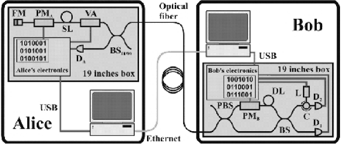
Figure 1: Schematic of the p&p prototype. This figure comes from [18]

To implement the BB84 protocol, Alice applies a phase shift of $0$ or $\pi$ and $\pi/2$ or $3\pi/2$ on the second pulse with $PM_{A}$. Bob chooses the measurement basis by applying a $0$ or $\pi/2$ shift on the first pulse on its way back.[18]

As for the free-space QKD system, the setup is easier. There are only encoded signals which come from Alice’s side to Bob’s, comparing with the p&p setup, the pulses traveling from Bob to Alice and back. In this sense, the free-space setup is closer to the original BB84 schemes. More details of this kind of QKD setup can be found in [19, 20, 21].

2 Modeling the real-life QKD system

Following prior papers such as [12], we simulate the p&p QKD system. The first important parameter for the real-life QKD system is the key bit rate $B$ between Alice and Bob. More explicitly, $B$ is the number of exchanged key bits per second, given by

$$B=\nu R,$$ (1)

where $\nu$ is the repetition frequency in Alice’s side, and $R$ is the key generation rate, i.e. the number of exchange bits per pulse, given by

$$R=qp_{D}\eta_{post},$$ (2)

where $q$ depends on the implementation (1/2 for the BB84 protocol, because half the time Alice and Bob disagree with the bases, and if one uses the efficient BB84 protocol [22], one can have $q\approx 1$), $p_{D}$ is the average number of signals per pulse detected by Bob, and $\eta_{post}$ denotes for the residue of data post-processing, i.e. the efficiency of error correction and privacy amplification, which is also discussed in section 1 Eq. (1). We will study $p_{D}$ in the following and discuss $\eta_{post}$ in the section 3 and 4.

For optical fibers, the losses in the quantum channel can be derived from the loss coefficient $\alpha$ measured in dB/km and the length of the fiber $l$ in km. The channel transmission $t_{AB}$ can be expressed as

$$t_{AB}=10^{-\frac{\alpha l}{10}}.$$

Let $\eta_{Bob}$ denote for the internal transmission $t_{Bob}$ and detection efficiency $\eta_{D}$ in Bob’s side, given by

$$\eta_{Bob}=t_{Bob}\eta_{D}.$$

Then the overall transmission and detection efficiency between Alice and Bob $\eta$ is given by

$$\eta=t_{AB}\eta_{Bob}.$$ (3)

The average number of signals per pulse detected by Bob, i.e. the probability for Bob to get a signal from his detector $p_{D}$, is given by

$$p_{D} =p_{Signal}+p_{dark}-p_{Signal}p_{dark}$$ (4)

$$\cong p_{Signal}+p_{dark},$$

where we assume that the dark counts are independent of the signal photon detection. $p_{dark}$ and $p_{Signal}$ are the probabilities to get a dark count and to detect a photon originally emitted by Alice respectively.

The dark count depends on the characteristics of the photon detectors. The effect of dark count will be significant when $\eta\mu$ is small which implies $p_{Signal}$ is small. It is necessary to point out that $p_{dark}$ is the overall dark count throughout the QKD system. Here we consider the p&p QKD setup, $p_{dark}$ is twice as large as $d_{B}$ because there are two sources of dark count, i.e. two detectors in the QKD system. Then the $p_{dark}$ is given by

$$p_{dark}=2d_{B},$$

where $d_{B}$ denotes the dark count of one detector.

Normally, a weak coherent state is used as the signal source. Assuming that the phase of this signal is totally randomized, the number of photons of the signal state follows a Poisson distribution with a parameter $\mu$ as its expected photon number. In appendix B, we will discuss the optimal value of expected photon number $\mu$ which optimizes the key generation rate $R$. $p_{Signal}$ is given by

$$p_{Signal}=\sum_{i=1}^{\infty}\eta_{i}\cdot\frac{\mu^{i}}{i!}\exp(-\mu),$$ (5)

where $\eta_{i}$ is the transmission efficiency of i-photon state in a normal channel. It is reasonable to assume independence between the behaviors of the $i$ photons. Therefore the transmission efficiency of i-photon state $\eta_{i}$ is given by

$$\eta_{i}=1-(1-\eta)^{i}.$$ (6)

Substitute (6) into (5), we have,

$$p_{Signal} =\sum_{i=1}^{\infty}[1-(1-\eta)^{i}]\cdot\frac{\mu^{i}}{i!}\exp(-\mu)$$ (7)

$$=1-\exp(-\eta\mu).$$

We can divide $p_{Signal}$ into two parts $p_{S}$ and $p_{M}$, which are the probabilities of single photon and multi photon states emitted from Alice’s side that are detected by Bob. Then (4) is given by,

$$p_{D} =p_{dark}+p_{S}+p_{M}$$ (8)

$$=p_{dark}+1-e^{-\eta\mu}.$$

The overall quantum bit error rate (QBER, denoted by $\delta$) is an important parameter for error correction and privacy amplification $\eta_{post}$. QBER is equivalent to the ratio of the probability of getting a false detection to the total probability of detection per pulse. It comes from three parts: dark count, single photon and multi photon,

$$\delta =\frac{\frac{1}{2}p_{dark}+\delta_{S}p_{S}+\delta_{M}p_{M}}{p_{D}},$$ (9)

where $\delta_{S}$ and $\delta_{M}$ denote the error rate of single and multi photon detection, respectively. The dark counts occur randomly, thus the error rate of dark count is $\frac{1}{2}$.

Due to the high loss in the channel, the multi photon states arriving at Bob’s side always has only one photon left. Thus, we have the similar probability of erroneous detection for single photon and multi photon. The bit error rate $\delta_{S}$ and $\delta_{M}$ are given by,

$$\delta_{M}\cong\delta_{S}=e_{detector},$$ (10)

where $e_{detector}$ is the probability that a photon hit the erroneous detector. $e_{detector}$ characterizes the quality of the optical alignment of the polarization maintaining components and the stability of the fiber link [18]. It can be measured with strong pulses, by always applying the same phases and measuring the ratio of the count rates at the two detectors. In our discussion, we neglect $e_{detector}$’s dependence of the fiber length because the change of alignment during the transmission of a signal is very small.

Substituting (10) into (9), QBER is given by,

$$\delta=\frac{\frac{1}{2}p_{dark}+e_{detector}p_{Signal}}{p_{D}}.$$ (11)

There is another important parameter for privacy amplification, the ratio of single photon detection in overall detection events $f_{1}$ which is defined by,

$$f_{1}=\frac{p_{S}}{p_{D}}.$$ (12)

Only the key extracted from the single photon state can be secure. Thus, $f_{1}\cdot p_{D}$ roughly gives the upper bound of the key generation rate.

3 Verify the simulation by QBER

Here we would like to verify the equations (11) by comparing the experimental result and our simulation. The parameters of the experimental setup are listed in Tab. 1.

	T8[23]	G13[24]	KTH[25]	GYS[10]
Wavelength [nm]	830	1300	1550	1550
$\alpha$ [dB/km]	2.5	0.32	0.2	0.21
$t_{B}$ [dB]	8	3.2	1	5*
$e_{detector}$ [%]	1	0.14	1	3.3
$d_{B}$ [per slot]	$5\times 10^{-8}$	$8.2\times 10^{-5}$	$2\times 10^{-4}$	$8.5\times 10^{-7}$
$\eta_{D}$ [%]	50	17	18	12*

Table 1: Key parameters for p&p QKD experiment setup. * GYS gives out that $\eta_{Bob}=0.045$.

Fig. 2 shows QBER as a function of expected photon number $\mu$. For $\mu$ valuing in the range $10^{-1}\sim 10^{-4}$, the QBER has a constant value of about $1\%$ that is dominated by depolarization-induced errors $e_{detector}$. These errors arise from dynamic depolarization that results from the finite extinction ratios of the various polarizing components in the system [23]. For $\mu<10^{-4}$ the QBER rises as the dark counts falling within the detectors start to become the dominant contribution to the noise.

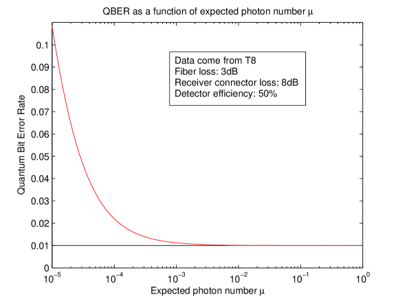
Figure 2: shows QBER as a function of input expected photon number using Eq. (11), reproducing T8’s Fig 3. The key parameters are, according to T8 [23], listed in Tab. 1, and the fiber loss is 3dB ($\sim 1.5$km).

Fig. 3 shows QBER as a function of transmission distance using Eq. (11). In the long distance ($l>100km$, say), the QBER rises as the dark counts become the dominant contribution to the noise. Note the exponential dependence is due to the loss of photons in the propagation, referring to $p_{Signal}$ of Eq. (7). If stronger source (say, $\mu=0.5$) is used, QBER will be lower, especially in the long distance region.

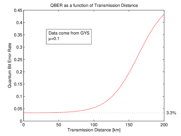
Figure 3: shows QBER as a function of the transmission distance, using the Eq. (11). This is a reproduction of FIG.3 in GYS’ paper [10]. The key parameters are, according to GYS [10], listed in Tab. 1. The expected photon number $\mu$ is 0.1.

From these verifications, we can see that the Eq. (11) fits the experiment well, so the simulation is accurate.

Chapter 3 Our comparison of Prior Art Results

Now, we begin to examine the relationship between key generation rate $R$ and the transmission distance with prior QKD data post-processing schemes. Two ideas in Lütkenhaus’ paper [12] and GLLP’s paper [8] are compared. Note that it is our new work to calculate the key generation rate $R$ with the experimental simulation using the idea of GLLP [8].

In both papers, the authors are going on the assumption that all of the photons that fail to arrive were emitted as single photons. Later, we will improve this point by introducing the decoy states scheme. Assuming that,

$$p_{M}=S_{M},$$ (1)

where $S_{M}$ is the probability of emitting a multi photon state from Alice’s side, which is dependent on attribute of the source. Based on the Poisson distribution of the number of photons of the signal states,

$$S_{M}=1-(1+\mu)\exp(-\mu).$$

Another assumption used here is that all the error (QBER) comes from the single photon state. Then the error rate of single photon is given by,

$$\delta_{S}=\frac{\delta}{f_{1}}.$$ (2)

For individual attacks, the residue of error correction and privacy amplification can be given by [12],

$$\eta_{post}= \max\{f_{1}(1-\log_{2}[1+\frac{4\delta}{f_{1}}-4(\frac{\delta}{f_{1}})^{2}])$$ (3)

$$-f(\delta)H_{2}(\delta),0\},$$

where $f(\delta)\geq 1$ is the efficiency of error correction [26] listed in Tab. 1, $\delta$ is the QBER given in equation (11), $f_{1}$ is defined in (12).

$\delta$	0.01	0.05	0.1	0.15
f($\delta$)	1.16	1.16	1.22	1.35

Table 1: The data come from [12]. The author used used the upper bounds for I(4) provided in [26].

We would like to explain the idea of GLLP’s [8] tagged state briefly here. Notice the idea of tagged state is (perhaps implicitly) introduced by [27]. In principle, one can separate the tagged and untagged states, i.e. one can do random hashing for the privacy amplification on the tagged state and untagged state separately. Therefore, the data post-processing can be performed as following. First, apply error correction to the overall states, sacrificing a fraction $H_{2}(\delta_{b})$ of the key, which is represented in the first term of formula (4). After correcting errors in the sifted key string, one can imagine executing privacy amplification on two different strings, the sifted key bits $s_{tagged}$ arising from the tagged qubits and the sifted key bits $s_{untagged}$ arising from the untagged qubits. Since the privacy amplification [8] is linear (the private key can be computed by applying the $C_{2}$ parity check matrix to the sifted key after error correction), the key obtained is the bitwise $XOR$

$$s_{untagged}\oplus s_{tagged}$$

of keys that could be obtained from the tagged and untagged bits separately. If $s_{untagged}$ is private and random, then it doesn’t matter if Eve knows everything about $s_{tagged}$ — the sum is still private and random. Therefore we ask if privacy amplification is successful applied to the untagged bits alone. Thus, the residue after error correction and privacy amplification can be expressed as,

$$\eta_{post}=\max\{-f(\delta)H_{2}(\delta)-f_{1}(1-H_{2}(\frac{\delta}{f_{1}})),0\}.$$ (4)

Here the single photon state is regarded as the untagged state and its error rate ($\delta_{b}=\delta_{p}$) is given by (2).

Based on (2), (3) and (4), according to Appendix B, the optimal expected photon number $\mu$, which maximizes the key generation rate, is roughly given by,

$$\mu\approx\eta,$$ (5)

where $\eta$ is the overall transmission, defined in the (3). Therefore, the key generation rate is given by,

$$R=O(\eta\mu)=O(\eta^{2}).$$ (6)

Now, use (5) as the expected photon number to calculate the key generation rate of two different schemes by equation (3) and (4) with Lütkenhaus’ and GLLP’s post-processing protocols.

Fig. 1 shows the relationship between key generation rate and the transmission distance by one-way LOCC, comparing Lütkenhaus’ individual attack and GLLP’s general attack case. From the Fig. 1, we can see that GLLP is only slightly worse than Lütkenhaus’, but GLLP deal with the general attack while Lütkenhaus’ result is restricted in individual attack. Our result shows that there seems to be little to be gained in restricting security analysis to individual attacks, given that the two papers—Lütkenhaus vs GLLP—gave very similar results. In other words, our view is that one is better off in considering unconditional security, rather than restricting one’s attention to a restricted class of attacks (such as individual attacks). Note that the key generation rate $R$ of GYS with GLLP will strictly hit 0 at distance $l=34km$.

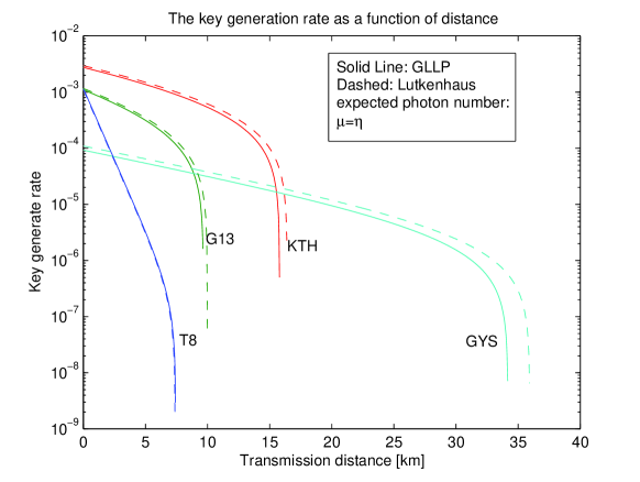
Figure 1: shows the relationship between key generation rate and the transmission distance, comparing Lütkenhaus’ individual attack and GLLP’s general attack case. The key parameters are listed in Tab. 1. It is our new work to calculate the key generation rate $R$ with the experiment simulation using the idea of GLLP [8].

Chapter 4 Decoy state method

So far as discussed, the prior art gives Eve many ideal advantages such as she can make the tagged state no error and no loss in the channel, however, this is not necessary. We can control Eve’s performance on tagged states by adding decoy states. “Control” does not mean limit the quantum or classical computation ability of Eve, but means we can detect Eve if she uses some eavesdropping strategies to enforce the tagged states.

1 The idea of decoy state

The decoy state method is proposed by Hwang [6] and further studied by [7]. The idea is that, by adding some decoy states, one can estimate the behavior of vacua, single photon states, and multi photon states individually.

The key point is that, with the decoy state, Alice and Bob can gain photon number information which cannot be derived by today’s technologies directly. They can use this extra information to “detect” the behavior of states with different photon numbers. Eve cannot distinguish whether the photon comes from signal state or decoy state. Thus, the transmission efficiency $\{\eta_{i}\}$, detection probabilities and error rates ($\delta_{S}$, $\delta_{M}$) in the signal state will be the same as those in decoy state,

$$\eta_{i}(Signal) =\eta_{i}(Decoy)$$

$$\delta_{S}(Signal) =\delta_{S}(Decoy)$$

$$\delta_{M}(Signal) =\delta_{M}(Decoy),$$

where $i=1,2,3\cdots$.

Our decoy state method is quite different from Hwang’s original one. Hwang uses strong pulse as decoy state. We mainly follow [7]’s decoy idea, using vacua and very weak state as decoy states.

2 Simulation with new assumption

With the decoy states, we can drop the “pessimistic” assumption (1). According to Poisson distribution of photon source, the single photon and multi photon detection probabilities are given by

$$p_{S}=\eta\mu\exp(-\mu)$$ (1)

$$p_{M} =\sum_{i=2}^{\infty}[1-(1-\eta)^{i}]\frac{\mu^{i}}{i!}e^{-\mu}$$ (2)

$$=1-e^{-\eta\mu}-\eta\mu e^{-\mu},$$

where $\mu$ is the expected photon number and $\eta$ is the overall transmission and detection efficiency, defined in (3). The transmission efficiency of an i-photon state $\eta_{i}$ is given by (6).

We remark that the Eqs. (1) and (2) do not consider dark count contributions. In real-life, dark count contributions must be included. Therefore, following Eq. (4), we write down the total contribution (true signals plus dark counts) as follows,

$$\tilde{p}_{dark} =p_{dark}e^{-\mu}$$ (3)

$$\tilde{p}_{S} =p_{S}+p_{dark}\mu e^{-\mu}$$

$$\tilde{p}_{M} =p_{M}+p_{dark}[1-(1+\mu)e^{-\mu}]$$

and the error rate of dark count is still $\frac{1}{2}$, for single photon and multi photon,

$$\tilde{\delta}_{S} =\frac{\frac{1}{2}p_{dark}+e_{detector}p_{S}}{p_{dark}+p_{S}}$$ (4)

$$\tilde{\delta}_{M} =\frac{\frac{1}{2}p_{dark}+e_{detector}p_{M}}{p_{dark}+p_{M}}.$$

3 A way to perform decoy state

Here we would like to introduce a specific method to perform decoy state, which is proposed by [7]. There are three kind of signals Alice and Bob should perform.

First, Alice and Bob can study the dark counts by using vacua as decoy states. Here we reasonably assume that the density matrix of dark counts is the identity matrix. Thus, in theory, they will detect the probability to get a signal $p_{D}^{vacua}$ and the overall error rate $\delta^{vacua}$,

$$p_{D}^{vacua} =p_{dark}=2d_{B}$$ (5)

$$\delta^{vacua} =\frac{1}{2}.$$

They can measure $p_{D}^{vacua}$ and $\delta^{vacua}$ via experimental methods and then compare with the Eq.(5). If the experimental results match the Eq.(5), then keep going. Otherwise, they need to check out the QKD system setup, especially the detectors.

Secondly, Alice and Bob can get the transmission and the bit flip error rate of the single photon state by using very weak coherent states as decoy states. With weak decoy state, according to (8) and (11), $p_{D}^{weak}$ and $\delta^{weak}$ are given by,

$$p_{D}^{weak} =p_{dark}+p_{S}^{weak}+p_{M}^{weak}$$ (6)

$$\delta^{weak} =\frac{\frac{1}{2}p_{dark}+\delta_{S}p_{S}^{weak}+\delta_{M}p_{M}^{weak}}{p_{D}^{weak}},$$

where the superscript weak denotes the value comes from weak decoy state. In appendix B, we will discuss the how to choose $\mu^{weak}$ in practice.

If the decoy state is weak enough, i.e. $\mu^{weak}\ll 1$, at which value

$$\frac{p_{M}^{weak}}{p_{S}^{weak}}=O(\mu^{weak})\ll 1,$$ (7)

we can neglect the multi photon terms in Eq.(6). After that we have

$$p_{S}^{weak}=p_{D}^{weak}-p_{dark},$$

and substitute this formula into (3), (4),

$$\tilde{p}_{S}^{weak} =p_{D}^{weak}-p_{dark}(1-\mu^{weak}e^{-\mu^{weak}})$$ (8)

$$\cong p_{D}^{weak}-p_{dark}e^{-\mu^{weak}}$$

$$\tilde{\delta}_{S} \cong\frac{\delta_{weak}p_{D}^{weak}-\frac{1}{2}p_{dark}e^{-\mu^{weak}}}{p_{S}^{weak}}$$

where $p_{dark}$ can be derived from the Eq.(5), and $p_{D}^{weak}$, $\delta_{weak}$ can be obtained from the experiment.

Thirdly, Alice and Bob perform the signal state, where the final key is drawn from. The detection probability $p_{D}$ and QBER $\delta$ are given by (8) and (11).

4 Data post-processing

Here, we would like to discuss the data post-processing for QKD with the decoy state, mainly based on [8].

We can further extend the GLLP’s idea [8], as discussed in section 3, to more than one kind of tagged states case, i.e. several kinds of states with flag $g$. The procedure of data post-processing is similar, do the overall error correction first and then apply the privacy amplification to each case. At last the residue of error correction and privacy amplification is given by,

$$\eta_{post}=\max\{-f(\delta_{b})H_{2}(\delta_{b})+\sum_{g}p^{g}[1-H_{2}(\delta_{p}^{g})],0\}$$ (9)

where one need to sum over all cases with flag $g$, $p^{g}$ is the probability of the case with flag $g$ and $\delta_{p}^{g}$ is the phase flip error rate of the state with flag $g$

In order to combine the ideas of GLLP and Decoy, we should find out all parameters for Eq. (9). There are three kind of states in the discussion, dark count, single photon, and multi photon. The multi photon state emitting out of the source can be expressed by $|000\rangle+|111\rangle$. After Eve gets the extra photon, the state will be a mixture of $|00\rangle+|11\rangle$ and $|00\rangle-|11\rangle$ with the same probability. Thus the phase flip error rate for multi photon will be $\frac{1}{2}$. In addition to the discussion in 2, we can list the bit flip error rate $\delta_{b}$ and phase flip error rate $\delta_{p}$ for dark count, single photon and multi photon in Tab. 1.

	Dark count	Single Photon	Multi Photon
$\delta_{b}$	$\frac{1}{2}$	$\tilde{\delta}_{S}$	$\tilde{\delta}_{M}$
$\delta_{p}$	$\frac{1}{2}$	$\tilde{\delta}_{S}$	$\frac{1}{2}$

Table 1: Bit flip error rate and phase flip error rate for different kinds of photon state.

Apply above idea, Eq. (9), to decoy states scheme with the parameters listed in Tab. 1. We get the formula for post-processing residue,

$$\eta_{post}=\max\{-f(\delta_{b})H_{2}(\delta_{b})+\frac{\tilde{p}_{S}}{p_{D}}[1-H_{2}(\tilde{\delta}_{S})],0\}$$ (10)

where $\tilde{p}_{S}$ and $\tilde{\delta}_{S}$ are given by (3), (4). Note that the dark count and multi photon state have no contribution to the final key with phase flip error rate $\delta_{p}=\frac{1}{2}$. The reason why we use $\tilde{p}_{S}$ and $\tilde{\delta}_{S}$ here is that Bob cannot distinguish the detection event from real signal or dark count. And substitute (10) into the equation (2), if the key generation rate is $R>0$,

$$R=\frac{1}{2}\{-p_{D}f(\delta)H_{2}(\delta)+\tilde{p}_{S}[1-H_{2}(\tilde{\delta}_{S})]\}$$ (11)

where $\delta$ is the overall QBER given in (11).

Through the analysis in Appendix B, we have, for the KTH [25] experimental setup,$\mu_{Optimal}\approx 0.8$ and for GYS [10], $\mu_{Optimal}\approx 0.5$. Therefore, the key generation rate is given by,

$$R=O(\eta\mu)=O(\eta)$$ (12)

The result is shown in Fig.1.

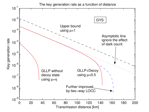
Figure 1: shows the key generation rate as a function of the transmission distance, GLLP+Decoy Eq. (11). The key parameters are listed in Tab. 1 and f(e) is given by Tab. 1. We use linear regression for f(e).

Remarks for the figure:

1. The dashed line is the upper bound of the key generation rate. The key generation rate here is derived from the photon detection events of Bob that occur when Alice sends single photon signals. It is to say, Bob can distinguish dark count, single photon, and multi photon. In this way the upper bound of key generation rate is given by,

   $$R_{max}=Q_{1}(1-H_{2}(e_{detector})).$$

   It is obvious that the optimal expected photon number for the upper bound is $\mu=1$. The gap between the upper bound and the decoy curve shows how much room is left for improvements of data post-processing.

2. The dotted line is the asymptotic line that neglects the influence of dark count, which is given by,

   $$R_{Asym}= -p_{D}f(e_{detector})H_{2}(e_{detector})$$

   $$+p_{S}[1-H_{2}(e_{detector})]$$

   $$p_{D}= 1-\exp(\eta\mu),$$

3. The “decoy” and “without decoy” line will hit zero at some points. This can be seen from the formula (11), $R=0$ when,

   $$-Q_{Signal}f(E_{Signal})H_{2}(E_{Signal})$$

   $$+Q_{1}[1-H_{2}(\delta_{S})]\leq 0.$$

   From the program (as shown in figure), when $l=144km$ for GLLP+Decoy, and $l=34km$ for GLLP, $R$ will hit 0.

4. One can further improve the data post-processing protocol with two-way LOCC [16]. As shown in Fig.1, dashed curve outside of decoy curve, two-way LOCC improve the maximum distance by about 20 km.

Compare the curves with and without decoy, we can find that the advantages of decoy state are obvious,

1. The initial key generation rate (at zero distance) is substantially higher with decoy state than without. It is because a stronger source (higher $\mu$) is used in the decoy state scheme.

2. At short distances, the key generation rate decreases with distance exponentially mainly due to exponential losses in the channel. The two curves, with and without decoy state behave like straight lines. Note that the initial slope without decoy is twice of that with decoy state. This is because without decoy state, $R=O(\eta^{2})$, while with decoy state, $R=O(\eta)$ according to (6) and (12).

3. Suppose $10^{-6}$ is the cut-off point for key generation rate. The two curves intercept the cut-off point at rather different locations (with decoy: 139 km, and without decoy: 31 km). For GYS, the distance is over 100km. It is comparable to the distance between amplifiers in optical metropolitan area networks (MANs).

Here, we would like to discuss the key bit rate $B$, which is different from behavior with key generation rate $R$ only with a constant, repetition frequency, according to Eq. (1). It is necessary to point out that there are two repetition frequencies in real-life setups: the source frequency $\nu_{A}$, which is the limitation of signal source repetition at Alice’s side and the detection rate $\nu_{B}$, which is the limitation of detector’s count rate in Bob’s side. There are two cases we should consider. First, when the overall transmission loss is not too large, the detection frequency $\nu_{B}$ limits the final key bit rate, because we can complement the loss in the transmission through increasing the source frequency $\nu_{A}$ until reaches $\nu_{A}$’s maxima. In this case, $B$ is simply given by, $B=\nu_{B}$. Secondly, when the overall transmission loss is large, $B$ is determined by the source rate $\nu_{A}$. Then the key bit rate $B$ is given by (1), $B=\nu_{A}R$.

We remark that the decoy state idea can also be used for free-space QKD setup [28]. The simulation of the setup will be similar.

Conclusion

In this report, we have presented a security proof of quantum cryptography against the general attack with real-life devices. We have formulated a method for estimating the key generation rate in the presence of realistic devices by combining the idea of decoy state and GLLP. The model has been applied to various real-life experimental setups. Based on recent experiment results, secure transmission distance of the QKD system can be up to 140 km.

We have improved the key generation rate substantially. The main reason for this improvement is that with decoy state we can choose the expected photon number $\mu$ of source in the order of O(1), while without decoy state, $\mu=O(\eta)$. With the decoy state, a new data post-processing protocol is developed, which essentially comes from the idea of GLLP. We have also proposed a pratical way to fulfills the ideal of decoy state as discussed in section 3 and Appendix B. In this sense, it can help to design the QKD procedure.

Through the simulation, it is clearly shown that, in order to improve the transmission distance, one should reduce the dark count and fiber loss in the channel; as for the aim of higher key bit rate, we should increase the detection repetition or reduce the errors in the transmission.

Chapter 5 Appendix A

In this section, we will discuss the choosing of the expected photon number $\mu$ for different error correction and privacy amplification schemes in section 3, 4. We will discuss the optimal $\mu$ generally and then work out reasonable value for each scheme.

We would like to start with generic discussion. On one hand, we need to maximize the probability of single photon detection, which is the only source for the final key. To achieve this point, we should maximize the single photon sources since transmission efficiency is fixed. Considering the real photon sources, according to Poisson distribution of the photon number, the single photon source reaches its maximum when $\mu=1$. On the other hand, we have to control the probability of multi photon detection to ensure the security of the system. On this side, we should keep the tagged states ratio ($1-f_{1}$) small, which requires $\mu$ not too large. It follows that $\mu\leq 1$, because based on both points, the case of $\mu>1$ is always worse than the case of $\mu=1$, And another parameter should be considered is the QBER $\delta$, which is decrease when $\mu$ increases, according to the formulas (11). Therefore, intuitively we have that,

$$\mu\in(0,1].$$

1 Without decoy state

Here, we would like to consider the case without decoy state, i.e. GLLP and Lütkenhaus’s cases. A similar discussion is given in [12]. We desire to get an optimal value of $\mu$ that maximizes the key generation rate $R$ with other parameters fixed. The key parameters here are the overall transmission and detection efficiency $\eta$, dark count $d_{B}$, and the probability of erroneous detection $e_{detector}$, which are specified by various setups.

In the R-distance figures, such as Fig. 1 and 1, the key generation rate drops roughly exponentially with the transmission distance before it starts to drop faster due to the increasing influence of the dark counts. The initial behavior is mainly due to the multi-photon component of the signals while the influence of the error-correction part is small. In this regime we can bound the gain by the approximation

$$R \leq\frac{1}{2}(p_{Signal}-p_{M})$$

$$=\frac{1}{2}[(1+\mu)\exp(-\mu)-\exp(-\eta\mu)]$$

with the pessimistic assumption (1). This expression is optimized if we choose $\mu=\mu_{Optimal}$, which fulfills

$$-\mu\exp(-\mu)+\eta\exp(-\eta\mu)=0.$$

Since for a realistic setup we expect that $\eta\mu\ll 1$, we find

$$\eta_{Optimal}\approx\eta.$$ (1)

Now, we can use the numerical analysis to verify the formula (1). When we keep all parameters fixed and vary the expected photon number $\mu$ of the signal, then we can use dichotomy method to find out the $\mu_{Optimal}$, which maximizes the key generation rate by the formula (2) and (4). If we fix the dark count $d_{B}$ and the probability of erroneous detection $e_{detector}$, and vary the transmission efficiency $\eta$ we can draw the relationship between the optimal $\mu_{Optimal}$ and $\eta$. The result is shown in Fig. 1, from which we can clearly see that the formula (1) is a good approximation.

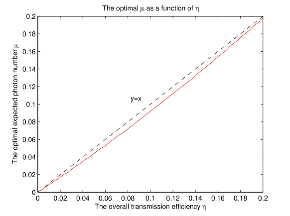
Figure 1: Optimal expected photon number $\mu$ as a function of transmission efficiency $\eta$, with the parameters listed in Tab. 1, T8 [23]. Here, we use dichotomy method to search the region to get the optimal $\mu$ that maximizes the key generation rate (2) and (4).

2 With decoy state

In principle, with the decoy state, we can control the performance of tagged states. So $\mu_{Optimal}$ should maximize the untagged states ratio $f_{1}$, as defined in (12). Thus, $\mu_{Optimal}$ should be greater than (1).

If we keep all parameters fixed and vary the expected photon number of the signal, we can obtain a key generation rate curve with a clear maximum. The key generation rate is given by (11).

We would like to start with numerical analysis on (11) directly. For each distance we find out the optimal $\mu$ that maximizes the key generation rate. The result is shown in Fig. 2. The strange behavior of the curve around $l=125km$ is due to the linear regression of error correction efficiency f(e) given in Tab. 1. Without f(e), the curve will be smooth. We can see that the optimal $\mu$ for GYS is around 0.5.

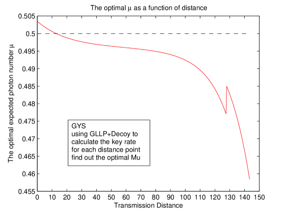
Figure 2: Using numerical analysis to obtain the optimal key generation rate by the formula (11) and use the data GYS in Tab. 1, with parameters listed in Tab. 1.

Now, we would like to do analytical discussion under some approximation. We neglect the dark count, regard $\eta\ll 1$, and consider the ideal error correction efficiency $f(e)=1$. Then (3), (4), (8), (11) will be reduced to,

$$\tilde{p}_{S} \cong p_{S}=\eta\mu e^{-\mu}$$

$$\tilde{\delta}_{S} \cong\delta_{S}=e_{detector}$$

$$p_{D} \cong p_{Signal}=1-e^{-\eta\mu}$$

$$\delta \cong e_{detector}$$

Substitute these formulas into Eq. (11), the key generation rate is given by,

$$R\approx\frac{1}{2}\{-\eta\mu H_{2}(e_{detector})+\eta\mu e^{-\mu}[1-H_{2}(e_{detector})]\}$$

The expression is optimized if we choose $\mu=\mu_{Optimal}$ which fulfills,

$$(1-\mu)\exp(-\mu)=\frac{H_{2}(e_{detector})}{1-H_{2}(e_{detector})}.$$

Then we can solve this equation and obtain that,

$$\mu_{Optimal}^{KTH} \approx 0.8$$

$$\mu_{Optimal}^{GYS} \approx 0.5$$

where for KTH setup $e_{detector}=1\%$, and for GYS $e_{detector}=3.3\%$. Comparing two results we can see that numerical and analytical analysis are compatible.

Chapter 6 Appendix B

In section 3 we use a weak decoy state. Here we would like to discuss how to perform decoy state method in practice.

In decoy method, we require the weak decoy state to be “weak enough” i.e. its expected photon number $\mu\ll 1$. We can then neglect the multi photon term by considering the relationship (7). However, it is not practical for real experiment since it will take a long time to get enough information from weak decoy state if $\mu\ll 1$.

Here we propose one possible solution for weak decoy state, using several (say $m$) weak decoy states with expected photon number $\mu_{1},\mu_{2},\cdot\cdot\cdot\mu_{m}$, instead of one. As discussed in (5), one can estimate the dark count and its error rate accurately. Let us turn our attention to $m$ weak decoy states. With the same argument of (6), we have,

$$p_{D}^{\mu_{j}} =p_{dark}+\sum_{i=1}^{\infty}\eta_{i}\cdot\frac{\mu_{j}^{i}}{i!}\cdot e^{-\mu_{j}}$$ (1)

where $j=1,2,\cdot\cdot\cdot,m$ denotes for the j-th weak decoy state. To solve Eq. (1), we can neglect the high order $(>m)$ terms which are of $O(\mu^{m+1})$, and then Eq. (1) are reduced to,

$$\begin{aligned} p_{D}^{\mu_{1}}&=\sum_{i=0}^{m}\eta_{i}\cdot\frac{\mu_{1}^{i}}{i!}\cdot e^{-\mu_{1}}\\ p_{D}^{\mu_{2}}&=\sum_{i=0}^{m}\eta_{i}\cdot\frac{\mu_{2}^{i}}{i!}\cdot e^{-\mu_{2}}\\ \cdot\cdot\cdot\\ p_{D}^{\mu_{m}}&=\sum_{i=0}^{m}\eta_{i}\cdot\frac{\mu_{m}^{i}}{i!}\cdot e^{-\mu_{m}}\\ \end{aligned}$$ (2)

Now, one can solve $m$ equations for $\{\eta_{i}\}$, $i=1,2,3,\cdot\cdot\cdot,m$. The subsequent procedure is the same as the 3. One can use $\eta=\eta_{1}$ to calculate $\tilde{p}_{S}$ and $\tilde{\delta}_{S}$ by (3) and (4). At last substitute the parameters into (11) to calculate the key generation rate.

How many decoy states should be applied, i.e. $m=?$, depends on how low expected photon number $\mu_{weak}$ one can tolerate. Here, we would like to give out a couple of examples. Given that $\eta=10^{-4}$, suppose that all $m$ decoy states are in the same order. a) If one chooses $\mu_{weak}=O(10^{-3})$ and $m=2$, then the terms neglected are of $O(10^{-9})$ and $p_{S}$ is in the term of $O(\eta\mu)=O(10^{-7})$. Then it is reasonable to neglect the multi photon terms. b) If one chooses $\mu_{weak}=O(10^{-2})$ and $m=3$, then the high order terms neglected are of $O(10^{-8})$ and $p_{S}$ is in the term of $O(\eta\mu)=O(10^{-6})$. Then, one obtains $p_{S}$ and $\delta_{S}$ with precision of around $1\%$.

References

- [1] C. H. Bennett and G. Brassard,“Quantum cryptography: public key distribution and coin tossing”, in Proceedings of IEEE International Conference on Computers, Systems, and Signal Processing, IEEE press, 1984, p. 175.
- [2] A. K. Ekert, “Quantum cryptography based on Bell’s theorem”, Phys. Rev. Lett. vol. 67, p. 661, 1991.
- [3] D. Deutsch, A. Ekert, R. Jozsa, C. Macchiavello, S. Popescu, and A. Sanpera, “Quantum privacy amplification and the security of quantum cryptography over noisy channels”, Phys. Rev. Lett., vol. 77, p. 2818, 1996. Also, [Online] Available: http://xxx.lanl.gov/abs/quant-ph/9604039. Erratum Phys. Rev. Lett. 80, 2022 (1998).
- [4] H.-K. Lo and H. F. Chau, “Unconditional security of quantum key distribution over arbitrarily long distances”, Science 283, 2050-2056 (1999). Also, [Online] Available: http://xxx.lanl.gov/abs/quant-ph/9803006.
- [5] P. W. Shor and J. Preskill, “Simple proof of security of the BB84 quantum key distribution protocol”, Phys. Rev. Lett., vol. 85, p. 441, 2000. Also, [*Online] Available: http://xxx.lanl.gov/abs/quant-ph/0003004.
- [6] W.-Y. Hwang, “Quantum Key Distribution with High Loss: Toward Global Secure Communication”, Phys. Rev. Lett. 91, 057901 (2003)
- [7] Hoi-Kwong Lo, “Quantum Key Distribution with Vacua or Dim Pulses as Decoy States”, unpublished manuscript and presentation at IEEE ISIT 2004.
- [8] D. Gottesman, H.-K. Lo, Norbert Lütkenhaus, and John Preskill,“Security of quantum key distribution with imperfect devices”, quant-ph/0212066 (2004).
- [9] D. Mayers, “Unconditional security in Quantum Cryptography”, Journal of ACM, vol. 48, Issue 3, p. 351-406. Also [Online] Available: http://xxx.lanl.gov/abs/quant-ph/9802025.A preliminary version is D. Mayers, “Quantum key distribution and string oblivious transfer in noisy channels”, Advances in Cryptology-Proceedings of Crypto’ 96 (Springer-Verlag, New York, 1996), p. 343.
- [10] C. Gobby, Z. L. Yuan, and A. J. Shields, “Quantum key distribution over 122 km of standard telecom fiber”, Applied Physics Letters, Volume 84, Issue 19, pp. 3762-3764, (2004)
- [11] M. Koashi, “Unconditional security of coherent-state quantum key distribution with strong phase-reference pulse, ”available on-line at http://xxx.lanl.gov/abs/quant-ph/0403131
- [12] Norbert Lütkenhaus, “Security against individual attacks for realistic quantum key distribution”, quant-ph/9910093 (2004)
- [13] C. H. Bennett, G. Brassard, S. Popescu, B. Schumacher, J. A. Smolin, and W. K. Wootters, “Purification of noisy entanglement and faithful teleportation via noisy channels”, Phys. Rev. Lett. 76, 722-725 (1996), arXiv:quantph/9511027. Erratum: Phys. Rev. Lett. 78, 2031 (1997).
- [14] C. H. Bennett, D. P. DiVincenzo, J. A. Smolin, and W. K. Wootters, “Mixed state entanglement and quantum error correction”, Phys. Rev., vol. A54, 3824, 1996.
- [15] A. R. Calderbank and P. W. Shor, “Good quantum error correcting codes exist”, Phys. Rev. A, vol. 54, pp. 1098 1105, 1996. A. M. Steane, “Multiple particle interference and quantum error correction”, Proc. Roy. Soc. Lond. A, vol. 452, pp. 2551 2577, 1996.
- [16] D. Gottesman and H.-K. Lo, “Proof of security of quantum key distribution with two-way classical communications”, quant-ph/0105121 (2001).
- [17] Muller A, Herzog T, Huttner B, Tittel W, Zbinden H and Gisin N 1997 “Plug&play systems for quantum cryptography”, Appl. Phys. Lett. 70 793-5
- [18] D Stucki, N Gisin, O Guinnard, G Ribordy and H Zbinden, “Quantum key distribution over 67 km with a plug&play system”, New Journal of Physics 4 (2002)
- [19] W. T. Buttler, R. J. Hughes, P. G. Kwiat, G. G. Luther, G. L. Morgan, J. E. Nordholt, C. G. Peterson, and C. M. Simmons, “Free-space quantum key distribution”, quant-ph/9801006 (2004)
- [20] W.T. Buttler, R.J. Hughes, S.K. Lamoreaux, G.L. Morgan, J.E. Nordholt and C.G. Peterson, “Daylight quantum key distribution over 1.6 km”, Phys. Rev. Lett. 84, 24, (2000)
- [21] Kurtsiefer, C.; Zarda, P.; Halder, M.; Weinfurter, H.; Gorman, P. M.; Tapster, P. R.; Rarity, J. G., “A step towards global key distributin”, Nature 419, 450 (2002)
- [22] H.-K. Lo, H. F. Chau, and M. Ardehali, “Efficient Quantum Key Distribution Scheme And Proof of Its Unconditional Security”, available at http://arxiv.org/abs/quant-ph/0011056.
- [23] P. D. Townsend, IEEE Photonics Technology Letters 10, 1048 (1998).
- [24] G. Ribordy, J.-D. Gautier, N. Gisin, O. Guinnard, and H. Zbinden, preprint quant-ph/9905056.
- [25] M. Bourennane, F. Gibson, A. Karlsson, A. Hening, P.Jonsson, T. Tsegaye, D. Ljunggren, and E. Sundberg, Opt. Express 4, 383 (1999).
- [26] G. Brassard and L. Salvail, in Advances in Cryptology EUROCRYPT ’93, Vol. 765 of Lecture Notes in Computer Science, edited by T. Helleseth (Springer, Berlin, 1994), pp. 410-423.
- [27] H. Inamori, N. Lütkenhaus, and D. Mayers, “Unconditional Security of Practical Quantum Key Distribution”, available at http://arxiv.org/abs/quant-ph/0107017
- [28] Kurtsiefer, C.; Zarda, P.; Halder, M.; Weinfurter, H.; Gorman, P. M.; Tapster, P. R.; Rarity, J. G., “A step towards global key distributin”, Nature 419, 450 (2002)
- [29] Hoi-Kwong Lo, Xiongfeng Ma, Kai Chen “Decoy State Quantum Key Distribution”, to be published.