MULTIMODE SQUEEZING PROPERTIES OF A CONFOCAL OPO:
BEYOND THE THIN CRYSTAL APPROXIMATION

Abstract

Up to now, transverse quantum effects (usually labelled as ”quantum imaging” effects) which are generated by nonlinear devices inserted in resonant optical cavities have been calculated using the ”thin crystal approximation”, i.e. taking into account the effect of diffraction only inside the empty part of the cavity, and neglecting its effect in the nonlinear propagation inside the nonlinear crystal. We introduce in the present paper a theoretical method which is not restricted by this approximation. It allows us in particular to treat configurations closer to the actual experimental ones, where the crystal length is comparable to the Rayleigh length of the cavity mode. We use this method in the case of the confocal OPO, where the thin crystal approximation predicts perfect squeezing on any area of the transverse plane, whatever its size and shape. We find that there exists in this case a ”coherence length” which gives the minimum size of a detector on which perfect squeezing can be observed, and which gives therefore a limit to the improvement of optical resolution that can be obtained using such devices.

I Introduction

Nonlinear optical elements inserted in optical cavities have been known for a long time to produce a great variety of interesting physical effects, taking advantage of the field enhancement effect and of the feedback provided by a resonant cavity BoydBob ; Siegman . In particular, a great deal of attention has been devoted to cavity-assisted nonlinear transverse effects, such as pattern formation review1 and spatial soliton generation review2 . More recently the quantum aspects of these phenomena have begun to be studied, mainly at the theoretical level, under the general name of ”quantum imaging”, especially in planar or confocal cavities.

Almost all the investigations relative to intra-cavity nonlinear effects, both at the classical and quantum level, have been performed within the mean field approximation, in which one considers that the different interacting fields undergo only weak changes through their propagation inside the cavity, in terms of their longitudinal and transverse parameters. This almost universal approach simplifies a great deal the theoretical investigations, and numerical simulations are generally needed if one wants to go beyond this approximation Leberre . It implies in particular that diffraction is assumed to be negligible inside the nonlinear medium, which limits the applicability of the method to nonlinear media whose length $l_{c}$ is much smaller than the Rayleigh length $z_{R}$ of the cavity modes $z_{c}$ (so called ”thin” medium). This is a configuration that experimentalists do not like much: they prefer to operate in the case $l_{c}\simeq z_{c}$ which yields a much more efficient non linear interaction for a given pump power boyd . If one wants to predict results of experiments in realistic situations, one therefore needs to extend the theory beyond the usual thin nonlinear medium approximation, and take into account diffraction effects occurring together with the nonlinear interaction inside the medium.

The effects of simultaneous diffraction and nonlinear propagation have already been taken into account in the case of free propagation, i.e. without optical cavity around the nonlinear crystal, and they have been found to have a direct influence on the shape of the propagating beam shen . These effects have also been studied in detail at the quantum level in the parametric amplifier case Brambilla , and recently for the soliton case treps . In contrast, they do not play a significant role when the nonlinear medium is inserted in an optical cavity with non degenerate transverse modes, which imposes the shape of the mode. But they are of paramount importance in the case of cavities having degenerate transverse modes, such as a plane or confocal cavity, which do not impose the transverse structure of the interacting fields, and which are used to generate multimode quantum effects.

Within the thin crystal approximation, i.e. taking into account diffraction effects only outside the crystal, striking quantum properties have been predicted to occur in a degenerate OPO below threshold using a confocal cavity Grangier ; Petsas : this device generates quadrature squeezed light which is multimode in the transverse domain. It was shown in the case of a plane pump that the level of squeezing measured at the output of such an OPO neither depends on the spatial profile of the local oscillator used to probe it, nor on the size of the detection region. This implies that a significant quantum noise reduction, in principle tending to perfection when one approaches the oscillation threshold from below, can be observed in arbitrarily small portions of the down-converted beam. Therefore in this model there is no limitation in the transverse size of the domains in which the quantum noise is reduced when the OPO works in the exact confocal configuration. Such a multimode squeezed light appears thereby as a very promising tool to increase the resolution in optical images beyond the wavelength limit.

It is therefore very important to make a more realistic theoretical model of this system, which is no longer limited by the thin crystal approximation, to see whether the predicted local squeezing is still present in actual experimental realizations in which the crystal length is of the order of the Rayleigh range of the resonator. This is the purpose of the present paper, in which we will show that the presence of a long crystal inside the resonator imposes a lower limit to the size of the regions in which squeezing can be measured (”coherence area”), which is proportional to $w_{c}^{2}l_{c}/z_{R}$, where $w_{c}$ is the cavity beam waist, $l_{c}$ is the crystal length and $z_{R}$ the Rayleigh range of the resonator.

The following section (section II) is devoted to the general description of the model that is used to treat the effect of diffraction inside the crystal, using the assumption that the single pass nonlinear interaction is weak in the crystal. We then describe in section III the method that is used to determine the squeezing spectra measured in well-defined homodyne detection schemes. We give in sections IV and V the results for such quantities respectively in the near field and in the far field, and conclude in section VI.

II The model

II.1 Assumptions of the model

Let us consider a confocal cavity, that for simplicity we take as a ring cavity of the kind shown schematically in Fig. 1 (Schwob Mancini ).

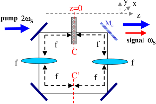
Figure 1: Confocal ring cavity. The mirrors transmit the pump wave and reflect the signal wave, with the exception of mirror $M_{c}$ that partially transmits the signal.

It is formed by four plane mirrors and two lenses having a focal length equal to one quarter of the total cavity length, and symmetrically placed along the cavity, so that the focal points coincides at two positions C and C’. It contains a type I parametric medium of length $l_{c}$, centered on the point C (see figure). It is pumped by a field $A_{p}$ of frequency $2\omega_{s}$ having a Gaussian shape and focused in the plane containing the point C. In such a plane the variation of the mean envelope with the transverse coordinate x is given by :

$$A_{p}(\textbf{x})=A_{p}exp(-\frac{|\textbf{x}|^{2}}{w_{p}^{2}})$$ (1)

We assume that the mirrors are totally transparent for the pump wave, and perfectly reflecting for the field at frequency $\omega_{s}$, except for the coupling mirror $M_{c}$, which has a small transmission $t$ at this frequency. The system was described in Petsas under the thin parametric medium approximation. We will follow here the same approach, generalized to the case of a thick parametric medium of length $l_{c}$. The intracavity signal field at frequency $\omega_{s}$ is described by a field envelope operator $\hat{B}(\textbf{x},z)$, where $z$ is the longitudinal coordinate along the cavity ($z=0$ corresponding to plane C), obeying the standard equal time commutation relation at a given transverse plane at position $z$:

$$[\hat{B}(\textbf{x},z,t),\hat{B}^{\dagger}(\textbf{x'},z,t)]=\delta(\textbf{x}-\textbf{x'}).$$ (2)

As we are only interested in the regime below threshold and without pump depletion, the pump field fluctuations do not play any role.

In a confocal resonator the cavity resonances corresponds to complete sets of Gauss-Laguerre modes with a given parity for transverse coordinate inversion; we assume that a set of cavity even modes is tuned to resonance with the signal field, and that the odd modes are far off-resonance. It is then useful to introduce the even part of the field operator:

$$\hat{B}_{+}(\textbf{x},z,t)=\frac{1}{2}\{\hat{B}(\textbf{x},z,t)+\hat{B}(-\textbf{x},z,t)]\,,$$ (3)

which obeys a modified commutation relation:

$$[\hat{B}_{+}(\textbf{x},z,t),\hat{B}_{+}^{\dagger}(\textbf{x'},z,t)]=\frac{1}{2}[\delta(\textbf{x}-\textbf{x'})+\delta(\textbf{x}+\textbf{x'})]$$ (4)

and can be written as an expansion over the even Gauss-Laguerre modes:

$$\hat{B}_{+}(\textbf{x},z,t)=\sum_{p,leven}f_{p,l}(\textbf{x},z)\hat{a}_{p,l}(z,t)\,,$$ (5)

where $\hat{a}_{p,l}(z,t)$ is the annihilation operator of a photon in mode $(p,l)$ at the cavity position $z$ and at time $t$.

The interaction Hamiltonian of the system in the interaction picture is given by

$$H_{int}=\frac{i\hbar g}{2l_{c}}\int_{-l_{c}/2}^{l_{c}/2}dz^{\prime}\int\int d^{2}x^{\prime}\{A_{P}(\textbf{x'},z^{\prime})[\hat{B_{+}^{\dagger}}(\textbf{x'},z^{\prime},t)]^{2}-h.c.\}\,,$$ (6)

where g is the coupling constant proportional to the second order nonlinear susceptibility $\chi^{(2)}$. This equation generalizes the thin medium parametric Hamiltonian of Ref.GattiLugiato .

II.2 Evolution equation in the image plane (near-field)

In previous approaches Grangier ; Petsas , the crystal was assumed to be thin, so that one could neglect the longitudinal dependence of $A_{P}$ and $\hat{B}_{+}$ along the crystal length in the Hamiltonian (6). This cannot be done in a thick crystal. We will nevertheless make a simplifying assumption which turns out to be very realistic in the c.w. regime, with pump powers below 1W. We assume that the nonlinear interaction is very weak, so that it does not affect much the field amplitudes in a single pass through the crystal. We will therefore remove the $z$ dependence of the operators $\hat{a}_{p,l}$ in Eqs.(5, 6), assuming $\hat{a}_{p,l}(z,t)=\hat{a}_{p,l}(z=0,t)=\hat{a}_{p,l}(t)$, where $z=0$ is the crystal/cavity center C. The longitudinal variation of the signal operator $\hat{B}$ is then only due to diffraction and is described by the well-known $z$ dependence of the modal functions $f_{p,l}(\textbf{x},z)$. This assumption leads to a rather simple expression of the commutator for the $\hat{B}_{+}$ field at different positions inside the crystal:

$$[\hat{B}_{+}(\textbf{x},z,t),\hat{B}_{+}^{\dagger}(\textbf{x'},z^{\prime},t^{\prime})]=G_{+}^{*}(z-z^{\prime};\textbf{x},\textbf{x'})\,.$$ (7)

Here $G_{+}(z;\textbf{x},\textbf{x'})$ is the symmetrized part of the Fresnel propagator $G(z;\textbf{x},\textbf{x'})$, describing the field linear propagation inside the crystal:

$$G_{+}(z;\textbf{x},\textbf{x'})=\frac{1}{2}[G(z;\textbf{x},\textbf{x'})+G(z;\textbf{x},-\textbf{x'})]\,.$$ (8)

with

$$G(z;\textbf{x},\textbf{x'})=\frac{ik_{s}}{2\pi z}e^{ik_{s}\frac{|\textbf{x}-\textbf{x}^{\prime}-\mbox{\boldmath${\rho}$}_{s}z|^{2}}{2z}}\,,$$ (9)

where $k_{s}=n_{s}\omega_{s}/c$ is the field wavenumber, with $n_{s}$ being the index of refraction at frequency $\omega_{s}$, and we have introduced a walk-off term, present only if the signal wave is an extraordinary one, described by the two-dimensional walk-off angle $\mbox{\boldmath${\rho}$}_{s}$.

It is now possible to derive the time evolution of the field operator $\hat{B}(\textbf{x},z,t)$ due to the parametric interaction. We will for example calculate it at the mid-point plane $z=0$ of the crystal :

$$\left.\frac{\partial\hat{B}_{+}}{\partial t}(\textbf{x},0,t)\right|_{int}=g\int\int d^{2}x"K_{int}(\textbf{x},\textbf{x"})\hat{B}_{+}^{\dagger}(\textbf{x"},0,t)$$ (10)

with the integral kernel $K_{int}$ given by :

$$K_{int}(\textbf{x},\textbf{x"}) = \frac{1}{l_{c}}\int_{-l_{c}/2}^{l_{c}/2}dz^{\prime}\int\int d^{2}x^{\prime}$$

$$A_{P}(\textbf{x'},z^{\prime})G_{+}^{*}(z^{\prime};\textbf{x'},\textbf{x})G_{+}^{*}(z^{\prime};\textbf{x'},\textbf{x"})\,.$$

In the limit of a thin crystal considered in Refs.Grangier ; Petsas , Eq. (II.2) is replaced by the simpler expression :

$$\frac{\partial\hat{B}_{+}}{\partial t}(\textbf{x},0,t)|_{int}=gA_{P}(\textbf{x})\hat{B}_{+}^{\dagger}(\textbf{x},0,t)$$ (12)

In the thin crystal case (Eq.(12)), the parametric interaction is local, i.e. the operators at different positions of the transverse plane are not coupled to each other, whereas in the thick crystal case (Eq.(II.2)), the parametric interaction mixes the operators at different points of the transverse plane, over areas of finite extension. Note however that operators corresponding to different $z$ values are not coupled to each other, because of our assumption of weak parametric interaction. This situation is very close to the one considered in refs.Kolobov1 ; Kolobov2 ; Brambilla for parametric down-conversion and amplification in a single-pass crystal, where finite transverse coherence areas for the spatial quantum effects arise because of the finite spatial emission bandwidth of the crystal. In a similar way, in our case the spatial extension of the kernel $K_{int}$ will turn out to give the minimum size in which spatial correlation or local squeezing can be observed in such a system. The analogy will become more evident in the next section, where we will explicitly solve the propagation equation of the Fourier spatial modes along the crystal.

In order to get the complete evolution equation for the signal beam, one must add the free Hamiltonian evolution of the intracavity beam and the damping effects. This part of the treatment is standard Gardiner , and is identical to the case of a thin crystal inserted in a confocal cavity Petsas . The final evolution equation reads:

$$\frac{\partial\hat{B}_{+}}{\partial t}(\textbf{x},0,t)=-\gamma(1+i\Delta)\hat{B}_{+}(\textbf{x},0,t)$$ (13)

$$+g\int\int d^{2}x"K_{int}(\textbf{x},\textbf{x"})\hat{B}_{+}^{\dagger}(\textbf{x"},0,t)+\sqrt{2\gamma}\hat{B}_{+\,in}(\textbf{x},0,t)$$

where $\gamma$ is the cavity escape rate, $\Delta$ the normalized cavity detuning of the even family of modes closest to resonance with the signal field, and $\hat{B}_{in}$ the input field operator.

In order to evaluate the coupling kernel, let us first take into account the diffraction of the pump field, focussed at the center of the crystal, $z=0$. It is described by the Fresnel propagator $G_{p}(z;\textbf{x},\textbf{x'})$, equal to (9) when one replaces $k_{s}$ by the pump wavenumber $k_{p}$, and the signal walk-off angle $\mbox{\boldmath${\rho}$}_{s}$ with the pump walk-off angle $\mbox{\boldmath${\rho}$}_{p}$. One then gets :

$$K_{int}(\textbf{x},\textbf{x"})=\frac{1}{l_{c}}\int_{-l_{c}/2}^{l_{c}/2}dz^{\prime}\int d^{2}x^{\prime}\int d^{2}y$$ (14)

$$A_{p}(\textbf{y})G_{p}(z^{\prime},0;\textbf{x'},\textbf{y})G_{+}^{*}(z^{\prime},0;\textbf{x'},\textbf{x})G_{+}^{*}(z^{\prime},0;\textbf{x'},\textbf{x"})$$

Assuming for simplicity exact collinear phase matching $k_{p}=2k_{s}$, and neglecting the walk-off of the extraordinary wave , four of the five integrations can be exactly performed, and one finally gets:

$$K_{int}(\textbf{x},\textbf{x"}) = \frac{1}{2}\left[A_{p}(\frac{\textbf{x}+\textbf{x"}}{2})\Delta(\textbf{x}-\textbf{x"})\right.$$ (15)

$$\left.+A_{p}(\frac{\textbf{x}-\textbf{x"}}{2})\Delta(\textbf{x}+\textbf{x"})\right]$$

with

$$\Delta(\textbf{x}\pm\textbf{x"})=\frac{ik_{s}}{4\pi l_{c}}\int_{-l_{c}/2}^{l_{c}/2}\frac{dz^{\prime}}{z^{\prime}}e^{\frac{ik_{s}}{4z^{\prime}}|\textbf{x}\pm\textbf{x"}|^{2}}$$ (16)

It can be easily shown that the function $\Delta(\textbf{x}\pm\textbf{x"})$ tends to the usual two-dimensional distribution $\delta(\textbf{x}\pm\textbf{x"})$ when $l_{c}\rightarrow 0$, and that it can be written in terms of the integral sine function $Si(x)=\int_{0}^{x}\frac{sinudu}{u}$ Abramowitz

$$\Delta(\textbf{x}\pm\textbf{x"})=\frac{k_{s}}{2\pi l_{c}}\left(\frac{\pi}{2}-Si(\frac{k_{s}|\textbf{x}\pm\textbf{x"}|^{2}}{2l_{c}})\right)$$ (17)

This expression shows us that $\Delta$ takes negligible values when $|\textbf{x}\pm\textbf{x"}|\gg\sqrt{\frac{\lambda l_{c}}{\pi n_{s}}}$. Fig.2 plots $\Delta$ as a function of the distance $|\textbf{x}\pm\textbf{x"}|$ scaled to

$$l_{coh}=\sqrt{\frac{\lambda l_{c}}{\pi n_{s}}}=w_{C}\sqrt{\frac{l_{c}}{n_{s}z_{C}}}\,,$$ (18)

where $w_{C}$ and $z_{C}$ are the cavity waist and Rayleigh range, respectively.

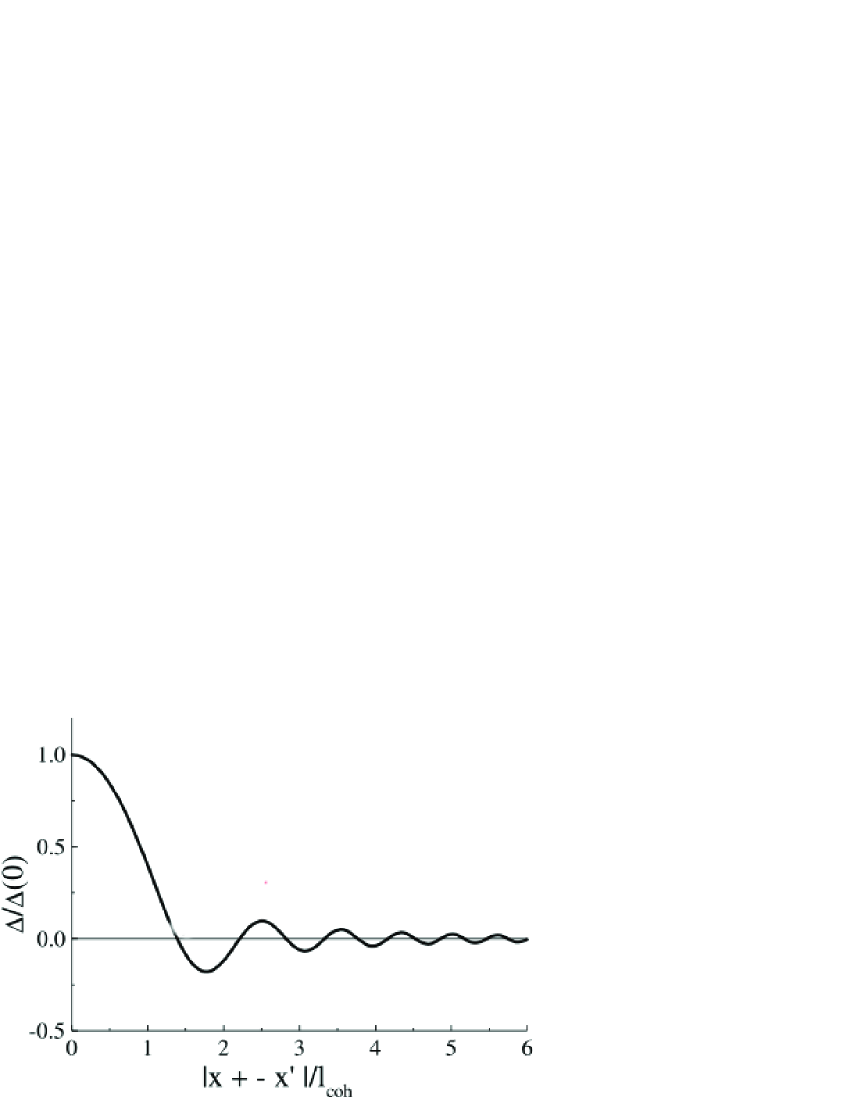
Figure 2: Evaluation of the coupling kernel. $\Delta$ given by Eq. (16) is plotted as a function of $|\textbf{x}\pm\textbf{x"}|$ scaled to the coherence length (18). The first zero of $\Delta$ is obtained for the value $1.37$ of the coordinate.

This expression shows that when the crystal length is on the order of the Rayleigh range of the resonator, the transverse coherence length is on the order of the cavity waist. Recalling that the pump field has a Gaussian shape of waist $w_{p}$, in order to have a multimode operation one must therefore use a defocussed pump, with $w_{p}\gg w_{c}$, or alternatively use a crystal much shorter than the Rayleigh range of the resonator, which is detrimental for the oscillation threshold of the OPO. The relevant scaling parameter of our problem is therefore

$$b=\frac{w_{p}^{2}}{l_{coh}^{2}}=2n_{s}\frac{z_{p}}{l_{c}}\,,$$ (19)

where $z_{p}$ is the Rayleigh or diffraction length of the pump beam. This parameter sets the number of spatial modes that can be independently excited, and it will turn out to give also the number of modes that can be independently squeezed.

II.3 Evolution equation in the spatial Fourier domain (far-field)

In this section we will investigate the intracavity dynamics of the spatial Fourier amplitude of the signal field, which will offer an alternative formulation of the problem. Fourier modes can be observed in the far-field plane with respect to the crystal center C, which in turn can be detected in the focal plane of a lens placed outside the cavity. Let us introduce the spatial Fourier transform of the signal field envelope operator

$$\hat{B}_{+}(\textbf{q},z,t) = \int\frac{d^{2}x}{2\pi}\hat{B}_{+}(\textbf{x},z,t)e^{-i\textbf{q}\cdot\textbf{x}}$$ (20)

$$= \frac{1}{2}\left[\hat{B}(\textbf{q},z,t)+\hat{B}(-\textbf{q},z,t)\right]$$

Equation (II.2) becomes:

$$\frac{\partial\hat{B}_{+}}{\partial t}(\textbf{q},0,t)=-\gamma(1+i\Delta)\hat{B}_{+}(\textbf{q},0,t)+$$ (21)

$$g\int d^{2}q"\tilde{K}_{int}(\textbf{q},\textbf{q"})\hat{B}_{+}^{\dagger}(\textbf{q"},0,t)+\sqrt{2\gamma}\tilde{B}_{+\,in}(\textbf{q},0,t)\,,$$

where the coupling Kernel $\tilde{K}_{int}(\textbf{q},\textbf{q"})$ is the Fourier transform of the kernel (15) with respect to both arguments. Straightforward calculations show that

$$\tilde{K}_{int}(\textbf{q},\textbf{q'}) = \frac{1}{2}\left(\tilde{A_{p}}(\textbf{q}+\textbf{q'}){\rm sinc}[\frac{l_{c}}{2k_{s}}|\frac{\textbf{q}-\textbf{q'}}{2}|^{2}]\right.$$ (22)

$$\left.+\tilde{A_{p}}(\textbf{q}-\textbf{q'}){\rm sinc}[\frac{l_{c}}{2k_{s}}|\frac{\textbf{q}+\textbf{q'}}{2}|^{2}]\right)\,,$$

where $\tilde{A_{p}}$ is the spatial Fourier transform of the Gaussian pump profile (1), i.e. $\tilde{A}_{p}(\textbf{q})=\frac{w_{p}^{2}}{2}A_{p}\exp{(-|\textbf{q}|^{2}\frac{w_{p}^{2}}{4})}$.

The result (22) can be also derived by solving the propagation equation of the pump and signal wave inside a $\chi^{(2)}$ crystal directly in the Fourier domain and in the limit of weak parametric gain. We will follow here the same approach as in Brambilla and GattiStokes , and write the propagation equation in terms of the spatio-temporal Fourier transform field operators $\hat{A}_{j}(\textbf{q},\omega,z)$ of the pump ($j=p$) and signal ($j=s$) waves. Since the cavity linewidth is smaller by several orders of magnitude than the typical frequency bandwidth of the crystal, the cavity filters a very small frequency bandwidth around the carrier frequency $\omega_{s}$ of the signal; moreover, we have assumed that the pump is monochromatic, so that we can safely neglect the frequency argument in the propagation equations, which take the form

$$\frac{\partial\hat{A}_{j}}{\partial z}(\textbf{q},z)=ik_{jz}(\textbf{q})\hat{A}_{j}(\textbf{q},z)+\hat{P}^{NL}_{j}(\textbf{q},z)\,,$$ (23)

where $\hat{P}^{NL}_{j}$ is the nonlinear term, arising from the second order nonlinear susceptibility of the crystal. $k_{jz}(\textbf{q})=\sqrt{k_{j}^{2}-q^{2}}$ is the projection along the z-axis of the wavevector, with $k_{j}=k_{j}(\omega_{j},\textbf{q})$ being the wave-number, which for extraordinary waves depends also on the propagation direction (identified by q). For the pump wave, we assume an intense coherent beam, that we suppose undepleted by the parametric down-conversion process in a single pass through the crystal, so that

$$\hat{A}_{p}(\textbf{q},z)\to\tilde{A}_{p}(\textbf{q},z)=e^{ik_{pz}(\textbf{q})z}A_{p}(\textbf{q},0)\,,$$ (24)

where we take the crystal center as the reference plane $z=0$. For the signal, the propagation equation is more easily solved by setting $\hat{A}_{s}(\textbf{q},z)=\exp{(ik_{sz}(\textbf{q})z})\hat{a}_{s}(\textbf{q},z)$. The evolution along $z$ of the operator $\hat{a}_{s}$ is only due to the parametric interaction and is governed by the equation (see e.g.Brambilla and GattiStokes for more details):

$$\frac{\partial\hat{a}_{s}}{\partial z}(\textbf{q},z)=\frac{\sigma}{l_{c}}\int d^{2}q^{\prime}\,A_{p}(\textbf{q}+\textbf{q}^{\prime},0)\hat{a}_{s}^{\dagger}(\textbf{q}^{\prime},z)e^{i\delta(\textbf{q},\textbf{q}^{\prime})z}\,,$$ (25)

where $\sigma/l_{c}$ is the parametric gain per unit length, and we have introduced the phase mismatch function

$$\delta(\textbf{q},\textbf{q}^{\prime})=k_{pz}(\textbf{q}+\textbf{q}^{\prime})-k_{sz}(\textbf{q})-k_{sz}(\textbf{q}^{\prime}).$$ (26)

Equation (25) has the formal solution

$$\hat{a}_{s}(\textbf{q},\frac{l_{c}}{2}) = \hat{a}_{s}(\textbf{q},-\frac{l_{c}}{2})+\frac{\sigma}{l_{c}}\int_{-\frac{l_{c}}{2}}^{\frac{l_{c}}{2}}dz^{\prime}\int d^{2}q^{\prime}$$ (27)

$$A_{p}(\textbf{q}+\textbf{q}^{\prime},0)\hat{a}_{s}^{\dagger}(\textbf{q}^{\prime},z^{\prime})e^{i\delta(\textbf{q},\textbf{q}^{\prime})z^{\prime}}\,.$$

Assuming a weak parametric efficiency $\sigma\ll 1$, we can solve this equation iteratively. At first order in $\sigma$ the solution reads:

$$\hat{a}_{s}(\textbf{q},\frac{l_{c}}{2})=\hat{a}_{s}(\textbf{q},-\frac{l_{c}}{2})+\sigma\int d^{2}q^{\prime}\,K_{1}(\textbf{q},\textbf{q}^{\prime})\hat{a}_{s}^{\dagger}(\textbf{q}^{\prime},0)\,,$$ (28)

with

$$K_{1}(\textbf{q},\textbf{q}^{\prime})=\tilde{A}_{p}(\textbf{q}+\textbf{q}^{\prime},0)\rm{sinc}{\left[\delta(\textbf{q},\textbf{q}^{\prime})\frac{l_{c}}{2}\right]}\,.$$ (29)

We observe that in the paraxial approximation $k_{jz}(\textbf{q})\approx k_{j}-{\bf\rho}_{j}\cdot\textbf{q}-\frac{q^{2}}{2k_{j}}$, where ${\bf\rho}_{j}$ is the walk-off angle and $k_{j}=n_{j}\omega_{j}/c$. The phase mismatch function is hence given by:

$$\delta(\textbf{q},\textbf{q}^{\prime}) = k_{p}-2k_{s}+({\bf\rho}_{s}-{\bf\rho}_{p})\cdot(\textbf{q}+\textbf{q}^{\prime})$$ (30)

$$-\frac{|\textbf{q}+\textbf{q}^{\prime}|^{2}}{2k_{p}}+\frac{1}{2k_{s}}(q^{2}+q^{\prime 2})$$

Assuming exact phase matching $k_{p}=2k_{s}$, and neglecting the walk-off term, the argument of the sinc function in Eq. (29) becomes

$$\delta(\textbf{q},\textbf{q}^{\prime})\frac{l_{c}}{2}=\frac{l_{c}}{2k_{s}}\left|\frac{\textbf{q}-\textbf{q}^{\prime}}{2}\right|^{2}$$ (31)

In this way we start to recover the result of the Hamiltonian formalism used to derive Eqs.(II.3) and (II.2), where, however, the effect of walk-off and phase mismatch were neglected for simplicity. Indeed, it is not difficult to show that the variation of the intracavity field operator $\hat{B}_{+}(\textbf{q},0,t)$ per cavity round trip time $\tau$, due to the parametric interaction in a single pass through the crystal is

$$\left.\frac{1}{\tau}\Delta\hat{B}_{+}(\textbf{q},0,t)\right|_{int} = \frac{\sigma}{\tau}\int d^{2}q^{\prime}\,\frac{1}{2}\left[K_{1}(\textbf{q},\textbf{q}^{\prime})\right.$$ (32)

$$\left.+K_{1}(\textbf{q},-\textbf{q}^{\prime})\right]\hat{B}_{+}^{\dagger}(\textbf{q}^{\prime},0,t)\,.$$

This approach permits us to understand the physical origin of the sinc terms in the coupling kernel of Eq. (22) (which are the Fourier transform of the $\Delta$ terms in Eq. (15)), that is the limited phase-matching bandwidth of the nonlinear crystal. For a crystal of negligible length, phase matching is irrelevant and there is no limitation in the spatial bandwidth of down-converted modes, whereas for a finite crystal the cone of parametric fluorescence has an aperture limited to a bandwidth of transverse wavevectors $\Delta q\approx 1/l_{coh}\propto 1/\sqrt{\lambda l_{c}}$. As a consequence of the confocal geometry, the cavity ideally transmits all the Fourier modes, so that the only limitation in spatial bandwidth is that arising from phase matching along the crystal.

We notice that if the pump is defocussed enough, the phase-matching limitation results in a limitation of the spot size $\propto 1/l_{coh}$ in the far-field with respect to the cavity center. Inside this spot, modes are coupled because of the finite size of the pump beam (the terms $\propto\tilde{A_{P}}$ in Eq.(22)), inside a region of size $\propto w_{p}^{-1}$. The relevant parameter which sets the number of Fourier modes that can be independently excited is again given by $b=w_{p}^{2}/l_{coh}^{2}$ (see Eq. (19)).

III Homodyne detection and squeezing spectrum

III.1 Homodyne detection scheme in the far field and near field

The method used for measuring the noise-spectrum outside the cavity is a balanced homodyne detection scheme Special . We will use two configurations: the near-field configuration (x-position basis described in II.B) and the far-field configuration (q-vector basis described in II.C). The complete detection scheme in the near-field case is schematically shown in Fig. 3. The two matching lenses of focal length f image the crystal/cavity center plane C onto the detection planes D and D’. The image focal plane F of the first lens coincides with the object focal plane of the second one, and represents the far-field plane with respect to the cavity center C. In planes C,F,D the signal field has its minimum waist, and it has a flat wavefront.

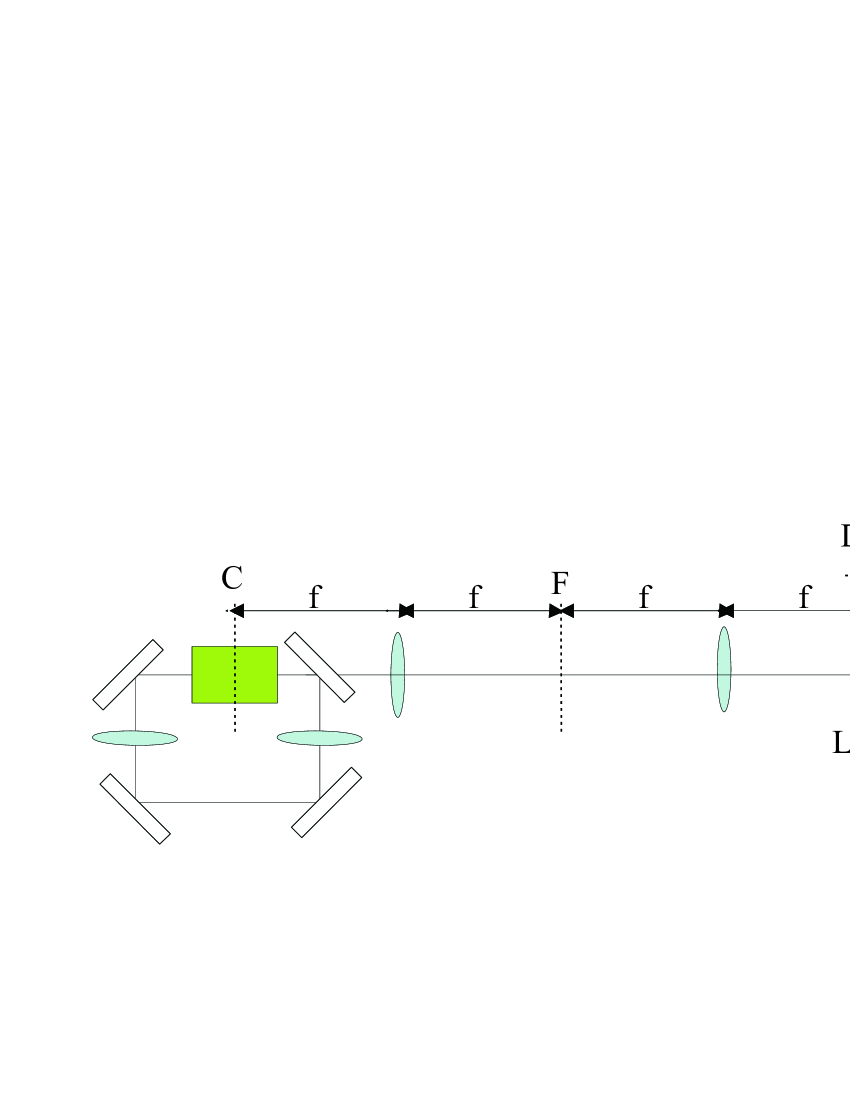
Figure 3: Balanced homodyne detection scheme in the near field. Two matching lenses of focal f are used to image the cavity center C at the detection planes D and D’

The detection scheme in the far field is obtained by using only one lens as depicted in Fig. 4. The focal length f lens is used to image the far field plane with respect of the cavity center C onto the detection plane D.

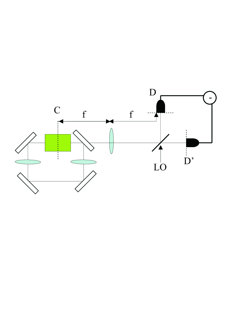
Figure 4: Balanced homodyne detection scheme in the far field. A matching lens of focal f is used to make the far field image of the cavity center C at the detection planes D and D’

The symmetrical beam-splitter BS (reflection and transmission coefficients $\textit{r}=\frac{1}{\sqrt{2}}$ and $\textit{t}=\frac{1}{\sqrt{2}}$) mixes the output signal field with an intense stationary and coherent beam $\alpha_{L}(\textbf{x},z)$, called local oscillator (LO). Note that all the fields being evaluated at the beam-splitter location, we will omit the z-dependence in the following. The difference photocurrent is a measure of the quadrature operator:

$$E_{H}(\Omega)=\int_{det}\!\!\!\!d\textbf{x}\left[B^{out}(\textbf{x},\Omega)\alpha_{L}^{*}(\textbf{x})+B^{out+}(\textbf{x},-\Omega)\alpha_{L}(\textbf{x})\right]\,$$ (33)

where det is the reciprocal image of the photodetection region at the beamsplitter plane, and assumed to be identical for the two photodetectors. We have also assumed here that the quantum efficiency of the photodetector is equal to $1$. Here $B^{out}$ is the sum of its odd and even part:

$$B^{out}(\textbf{x},\Omega)=B^{out}_{+}(\textbf{x},\Omega)+B^{out}_{-}(\textbf{x},\Omega)$$ (34)

The fluctuations $\delta E_{H}(\Omega)$ of the homodyne field around steady state are characterized by a noise spectrum:

$$V(\Omega)=\int_{-\infty}^{+\infty}d\Omega^{\prime}\langle\delta E_{H}(\Omega)\delta E_{H}(\Omega^{\prime})\rangle=N+S(\Omega)$$ (35)

where $E_{H}$ is normalized so that $N$ gives the mean photon number measured by the detector

$$N=\int_{det}dx|\alpha_{L}(x)|^{2}$$ (36)

N represents the shot-noise level, and S is the normally ordered part of the fluctuation spectrum, which accounts for the excess or decrease of noise with respect to the standard quantum level.

III.2 Input/output relation

The relation linking the outgoing fields $B^{out}_{\pm}(\textbf{x},t)$ with the intracavity and input fields at the cavity input/output portGardiner is:

$$B^{out}_{\pm}(\textbf{x},t)=\sqrt{2\gamma}B_{\pm}(\textbf{x},t)-B^{in}_{\pm}(\textbf{x},t)$$ (37)

Equation (13) in the near-field (or (21) in the far field case) is easily solved in the frequency domain, by introducing:

$$B^{in/out}_{\pm}(\textbf{x},\Omega)=\int\frac{dt}{\sqrt{2\pi}}B^{in/out}_{\pm}(\textbf{x},t)e^{-i\Omega t}$$

Taking into account the boundary condition (37), we obtain the input/output relation:

$$[i\Omega+\gamma(1+i\Delta)][B^{out}_{+}(\textbf{x},\Omega)+B^{in}_{+}(\textbf{x},\Omega)] = 2\gamma B^{in}_{+}(\textbf{x},\Omega)+\frac{\gamma}{i\Omega+\gamma(1-i\Delta)}\int\!\!\!\int d^{2}\textbf{x}^{{}^{\prime}}K_{int}(\textbf{x},\textbf{x}^{{}^{\prime}})\Big{[}2\gamma B^{in+}_{+}(\textbf{x}^{{}^{\prime}},-\Omega)$$ (38)

$$+\int\!\!\!\int d^{2}\textbf{x}^{{}^{\prime\prime}}\gamma K_{int}^{*}(\textbf{x}^{{}^{\prime}},\textbf{x}^{{}^{\prime\prime}})(B^{in}_{+}(\textbf{x}^{{}^{\prime\prime}},\Omega)+B^{out}_{+}(\textbf{x}^{{}^{\prime\prime}},\Omega))\Big{]}$$

In the case of a thin crystal in the near fieldPetsas or a plane pump in the far field, this relation describes an infinite set of independent optical parametric oscillators. In these cases the squeezing spectrum can be calculated analytically as we will see in the following. But in other cases, this relation links all points in the transverse plane. In order to get the input/output relation, we have to inverse relation (38) by using a numerical method.

III.3 Numerical method

In order to inverse relation (38) by numerical means, we need to discretise the transverse plane in order to replace integrals by discrete sums. For the sake of simplicity, we will only describe here the solution in the single transverse dimension model: the cavity is assumed to consist of cylindrical mirrors, so that the the transverse fields depend on a single parameter, y. In this case the electromagnetic fields are represented by vectors and the interaction terms by matrices. Straightforward calculations show that we can introduce the interaction functions $U(y,y^{\prime})$ and $V(y,y^{\prime})$ (calculated at resonance $\Delta=0$ and at zero frequency in near-field or far-field configurations ) linking two different points in the transverse plane, so that relation (38) becomes:

$$B_{+}^{out}(y) = \int_{-\infty}^{\infty}dy^{\prime}U(y,y^{\prime})B_{+}^{in}(y^{\prime})$$ (39)

$$+\int_{-\infty}^{\infty}dy^{\prime}V(y,y^{\prime})B_{+}^{in+}(y^{\prime})$$

Since we assumed that the odd part of the output field is in the vacuum state, $B_{-}^{out}$ gives no contribution to the normally ordered part of the spectrum $S$, which can be calculated by using the input/output relation (21) for the even part of the field, and by using the commutation rules for the even part:

$$[B^{in/out}_{\pm}(x,t),B^{in/out+}_{\pm}(x^{\prime},t^{\prime})]=$$

$$\frac{1}{2}[\delta(x-x^{\prime})\pm\delta(x+x^{\prime})]\delta(t-t^{\prime})$$ (40)

In the following, we will assume, as in Refs.Petsas Grangier , that the local oscillator has a constant phase profile $\varphi_{L}(\textbf{x})=\varphi_{L}$, so that $\alpha_{L}(x)=|\alpha_{L}(x)|e^{i\varphi_{L}}$. We obtain the ordered part of the spectrum, normalized to the shot noise:

$$\frac{S(0)}{N}=\frac{1}{\int_{det}dy|\alpha_{L}|^{2}}\int\int_{det^{2}}dxdx^{\prime}\int_{-\infty}^{+\infty}dy|\alpha_{L}(x)||\alpha_{L}(x^{\prime})| \Big{[}(V(x,y)V(x^{\prime},y)+V(x,y)V(x,-y))$$ (41)

$$+\cos(2\varphi_{L})(U(x,y)V(x^{\prime},y)+U(x,y)V(x^{\prime},-y))\Big{]}$$

Now, knowing the $U(y,y^{\prime})$ and $V(y,y^{\prime})$ interaction functions, we are able to calculate the squeezing spectrum in both near and far-field cases.

IV Squeezing spectrum in the near-field

In this section, we use the near-field homodyne detection (Fig. 3) described in Ref.Petsas . As already said in part II, in the near field, the thick crystal couples pixels contained in a region whose size is in the order of $l_{coh}$ (18).

Let us study first the case of a plane-wave pump and a plane-wave local oscillator. As pointed out in refGrangier , in this case and in the thin crystal approximation, the level of squeezing does not depend on the width of the detection region. Fig. 5 shows results predicted for a measurement performed with a circular detector of radius $\triangle\rho$ centered on the cavity axis (which is a symmetric detection area, as pointed out in Petsas ). We represent the squeezing spectrum at zero frequency as a function of the size of the detector, scaled to the coherence length $l_{coh}=\sqrt{\frac{\lambda l_{c}}{\pi n_{s}}}$. We can see that for $\Delta\rho<l_{c}$, the squeezing tends to zero when $\Delta\rho\longrightarrow 0$, as already predicted. For larger values of the detector size, perfect squeezing can be achieved. We can also see that the squeezing evolution is comparable to the $\triangle$ function evolution (Fig. 2).

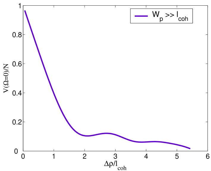
Figure 5: Squeezing spectrum at zero-frequency, normalized to the shot noise, as a function of the detector radius (scaled to $l_{coh}$).

In the more realistic case of finite size pump, the squeezing level depends on the parameter $b=\frac{w_{p}^{2}}{l_{coh}^{2}}=2n_{s}\frac{z_{p}}{l_{c}}$, as pointed out in part I. Fig. 6 represents the squeezing spectrum at zero-frequency as a function the detector radius, normalized to $l_{coh}$, for different b parameters, using a plane local oscillator. As already seen in Fig. 5, for $\Delta\rho\longrightarrow 0$, the noise reduction effect tends to zero. But we see now that there is also no squeezing effect for large values of the detector radius, because of the finite size of the pump, as already shown in Petsas .

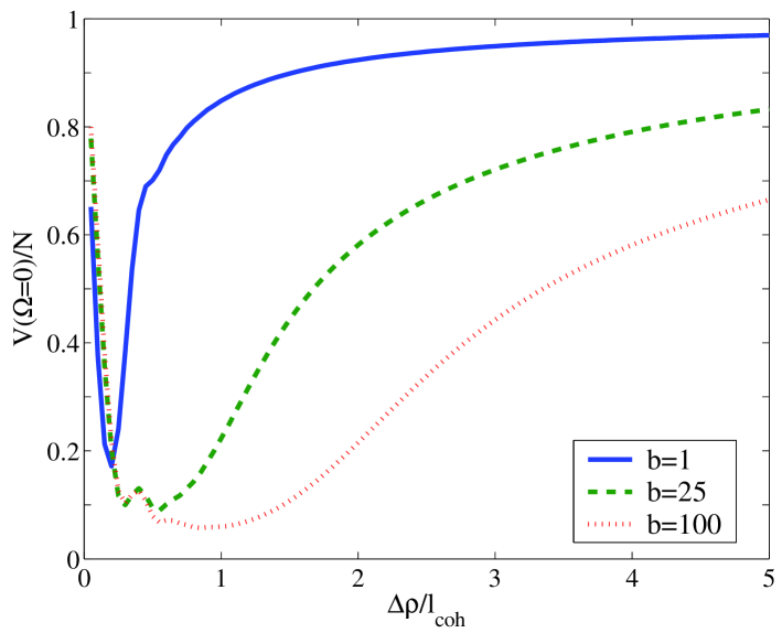
Figure 6: Squeezing spectrum at zero-frequency, normalised to the shot noise, as a function of the radial amplitude of the detector scaled to $l_{coh}$, plotted for several values of b

Fig. 7 shows theoretical results in the case of a detector consisting of two symmetric pixels (pixel of size equal to the coherence length), for different b values, in function of the distance between the two pixels.

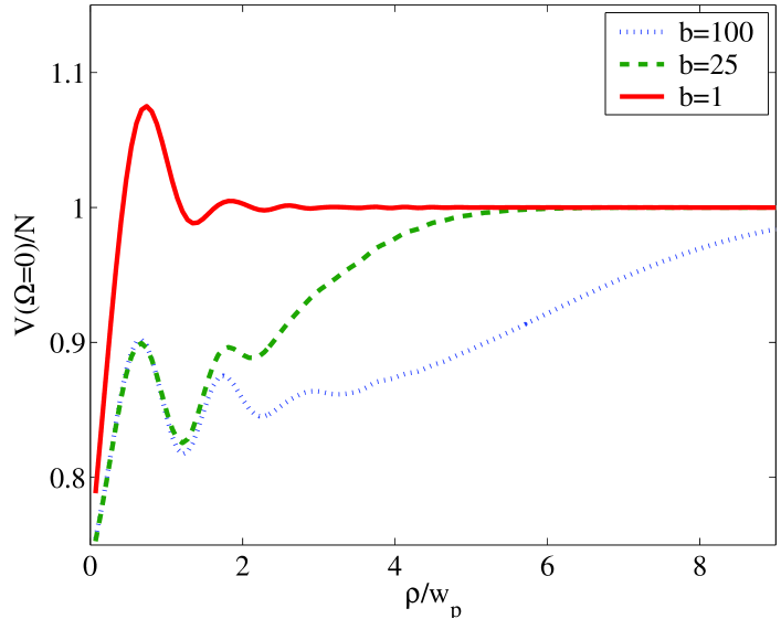
Figure 7: Squeezing spectrum at zero-frequency, normalised to the shot noise, as a function of the pixel distance between the two pixels $\rho$ from the cavity axis (scaled to $l_{coh}$), plotted for several values of b

For large values of $\rho$, the noise level goes back to shot noise because of the finite size of the pump, as already depicted in reference Petsas . But now, for small $\rho$ values, the squeezing does not tend to zero, as in the thin crystal case.

V Squeezing spectrum in the far-field

In this section, we will consider the spatial squeezing spectrum in the far field (Fig. 4) and in the q-vector basis. As already said in section II.C, the coupling between q-vectors modes is now due to the finite length of the pump. We will see that a new coherence length $l_{cohf}$ appears in such a case, given by:

$$l_{cohf}\propto\frac{1}{w_{p}}$$

. We will successively investigate two configurations: the plane wave pump regime (where the squeezing spectrum can be calculated analytically), and the case of a finite pump size (where a numerical method is necessary).

V.1 Plane wave pump regime in the far field

In order to evaluate the far field case, we introduce the spatial Fourier transforms of the electromagnetic field temporal frequency components:

$$\tilde{B}^{in/out}_{\pm}(\textbf{q},\Omega)=\int\int\frac{d^{2}x}{2\pi}\hat{B}^{in/out}_{\pm}(\textbf{x},\Omega)e^{-i\textbf{q}.\textbf{x}}$$

In the case of a plane wave pump, $A_{p}(\textbf{x},z)=A_{p}$, so that equation(22) becomes:

$$\frac{\partial\tilde{B}_{+}}{\partial t}(\textbf{q},0,t) = -\gamma[(1+i\Delta)\tilde{B}_{+}(\textbf{q},0,t)+\sqrt{2\gamma}\tilde{B}_{+\,in}(\textbf{q},0,t)$$ (42)

$$-A_{p}sinc(\frac{l_{c}\textbf{q}^{2}}{2k_{s}})\tilde{B}_{+}^{\dagger}(\textbf{q},0,t)]$$

This equation, which does not mix different q values, can be solved analytically. It is similar to equation (14) in reference Petsas . Taking into account the boundary condition

$$\tilde{B}^{out}_{\pm}(\textbf{q},t)=\sqrt{2\gamma}\tilde{B}_{\pm}(\textbf{q},t)-\tilde{B}^{in}_{\pm}(\textbf{q},t)$$ (43)

We obtain:

$$\tilde{B}^{out}_{+}(\textbf{q},\Omega)=\textit{U}(\textbf{q},\Omega)\tilde{B}^{in}_{+}(\textbf{q},\Omega)+\textit{V}(\textbf{q},\Omega)\tilde{B}^{in+}_{+}(-\textbf{q},-\Omega)$$ (44)

where

$$\textit{U}(\textbf{q},\Omega)=\frac{[1-i(\Delta-\Omega/\gamma)][1-i(\Delta+\Omega/\gamma)]+A_{p}^{2}sinc^{2}(\frac{l_{c}\textbf{q}^{2}}{2k_{s}})}{[1+i(\Delta+\Omega/\gamma)][1-i(\Delta-\Omega/\gamma)]-A_{p}^{2}sinc^{2}(\frac{l_{c}\textbf{q}^{2}}{2k_{s}})}$$ (45)

and

$$\textit{V}(\textbf{q},\Omega)=$$ (46)

$$\frac{2A_{p}sinc(\frac{l_{c}\textbf{q}^{2}}{2k_{s}})}{[1+i(\Delta+\Omega/\gamma)][1-i(\Delta-\Omega/\gamma)]-A_{p}^{2}sinc^{2}(\frac{l_{c}\textbf{q}^{2}}{2k_{s}})}$$

In the case of plane wave regime, the input/output relation in the spatial Fourier space describes therefore an infinite set of independent optical parametric oscillators below threshold. This can be simply understood: the q-vector basis is the eigenbasis of the diffraction, so that no coupling between q-vector modes due to the crystal appears.

Let us now consider the homodyne-detection scheme, schematically shown in (Fig. 4). The lens provides a spatial Fourier transform of the output field $B_{out}(x,\Omega)$, so that at the location of plane D the field $B_{out}^{D}(x,\Omega)$ is:

$$B_{out}^{D}(x,\Omega)=\frac{2\pi}{\lambda f}\tilde{B}_{out}(\frac{2\pi}{\lambda f}x,\Omega)$$ (47)

In this plane,$B_{out}^{D}(x,\Omega)$ is mixed with an intense stationary and coherent beam $\alpha_{LO}^{D}(x)=\frac{2\pi}{\lambda f}\tilde{\alpha}_{LO}(\frac{2\pi x}{\lambda f},\Omega)$, where $\alpha_{L}(x)$ has a gaussian shape, with a waist $w_{LO}$. The homodyne field has thus an expression similar to the near field case, where functions of $x$ are now replaced by their spatial Fourier transforms:

$$E_{H}(\Omega)=$$ (48)

$$\int_{det}d\textbf{q}[\tilde{B}^{out}(\textbf{q},\Omega)\tilde{\alpha}_{LO}^{*}(\textbf{q})+\tilde{B}^{out+}(\textbf{q},-\Omega)\tilde{\alpha}_{LO}(\textbf{q})]$$

This analogy shows that, in the case of a local oscillator that has an even parity with respect to coordinate inversion, the squeezing spectrum is given by (like in Petsas ):

$$V(\Omega) = \int_{det}d\textbf{q}\{|\tilde{\alpha}_{LO}(\textbf{q})|^{2}[1-\sigma(\textbf{q})]\}$$ (49)

$$+\int_{det}d\textbf{q}\{|\tilde{\alpha}_{LO}(\textbf{q})|^{2}\sigma(\textbf{q})R(\textbf{q},\Omega)\}$$

where the noise spatial density $R(\textbf{q},\Omega)$ is given by:

$$R(\textbf{q},\Omega)=|\textit{U}(\textbf{q},\Omega)+e^{2i\varphi_{LO}(\textbf{q})}\textit{V}^{*}(\textbf{q},-\Omega)|^{2}$$ (50)

and where

$$\sigma(\textbf{q})=\int_{det}d\textbf{q'}\delta_{+}(\textbf{q},\textbf{q'})$$ (51)

In order to minimize $R(\textbf{q},\Omega)$, the local oscillator phase should be chosen as $\varphi_{LO}(\textbf{q})=\frac{arg[U(\textbf{q},\Omega)V(\textbf{q},\Omega)]}{2}$. In particular, at resonance and at zero frequency $U(\textbf{q},0)$ and $V(\textbf{q},0)$ are real and the optimal local oscillator phase would correspond to $\varphi_{LO}(\textbf{q})=\frac{\pi}{2}$, when $sinc(\frac{l_{c}\textbf{q}^{2}}{2k_{s}})\geq 0$, and $\varphi_{LO}(\textbf{q})=0$, when $sinc(\frac{l_{c}\textbf{q}^{2}}{2k_{s}})\leq 0$, which is not indeed very practical. However, modes for which $sinc(\frac{l_{c}\textbf{q}^{2}}{2k_{s}})\leq 0$ are quite outside the phase matching curve, so that the choice $\varphi_{LO}(\textbf{q})=\frac{\pi}{2}$ everywhere should give good results. The squeezing spectrum at resonance and zero frequency, for $\varphi_{LO}(\textbf{q})=\frac{\pi}{2}$ can be analytically calculated and, as a function of the radius $r$ of a detector centered on the optical axis is given by:

$$\frac{V(r,0)}{N} = \frac{1}{\int_{0}^{r/r_{0}}u\exp(\frac{-w_{LO}^{2}k_{s}u^{2}}{l_{c}})}$$

$$*\int_{0}^{r/r_{o}}\!\!\!\!\!u\exp\left(\frac{-w_{LO}^{2}k_{s}u^{2}}{l_{c}}\right)\left(\frac{1+A_{p}sinc(u^{2})}{1-A_{p}sinc(u^{2})}\right)^{2}$$

where

$$r_{0}=\frac{\lambda f}{2\pi}\sqrt{\frac{2k_{s}}{l_{c}}}=\frac{\lambda f}{\pi}*\frac{1}{l_{coh}}$$ (53)

Fig. 8 shows the results obtained in the case of two different detection configurations: the $V$ curve shows results in the case of a circular detector of variable radius $r$ (scaled to $r_{0}$), using a local oscillator waist $w_{LO}=r_{0}$. As already said in part $II$, the limitation of the squeezing level is due to the non perfect phase matching along the crystal. For $r>r_{0}$, the squeezing level decreases. So, in the plane wave pump regime in the far field, the thickness of the crystal has a role comparable with the finite size of the pump in the near field, as reported in Petsas . The $R$ curve shows results obtained in the case of two small symmetrical pixels and a plane wave local oscillator as a function of the pixel distance from the cavity axis $r$, scaled to $r_{0}$. We can see that the noise level goes back to the shot noise level for $r>r_{0}$, because to the non perfect phase matching along the crystal.

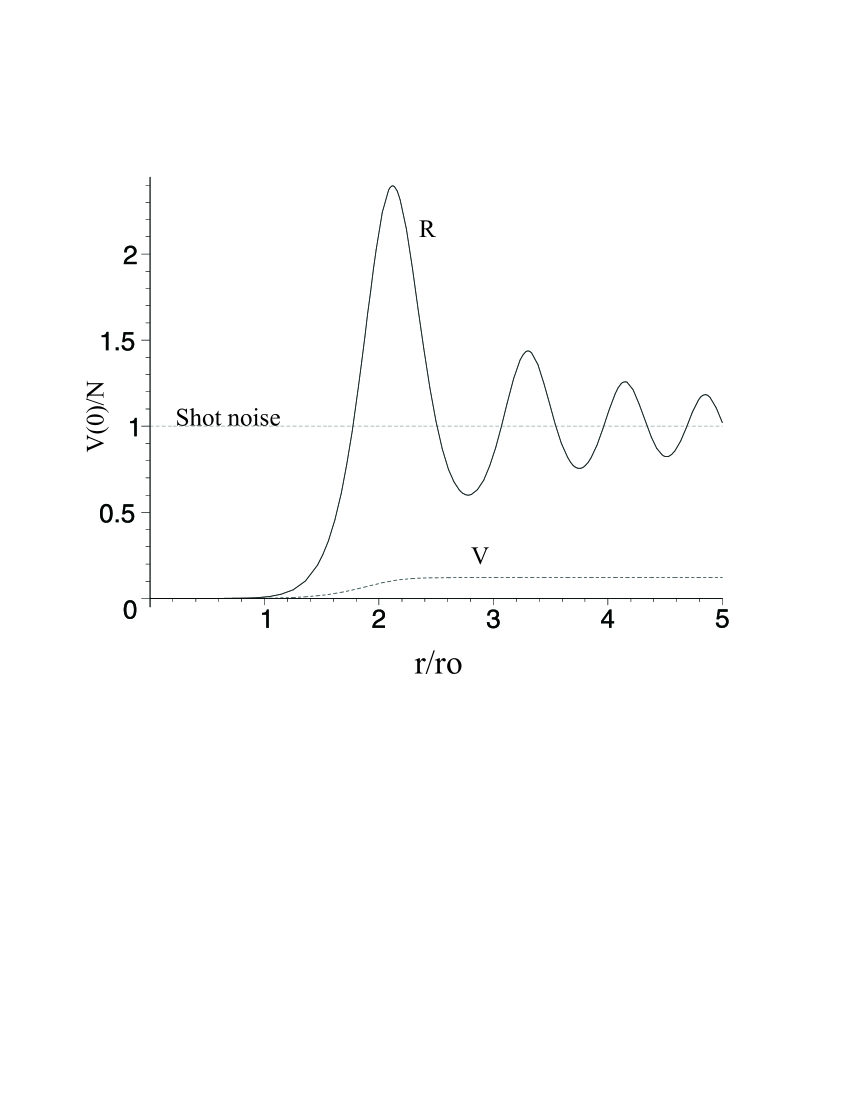
Figure 8: Squeezing spectrum normalized to the shot noise,at zero-frequency, at resonance, in the plane pump regime and far field case, for two measurement configurations. $V$ is obtained using a circular detector of radial amplitude r (scaled to $r_{0}$). $R$ is obtained using a pair of symmetrical pixels in function of the pixel distance from the axis r (scaled to $r_{0}$)

V.2 Squeezing spectrum in the far field case and finite size pump regime

When one takes into account the finite size of the pump, a coupling between different q vectors appear, and one needs to solve equations numerically, as in the near field case. A new coherence length $l_{cohf}$ appears in the far field: $l_{cohf}=\frac{1}{w_{P}}$.

Fig. 9 shows the evolution of the squeezing spectrum at zero frequency, and at resonance, for different b parameters, in function of the detector radius scaled to $l_{cohf}$ . We see the same evolution as in the analytical case, except that the noise level tends to shot noise for small values of the detector.

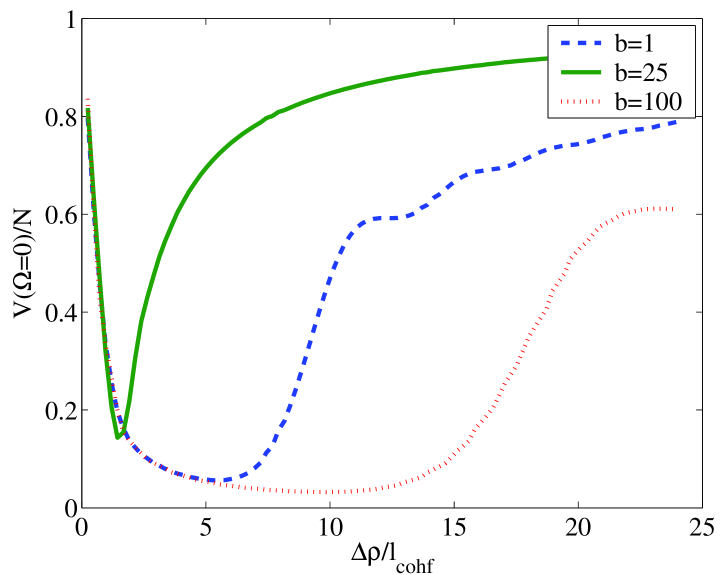
Figure 9: Squeezing spectrum normalized to the shot noise at zero-frequency, and at resonance, as a function of the radial amplitude of the detector $\Delta\rho$(scaled to the coherence area $l_{cohf}$), in the finite pump regime and far field approach and for different values of b.

Fig. 10 shows the results obtained in the case of two symmetrical pixels (pixel of size equal to the coherence length $l_{cohf}$), for different b values, in function of the distance between the two pixels $\rho$. The evolution is similar to the one given by fig(6) for large distances. But there is here also a decrease of the squeezing effect for small distances.

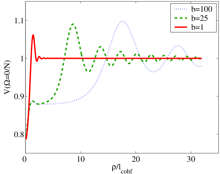
Figure 10: Squeezing spectrum normalized to the shot noise at zero-frequency, and at resonance, as a function of the distance between the two pixels $\rho$ (scaled to the coherence area $l_{cohf}$), in the finite pump regime and far field approach and for different values of b.

VI Discussions and Conclusions

We have seen that when one takes into account the effect of diffraction inside the nonlinear crystal in a confocal OPO, the local squeezing predicted for any shape and size of the detectors in the thin crystal approximation is now restricted to detection areas lying within a given range, characterized by a coherence length $l_{coh}$. This prediction introduces serious limitations to the success of an experiment, and must be taken into account when designing the experimental set-up. With the purpose of producing a light beam that is squeezed in several elementary portions of its transverse cross-section, either a crystal short compared to $z_{R}$ should be used or, alternatively, a defocussed pump, with a waist much larger than the cavity waist. In both cases the efficiency of the non linear coupling is reduced. For instance, with $1cm$ long crystal, $l_{coh}$ is equal to $40\mu m$, and one must choose a pump waist much larger than this value in order to observe multimode squeezing (the number of modes being roughly equal to the ratio $b=\frac{w_{p}^{2}}{l_{coh}^{2}}$). This defocussed pump will imply a much higher threshold for the OPO oscillation, which is multiplied by a factor also close to $b$. The conclusion of this analysis is that one cannot have multimode squeezing ”for free”, and that with a given pump power, one will be able to to excite a number of modes which is roughly equal to the ration of the injected pump power to the threshold power for single mode operation.

References

- (1) W.Boyd, Nonlinear Optics, Academic Press (1992).
- (2) A. Siegman, Lasers, University Science Books.
- (3) Y.R.Shen, The Principles of Nonlinear optics, Wiley Classics Library.
- (4) L.A Lugiato, M Brambilla, A Gatti, Advances in Atomic Molecular and Optical Physics 40, 229 (1998).
- (5) S.Barland, J.R.Tredicce, M.Brambilla, L.A.Lugiato, S.Balle, M.Giudici, T.Maggipinto, L.Spinelli , G.Tissoni, T.Koedl, M.Miller and R.Jaeger, Nature 419, 699 (2002).
- (6) M.I.Kolobov,I.V.Sokolov, Sov.Phys.JETP 69, 1097 (1989).
- (7) M.I.Kolobov, Rev.Mod.Phys 71, 5 (1999).
- (8) E.Brambilla, A.Gatti, M.Bache and L.A.Lugiato, Phys.Rev.A 69, 023802 (2004).
- (9) M. LeBerre, D. Leduc, E. Ressayre, and A. Tallet, J. Opt. B: Quantum Semiclass. Opt. 1, 153 (1999).
- (10) G.Boyd, D.Kleinman, J.Applied Physics 39, 3597 (1968).
- (11) E.Lantz, T.Sylvestre, H.Maillotte, N.Treps, C.Fabre, J. Opt. B: Quantum Semiclass. Opt. 6 S295-S302, (2004).
- (12) L.A.Lugiato, Ph.Grangier, J.Opt.Soc.Am.B 31, 3761 (1985).
- (13) K.I.Petsas,A.Gatti,L.A.Lugiato, and C.Fabre, EPJD 2,125(2002).
- (14) C.Schwob, P.F.Cohadon, C.Fabre, M.A.Marte, H.Ritsch, A.Gatti, L.Lugiato, Applied.Phys.B 66, 685 (1998).
- (15) S.Mancini, A.Gatti, L.Lugiato, Eur.Phys.J.D 12, 499-508 (2000).
- (16) A.Gatti, L.Lugiato, Phys.Rev.A 52, 1675 (1995).
- (17) C.W.Gardiner, M.J.Collet,Phys.Rev.A 31, 3761 (1985).
- (18) Abramowitz and Stegun, Handbook of mathematical functions.
- (19) A.Gatti, R.Zambrini, M.San Miguel, Multiphoton, multimode polarization entanglement in parametric downconversion, Phys. Rev. A 68, 053807 (2003).
- (20) Special issue on Squeezed light, edited by R.Loudon, P.L.Knigth, in J.Mod.Opt 34,(6/7)(1987).