Effective squeezing enhancement via measurement-induced non-Gaussian operation and its application to dense coding scheme

Abstract

We study the measurement-induced non-Gaussian operation on the single- and two-mode Gaussian squeezed vacuum states with beam splitters and on-off type photon detectors, with which mixed non-Gaussian states are generally obtained in the conditional process. It is known that the entanglement can be enhanced via this non-Gaussian operation on the two-mode squeezed vacuum state. We show that, in the range of practical squeezing parameters, the conditional outputs are still close to Gaussian states, but their second order variances of quantum fluctuations and correlations are effectively suppressed and enhanced, respectively. To investigate an operational meaning of these states, especially entangled states, we also evaluate the quantum dense coding scheme from the viewpoint of the mutual information, and we show that non-Gaussian entangled state can be advantageous compared with the original two-mode squeezed state.

I Introduction

Non-classical optical Gaussian states, such as single- or two-mode squeezed vacuum states, play essential roles in continuous variable (CV) quantum information technology. These states have already been implemented in labs and manipulating these states with linear operations including beam splitters, phase shifters, displacements, and homodyne measurements, various quantum information protocols have been demonstrated: teleportation Furusawa98 , dense coding Mizuno05 , and entanglement swapping Jia04 . Mathematically, the operations by these linear optics tools and arbitrary squeezing operations are described by linear and bilinear Hamiltonians and classified as Gaussian operations which transform Gaussian states into Gaussian states.

A class of Gaussian operation is, however, obviously a part of the class of universal quantum operations. Recent theoretical investigation has shown the limitation of Gaussian operations in quantum information processing, e.g. entanglement distillation of Gaussian input to Gaussian output is impossible Eisert02 ; Fiurasek02 ; Giedke02 and, more generally, quantum information protocols consisting of only Gaussian operations can be simulated classically Bartlett02PRL . Therefore, implementation of non-Gaussian operation, that is the operations accessible to the outside of the Gaussian domain, would be crucial to extract ultimate potential of quantum information theory. In addition, a delightful theoretical result is that, in principle, arbitrary operations can be implemented by combining one of non-Gaussian operations with suitable Gaussian operations Lloyd99 ; Bartlett02PRA .

Although, at present, even the cubic nonlinearity is hard to realize on the level of single photon, there is an alternative idea, called the measurement-induced nonlinearity, where effective nonlinearity is associated with non-Gaussian measurement such as photon counting Bartlett02PRA . A simplest example of such operations has been theoretically investigated, where photons in non-classical Gaussian states are subtracted by low reflectance beam splitters and photon counters. It was proposed that one can generate Schrödinger cat-like state from a single-mode squeezed vacuum by subtracting photons Dakna97 . Recently, nonclassicality of this cat-like state has been investigated with respect to negativity of Wigner function, in consideration of some experimental parameters Kim05 .

Moreover, it is predicted that the photon subtraction from two-mode squeezed vacuum can increase entanglement Opatrny00 ; Cochrane02 ; Browne03 . In ideal situation, i.e. perfect photon number counting and lossless setup, the output is always pure and one can uniquely quantify the increase of entanglement by the von Neumann entropy of a partial system. In practical situation, however, imperfections should be taken into account. The main one is the imperfection of photon detector. It is still difficult to distinguish the photon number precisely. Currently available type of detector is the on-off type detector (e.g. avalanche photodiodes in Geiger mode operation) which discriminate only between the vacuum and the presence of photons with finite quantum efficiency and nonzero dark counts. This type of detector suffices for some purposes. In fact, the first observation of non-Gaussian statistics due to the photon subtraction from a single-mode squeezed vacuum was demonstrated using such a type of device Wenger04 .

A serious restriction due to the on-off type resolution is that the detector projects the original state into a mixed state. For instance, in the case where one of the two mode entangled state is measured by the on-off detector, the state of the other mode is projected into a mixed state. Similarly, the photon subtraction with on-off detector reduces the pure two-mode squeezed state to the mixed state. One cannot, therefore, apply the von Neumann entropy to quantify their entanglement. In this direction, some operational measures have been exploited theoretically to characterize the non-Gaussian mixed entangled state. They are, for example, the improvement of the teleportation fidelity Olivares03 and the non-locality due to the violation of Bell type inequality Nha04 ; Garcia-Patron04PRL ; Garcia-Patron04 ; Olivares04 .

In this paper, we consider the photon subtraction scheme consisting of two on-off detectors. The scheme is applied to both single- and two-mode squeezed vacua including realistic parameters of possible imperfections. Special attention is paid to that the density operators conditioned by the on-off detector can be represented in terms of the sum of the three kinds of Gaussian states. Therefore photon subtracted non-Gaussian states may still include Gaussian nature more or less.

Based on this, we address the following two points. First, we discuss the validity of the second order variance as a measure of the performance of the photon subtracted state. Experimentally, the evaluation of the states by the second order variance of quantum fluctuations or correlations are easier and more accurate than the evaluation based on full reconstruction of the states such as quantum tomography. When two on-off detectors are applied to a single-mode squeezed vacuum, one can conditionally generate a plus-cat-like state which is often squeezed than the input. It is shown that in realistic squeezing regime, the squeezing of the photon subtracted state is higher than that of the input. We also show that photon subtractions from two-mode squeezed vacuum greatly enhance the second order quantum correlation of the output in practical parameter regime.

Second, we apply the photon subtracted entangled state to quantum dense coding Ban99 ; Braunstein00 . This is an entanglement-assisted coding to transmit classical information which can attain a larger capacity than that without entanglement Ralph02 . Therefore the increase of the capacity, more precisely, the mutual information for a specified measurement (e.g. the Bell measurement), can be an alternative operational measure for the photon subtracted entangled state. The mutual information is calculated by determining the channel matrix between the input signals and the measurement outcomes. This measure can be a stringent figure of merit for the system in the sense that the gain usually vanishes even with relatively small imperfections. This also specifies the asymptotic rate of transmission when the multiple use of the channels is considered. So it would be worth considering such kind of information theoretic measure to quantify the non-Gaussian state.

This paper is organized as follows: In Sec. II, we discuss the measurement-induced non-Gaussian operation on single-mode squeezed vacuum state, and its equivalence to Schrödinger cat-like state generation in Ref. Dakna97 . In Sec. III, we discuss the two-mode case. The generated non-Gaussian entangled state is applied to the dense coding scheme in Sec. IV. In the Secs. V, VI, and VII, we give analyses with consideration of practical parameters of imperfections. The last section VIII is devoted to discussion and conclusion.

II Non-Gaussian operation on single-mode squeezed vacuum state

We first consider the non-Gaussian operation on the single-mode squeezed vacuum state in the ideal situation. The schematic is shown in Fig. 1. The target mode is denoted by path A. For the later extension to the two mode case, we consider another mode B whose initial state is the vacuum state. The initial state of mode A is the squeezed vacuum state

$$|r\rangle_{k}=\hat{S}_{k}(r)|0\rangle,$$ (1)

where $\hat{S}_{k}(r)$ is the squeezing operator of mode $k$,

$$\hat{S}_{k}(r)=\exp\left[-\frac{r}{2}(\hat{a}_{k}^{\dagger 2}-\hat{a}_{k}^{2})\right],$$ (2)

and $r$ is the squeezing parameter, proportional to the second-order susceptibility and the thickness of the nonlinear optical crystal and the pump intensity. For this state, the uncertainty is reduced in terms of the $x-$ quadrature corresponding to $\varphi=0$ in the following quadrature operator

$$\hat{x}_{\varphi}=\frac{1}{\sqrt{2}}\left(\hat{a}e^{-i\varphi}+\hat{a}^{\dagger}e^{i\varphi}\right).$$ (3)

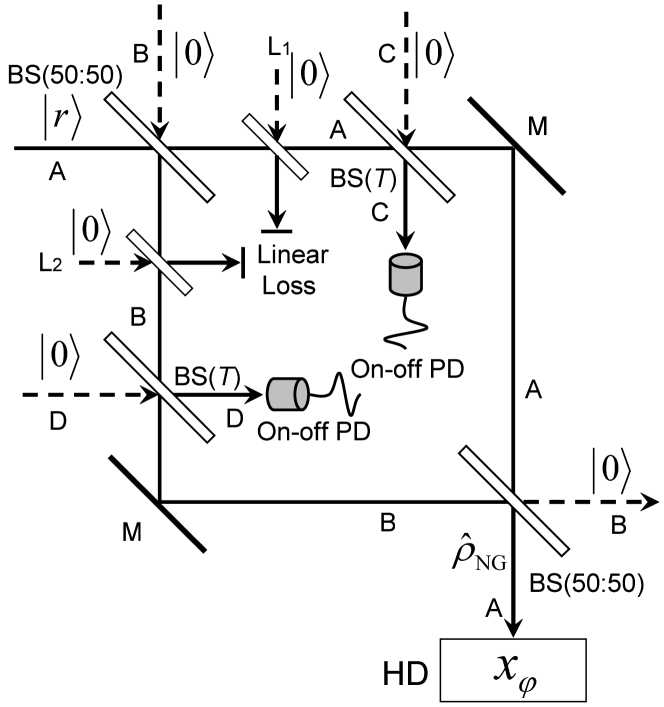
Figure 1: Measurement-induced non-Gaussian operation on the single-mode squeezed vacuum state. BS, PD, M, and HD are beam splitter, photon detector, mirror, and homodyne detection, respectively.

The input squeezed state is divided into two modes A and B with a beam splitter of transmittance $\tau$. Mode C (D) is then tapped from mode A (B) with a beam splitter of high transmittance $T$. The resulting four-mode state is then

$$|\psi_{\rm in}\rangle_{\rm ABCD}=\hat{V}_{\rm BD}(\theta)\hat{V}_{\rm AC}(\theta)\hat{V}_{\rm AB}(\phi)|r\rangle_{\rm A}|0\rangle_{\rm BCD},$$ (4)

where

$$\hat{V}_{kl}(\theta)=\exp\left[\theta(\hat{a}_{k}^{\dagger}\hat{a}_{l}-\hat{a}_{k}\hat{a}_{l}^{\dagger})\right]$$ (5)

is the beam splitting operator, and the parameters $\phi$ and $\theta$ are related with the transmittances $\tau$ and $T$ as

$$\tan\phi=\sqrt{\frac{1-\tau}{\tau}},\ \tan\theta=\sqrt{\frac{1-T}{T}},$$ (6)

respectively. We consider a balanced interferometer $(\tau=0.5)$. Modes C and D are led to the on-off type photon detector. The probability operator valued measure (POVM) of on-off detector is described as

$$\left\{\hat{\Pi}^{(\textrm{on})}_{k}=\hat{1}_{k}-|0\rangle_{k}\langle 0|,\hat{\Pi}^{(\textrm{off})}_{k}=|0\rangle_{k}\langle 0|\right\}.$$ (7)

Simultaneous on events in both modes C and D project the state over mode A and B into the state

$$\hat{\rho}_{\rm out}=\frac{\textrm{Tr}_{\rm CD}\left[|\psi_{\rm in}\rangle_{\rm(ABCD)}\langle\psi_{\rm in}|\otimes\hat{\Pi}^{(\textrm{on})}_{\rm C}\otimes\hat{\Pi}^{(\textrm{on})}_{\rm D}\right]}{P_{\rm det}},$$ (8)

where

$$P_{\rm det} = \textrm{Tr}_{\rm ABCD}\left[|\psi_{\rm in}\rangle_{\rm(ABCD)}\langle\psi_{\rm in}|\otimes\hat{\Pi}^{(\textrm{on})}_{\rm C}\otimes\hat{\Pi}^{(\textrm{on})}_{\rm D}\right]$$ (9)

$$= 1-2\sqrt{\frac{1-\lambda^{2}}{1-\lambda^{2}(\frac{1+T}{2})^{2}}}+\sqrt{\frac{1-\lambda^{2}}{1-\lambda^{2}T^{2}}}$$

is the success probability of this on event selection, and $\lambda\equiv\tanh r$. Finally, remaining modes A and B are recombined with another beam splitter of the transmittance $\tau(=0.5)$, being transformed as

$$\hat{V}_{\rm AB}^{\dagger}(\phi)\hat{\rho}_{\rm out}\hat{V}_{\rm AB}(\phi)=\hat{\rho}_{\rm NG}\otimes|0\rangle_{\rm B}\langle 0|.$$ (10)

The output state of mode B is the vacuum state due to the interference.

The success probability and the quality of the output non-Gaussian state can be controlled by the transmittance of the tapping beam splitter $T$. There is a trade-off between these two. The non-Gaussian property appears more strikingly for higher transmittance but with sacrifice of lower success probability. Hereafter, we set $T=0.9$.

The output non-Gaussian state in mode A is measured by the homodyne detection. The measurement basis is given by the the quadrature eigenstate

$$\hat{x}_{\varphi}|x_{\varphi}\rangle=x_{\varphi}|x_{\varphi}\rangle,$$ (11)

$$|x_{\varphi}\rangle=\frac{1}{\sqrt[4]{\pi}}\exp\left[-\frac{1}{2}x_{\varphi}^{2}+\sqrt{2}e^{i\varphi}x_{\varphi}\hat{a}^{\dagger}-\frac{1}{2}e^{2i\varphi}\hat{a}^{\dagger 2}\right]|0\rangle.$$

(12)

The probability distribution is given by

$$P_{\rm HD}(x_{\varphi};\lambda) = \langle x_{\varphi}|\hat{\rho}_{\rm NG}|x_{\varphi}\rangle$$ (13)

$$= P_{11}(x_{\varphi};\lambda)-P_{10}(x_{\varphi};\lambda)$$

$$\hskip 28.45274pt-P_{01}(x_{\varphi};\lambda)+P_{00}(x_{\varphi};\lambda),$$

where

$$P_{ij}(x_{\varphi};\lambda)$$

$$= \frac{1}{\sqrt{\pi}P_{\rm det}}\sqrt{\frac{1-\lambda^{2}}{(1-\lambda T)^{2}-\lambda^{2}\gamma_{ij}^{2}+4\lambda T\sin^{2}\varphi}}$$

$$\times\exp\left[-\frac{1-\lambda^{2}(T+\gamma_{ij})^{2}}{(1-\lambda T)^{2}-\lambda^{2}\gamma_{ij}^{2}+4\lambda T\sin^{2}\varphi}x_{\varphi}^{2}\right],$$

and $\gamma_{11}=R\equiv 1-T$, $\gamma_{10}=\gamma_{01}=R/2$, and $\gamma_{00}=0$. Thus the probability distribution consists of the four Gaussian terms. Fig. 2 shows the probability distribution of non-Gaussian state ($\lambda=0.4$) along $x_{\varphi=0}\equiv x$ axis (the solid line) and the one of the input squeezed vacuum state (the dotted line).

Figure 2: Probability distribution of the single-mode non-Gaussian state (solid line, $\lambda=0.4$, $T=0.9$) and the squeezed vacuum state (dotted line, $\lambda=0.4$) for the phase parameter $\varphi=0$ with ideal setup.

The probability distribution of the output non-Gaussian state consists of the single main peak with two small side lobes. The probability distribution dominated by the single main peak may still be characterized by the variance

$$V(\lambda)$$ (15)

$$= \int_{-\infty}^{\infty}dx\ x^{2}P_{\rm HD}(x;\lambda)-\left\{\int_{-\infty}^{\infty}dx\ xP_{\rm HD}(x;\lambda)\right\}^{2}$$

$$= V_{11}(\lambda)-V_{10}(\lambda)-V_{01}(\lambda)+V_{00}(\lambda),$$

where

$$V_{ij}(\lambda)=\frac{\sqrt{1-\lambda^{2}}}{2P_{\rm det}}\frac{(1-\lambda T)^{2}-\lambda^{2}\gamma_{ij}^{2}}{\left[1-\lambda^{2}(T+\gamma_{ij})^{2}\right]^{3/2}}$$ (16)

and $\gamma_{ij}$’s have been given above.

Figure 3: Variance of the single-mode non-Gaussian state (solid line, $T=0.9$) and the squeezed vacuum state (dotted line) with ideal setup.

In Fig. 3, the variances of the output non-Gaussian state and of the original input squeezed state are compared. As seen, in the range of $\lambda\lesssim 0.47$, the variance of the output non-Gaussian state is lower than that of original squeezed state, which means that the squeezing degree is effectively enhanced.

Our interferometric non-Gaussian operation scheme is actually found to be equivalent to the Schrödinger cat-like state generation proposed in Ref. Dakna97 (Fig. 4).

Figure 4: Schrödinger cat-like state generation scheme in Ref. Dakna97 . BS, PD, and HD are beam splitter, photon detector, and homodyne detection, respectively.

This can directly be observed by the following equation

$$\hat{V}_{\rm AB}^{\dagger}(\phi)|\psi_{\rm in}\rangle_{\rm ABCD}$$ (17)

$$= \hat{V}_{\rm CD}(\phi)\hat{V}_{\rm AC}(\theta)\hat{V}_{\rm BD}(\theta)\hat{V}_{\rm CD}^{\dagger}(\phi)|r\rangle_{\rm A}|0\rangle_{\rm BCD}$$

$$= \hat{V}_{\rm CD}(\phi)\hat{V}_{\rm AC}(\theta)|r\rangle_{\rm A}|0\rangle_{\rm BCD},$$

by noting that input modes B, C, and D are all the vacuum state.

The Wigner function

$$W(x,p)=\frac{1}{\pi}\int_{-\infty}^{\infty}dye^{-2ipy}\langle x-y|\rho|x+y\rangle$$ (18)

of the non-Gaussian state is obtained by

$$W_{\rm NG}(x,p;\lambda) = W_{11}(x,p;\lambda)-W_{10}(x,p;\lambda)$$ (19)

$$\hskip 5.69054pt-W_{01}(x,p;\lambda)+W_{00}(x,p;\lambda),$$

where

$$W_{ij}(x,p;\lambda) = \frac{1}{\pi P_{\rm det}}\sqrt{\frac{1-\lambda^{2}}{1-\lambda^{2}(T-\gamma_{ij})^{2}}}$$

$$\hskip 8.53581pt\times\exp\left[-\frac{1-\lambda^{2}(T+\gamma_{ij})^{2}}{(1-\lambda T)^{2}-\lambda^{2}\gamma_{ij}^{2}}x^{2}\right]$$

$$\hskip 17.07164pt\times\exp\left[-\frac{(1-\lambda T)^{2}-\lambda^{2}\gamma_{ij}^{2}}{1-\lambda^{2}(T-\gamma_{ij})^{2}}p^{2}\right].$$

This is illustrated for two $\lambda$’s in Figs. 5 ($\lambda=0.4$) and 6 ($\lambda=0.8$).

Figure 5: Wigner function of the single-mode non-Gaussian state ($\lambda=0.4$, $T=0.9$) with ideal setup.

Figure 6: Wigner function of the single-mode non-Gaussian state ($\lambda=0.8$, $T=0.9$) with ideal setup.

For smaller $\lambda$, the Wigner function is closer to that of the squeezed vacuum state. For larger $\lambda$, on the other hand, the property of cat-like state becomes more remarkable. These figures will be compared later with the case including imperfections.

Interestingly, the average photon number

$$\bar{N}(\lambda) = \textrm{Tr}\left[\hat{\rho}_{\rm NG}\otimes\hat{N}\right]$$ (21)

$$= N_{11}(\lambda)-N_{10}(\lambda)-N_{01}(\lambda)+N_{00}(\lambda)$$

increases after conditional non-Gaussian operation (Fig. 7), where $\hat{N}=\hat{a}^{\dagger}\hat{a}$ is the photon number operator, and

$$N_{ij}(\lambda)=\frac{1}{P_{\rm det}}\sqrt{\frac{1-\lambda^{2}}{1-\lambda^{2}(T+\gamma_{ij})^{2}}}\frac{\lambda^{2}T(T+\gamma_{ij})}{1-\lambda^{2}(T+\gamma_{ij})^{2}}.$$ (22)

Figure 7: Average photon number of the single-mode non-Gaussian state (solid line, $T=0.9$) and the squeezed vacuum state (dotted line) with ideal setup.

III Non-Gaussian operation on two-mode squeezed state

Now we turn to the two-mode case (Fig. 8) in the ideal situation, where the other squeezed vacuum state with the reduced uncertainty of the $p$ $(\equiv x_{\varphi+\frac{\pi}{2}})$-quadrature is input into mode B instead of the vacuum state.

Figure 8: Measurement-induced non-Gaussian operation on the two-mode squeezed vacuum state. BS, PD, M, and HD are beam splitter, photon detector, mirror, and homodyne detection, respectively.

The two-mode squeezed vacuum state

$$|r^{(2)}\rangle_{\rm AB} = \hat{V}_{\rm AB}\left(\frac{\pi}{4}\right)|r\rangle_{\rm A}|-r\rangle_{\rm B}$$ (23)

$$\equiv \hat{S}^{(2)}_{\rm AB}(-r)|0\rangle_{\rm AB},$$

is generated after the first 50:50 beam splitter, where

$$\hat{S}^{(2)}_{kl}(r)=\exp\left[-r(\hat{a}_{k}^{\dagger}\hat{a}_{l}^{\dagger}-\hat{a}_{k}\hat{a}_{l})\right]$$ (24)

is the two-mode squeezing operator. The operations after this is similar to the single-mode case. The state conditioned by the simultaneous $on$ results for modes C and D is

$$\hat{\rho}_{\rm NG}^{(2)}=\frac{\textrm{Tr}_{\rm CD}\left[|\psi_{\rm in}^{(2)}\rangle_{\rm(ABCD)}\langle\psi_{\rm in}^{(2)}|\otimes\hat{\Pi}^{(\textrm{on})}_{\rm C}\otimes\hat{\Pi}^{(\textrm{on})}_{\rm D}\right]}{P_{\rm det}^{(2)}},$$ (25)

where

$$|\psi_{\rm in}^{(2)}\rangle_{\rm ABCD}=\hat{V}_{\rm AC}(\theta)\hat{V}_{\rm BD}(\theta)|r^{(2)}\rangle_{\rm AB}|0\rangle_{\rm CD},$$ (26)

with the high transemittance $T=\cos^{2}\theta$, and

$$P_{\rm det}^{(2)} = \textrm{Tr}_{\rm ABCD}\left[|\psi_{\rm in}^{(2)}\rangle_{\rm(ABCD)}\langle\psi_{\rm in}^{(2)}|\otimes\hat{\Pi}^{(\textrm{on})}_{\rm C}\otimes\hat{\Pi}^{(\textrm{on})}_{\rm D}\right]$$ (27)

$$= \frac{\lambda^{2}(1-T)^{2}(1+\lambda^{2}T)}{(1-\lambda^{2}T)(1-\lambda^{2}T^{2})}$$

is the success probability of the $on$ event selection.

The two modes of the conditional non-Gaussian entangled state are combined via the second 50:50 beam splitter, and are then measured by the two homodyne detectors, each of which measures the two orthogonal quadratures simultaneously. This chain of operations corresponds to the CV Bell measurement represented by

$$|\Pi(x,p)\rangle_{kl}=\frac{1}{\sqrt{2\pi}}\int_{-\infty}^{\infty}dye^{ipy}|x+y\rangle_{k}|y\rangle_{l}.$$ (28)

Therefore, the probability distribution of homodyne detection in phase space is

$$P_{\rm HD}^{(2)}(x,p;\lambda) = \langle\Pi(x,p)|\hat{\rho}_{\rm NG}^{(2)}|\Pi(x,p)\rangle$$ (29)

$$= P_{11}^{(2)}(x,p;\lambda)-P_{10}^{(2)}(x,p;\lambda)$$

$$\hskip 5.69054pt-P_{01}^{(2)}(x,p;\lambda)+P_{00}^{(2)}(x,p;\lambda),$$

where

$$P_{ij}^{(2)}(x,p;\lambda)$$

$$= \frac{1}{2\pi P_{\rm det}^{(2)}}\frac{1-\lambda^{2}}{(1-\lambda T)^{2}-\lambda^{2}\gamma_{i}^{(2)}\gamma_{j}^{(2)}}$$

$$\hskip 5.69054pt\times\exp\left[-\frac{1-\lambda^{2}(T+\gamma_{1}^{(2)})(T+\gamma_{2}^{(2)})}{2\{(1-\lambda T)^{2}-\lambda^{2}\gamma_{i}^{(2)}\gamma_{j}^{(2)}\}}(x^{2}+p^{2})\right],$$

and $\gamma_{1}^{(2)}=R$, $\gamma_{0}^{(2)}=0$. We can see that Eq. (29) is also the combination of four Gaussian terms, which is totally non-Gaussian distribution. Fig. 9 shows the probability distribution $P_{\rm HD}^{(2)}(x,p;\lambda)$ along $x$ axis for $\lambda=0.4$, after integrating out the variable $p$.

Figure 9: Probability distribution of the two-mode non-Gaussian state (solid line, $\lambda=0.4$, $T=0.9$) and the squeezed vacuum state (dotted line, $\lambda=0.4$) for the phase parameter $\varphi=0$ on the mode A with ideal setup. Probability distribution for $\varphi=\pi/2$ on the mode B gives the same result.

In this two mode case, the two small side lobes cannot be seen, and the distribution is close to Gaussian. This distribution may be characterized by its variance,

$$V^{(2)}(\lambda)$$ (31)

$$= \int_{-\infty}^{\infty}dp\int_{-\infty}^{\infty}dx\ x^{2}P_{\rm HD}^{(2)}(x,p;\lambda)$$

$$\hskip 56.9055pt-\left\{\int_{-\infty}^{\infty}dp\int_{-\infty}^{\infty}dx\ xP_{\rm HD}^{(2)}(x,p;\lambda)\right\}^{2}$$

$$= V_{11}^{(2)}(\lambda)-V_{10}^{(2)}(\lambda)-V_{01}^{(2)}(\lambda)+V_{00}^{(2)}(\lambda),$$

where

$$V_{ij}^{(2)}(\lambda)=\frac{1}{P_{\rm det}^{(2)}}\frac{(1-\lambda^{2})\{(1-\lambda T)^{2}-\lambda^{2}\gamma_{i}^{(2)}\gamma_{j}^{(2)}\}}{[1-\lambda^{2}(T+\gamma_{i}^{(2)})(T+\gamma_{j}^{(2)})]^{2}}.$$ (32)

This is shown in Fig. 10 by the solid line. The dotted line corresponds to the case of the two-mode squeezed vacuum state.

Figure 10: Variance of the two-mode non-Gaussian state (solid line, $T=0.9$) and the squeezed vacuum state (dotted line) with ideal setup.

In $\lambda\lesssim 0.67$, the variance of two-mode non-Gaussian state is lower than that of two-mode squeezed vacuum state. Thus the squeezing degree is effectively enhanced in the two-mode case as well. The measurement on CV Bell basis (28) is one of the correlation between two modes, therefore we can consider the variance (31) as a measure of quantum correlation of bipartite entangled pair.

IV Application to dense coding scheme

The entanglement measures for CV systems have been clarified for Gaussian states so far. But the measures for mixed non-Gaussian states are not clear yet. In this regards, it might be sensible to adopt some operational measures connected directly to CV protocols. In this section, we evaluate the property of the conditional non-Gaussian state in terms of the mutual information for the dense coding scheme proposed in Ban99 ; Braunstein00 . The result here is added to the ones based on the other kinds of operational measures, such as the improvement of the teleportation fidelity Olivares03 and the nonlocality due to the violation of Bell type inequality Nha04 ; Garcia-Patron04PRL ; Garcia-Patron04 ; Olivares04 .

The variance reduction of the non-Gaussian states shown in the previous section implies the improvement of the signal-to-noise ratio, and hence the increase of the transmissible information. This can be measured by mutual information, which is calculated by evaluating the channel matrix between the input and output signals. This measure is known to be a stringent figure of merit for the system in the sense that the gain usually vanishes even with relatively small imperfections. Therefore it would be a nice criterion to see whether the information gain is observed or not by the non-Gaussian operation compared with the original two-mode squeezed vacuum state.

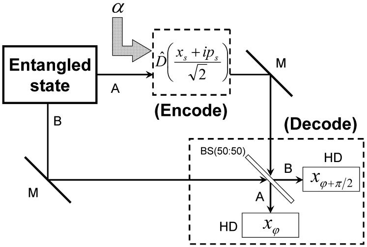
Figure 11: The setup of dense coding scheme with power of signal modulation $\alpha$. BS, M, and HD means beam splitter, mirror, and homodyne detection, respectively.

In Fig. 11, the setup of dense coding scheme is depicted. Alice encodes classical message $(x_{s},p_{s})$ on one of the beam of the two-mode non-Gaussian entangled state by the displacement operation,

$$\hat{U}_{\rm A}(x_{s},p_{s}) = e^{-\frac{i}{2}x_{s}p_{s}}\hat{D}\left(\frac{x_{s}+ip_{s}}{\sqrt{2}}\right)$$ (33)

$$= e^{-ip_{s}\hat{x}_{\rm A}}e^{ix_{s}\hat{p}_{\rm A}},$$

where $\hat{D}(\alpha)\equiv\exp(\alpha\hat{a}^{\dagger}-\alpha^{\ast}\hat{a})$. Now, we consider a simple model in which signals $x_{s}$ and $p_{s}$ are restricted to $\pm\sqrt{2}\alpha$ with equal prior probabilities, (quadrature phase shift keying) and thus a set of 2-bit information $\{a_{00}=(x_{s}\equiv\sqrt{2}\alpha,p_{s}\equiv\sqrt{2}\alpha),\,a_{01}=(\sqrt{2}\alpha,-\sqrt{2}\alpha),\,a_{10}=(-\sqrt{2}\alpha,\sqrt{2}\alpha),\,a_{11}=(-\sqrt{2}\alpha,-\sqrt{2}\alpha)\}$ is encoded. (The continuous encoding onto the non-Gaussian entangled state makes the calculation difficult, so we have here simplified to the 4 valued discrete encoding. )

Bob attempts to decode classical message from Alice $(x_{s},p_{s})$ by the CV Bell measurement described in Eq. (28). The distribution of the detection probability is given by

$$\langle\Pi(x,p)|\hat{U}_{\rm A}(x_{s},p_{s})\hat{\rho}_{\rm NG}^{(2)}\hat{U}_{\rm A}^{\dagger}(x_{s},p_{s})|\Pi(x,p)\rangle$$ (34)

$$\hskip 85.35826pt=P_{\rm HD}^{(2)}(x-x_{s},p-p_{s};\lambda)$$

$$\hskip 85.35826pt\equiv P(x,p|x_{s},p_{s}),$$

where we use the relation

$$\hat{U}_{\rm A}^{\dagger}(x_{s},p_{s})|\Pi(x,p)\rangle=e^{-ip_{s}(x-x_{s})}|\Pi(x-x_{s},p-p_{s})\rangle.$$ (35)

Then Bob identifies the 2-bit classical messages according to the decision rule $\{b_{00}=(x\geq 0,p\geq 0),\,b_{01}=(x\geq 0,p<0),\,b_{10}=(x<0,p\geq 0),\,b_{11}=(x<0,p<0)\}$.

Now the 4-by-4 channel matrix is given by $\{P(a_{mn}|b_{kl})\}$ where the elements for ($m=k,n=l$) contribute to the success probability and otherwise, the error probability. For example,

$$P(b_{00}|a_{00})$$ (36)

$$=\int_{0}^{\infty}dx\int_{0}^{\infty}dpP(x,p|\sqrt{2}\alpha,\sqrt{2}\alpha)$$

$$=\sum_{i,j=0}^{1}\frac{1}{4P_{\rm det}^{(2)}}\frac{1-\lambda^{2}}{1-\lambda^{2}(T+\gamma^{(2)}_{i})(T+\gamma^{(2)}_{j})}$$

$$\hskip 85.35826pt\times\left(1+\textrm{erf}\left[\Omega_{ij}(\lambda)\alpha\right]\right)^{2}$$

where

$$\Omega_{ij}(\lambda)=\sqrt{\frac{1-\lambda^{2}(T+\gamma^{(2)}_{i})(T+\gamma^{(2)}_{j})}{(1-\lambda T)^{2}-\lambda^{2}\gamma^{(2)}_{i}\gamma^{(2)}_{j}}}$$ (37)

and

$$\textrm{erf}\ \!(x)=\frac{2}{\sqrt{\pi}}\int_{0}^{x}dte^{-t^{2}}$$ (38)

is the error function. Other components can be obtained similarly,

$$P(b_{mn}|a_{kl})$$ (39)

$$=\sum_{i,j=0}^{1}\frac{1}{4P_{\rm det}^{(2)}}\frac{1-\lambda^{2}}{1-\lambda^{2}(T+\gamma^{(2)}_{i})(T+\gamma^{(2)}_{j})}$$

$$\hskip 28.45274pt\times\left(1+(-1)^{m-k}\textrm{erf}\left[\Omega_{ij}(\lambda)\alpha\right]\right)$$

$$\hskip 56.9055pt\times\left(1+(-1)^{n-l}\textrm{erf}\left[\Omega_{ij}(\lambda)\alpha\right]\right).$$

The mutual information is calculated by the above channel matrix as

$$I(\textrm{A};\textrm{B})$$ (40)

$$=\sum_{k,l,m,n}P(a_{kl})P(b_{mn}|a_{kl})$$

$$\hskip 28.45274pt\times\log_{2}\left[\frac{P(b_{mn}|a_{kl})}{\displaystyle\sum_{k,l}P(a_{kl})P(b_{mn}|a_{kl})}\right]$$

$$\rightarrow 2\ [\textrm{bit}]\quad\textrm{as}\ \lambda\rightarrow 1,$$

where $P(a_{kl})=1/4$ is the prior probability.

From the viewpoint of communication efficiency, we should optimize the mutual information under the power constraint condition that the total energy of initial squeezing power and encoding displacement power is constant. We are, however, interested in how to quantify the improvement brought by the entanglement enhancement due to the non-Gaussian operation for a given input. What should be fixed is then the degree of entanglement of the input state, equivalently the squeezing degree $\lambda$ for the input. We intend to compare the mutual informations between the cases with and without the non-Gaussian operation.

In Figs. 12 and 13, the mutual information of $\alpha=1.5$ and $\alpha=0.7$ are indicated respectively, where the original squeezed vacuum state cases are also indicated by the dotted line.

Figure 12: Mutual information via the dense coding channel ($\alpha=1.5$) of the non-Gaussian state (solid line, $T=0.9$) and the squeezed vacuum state (dotted line) with ideal setup.

Figure 13: Mutual information via the dense coding channel ($\alpha=0.7$) of the non-Gaussian state (solid line, $T=0.9$) and the squeezed vacuum state (dotted line) with ideal setup.

We can see that, in the range of $\lambda\lesssim 0.38$ and $\lambda\lesssim 0.65$, in Fig. 12 and 13, respectively, the mutual information of two-mode non-Gaussian state is larger than the original two-mode squeezed vacuum state case. This can naturally be regarded as the gain assisted by the enhanced entanglement of the non-Gaussian entangled state. Via the probabilistic photon subtraction operation, similar to the single-mode case, the average photon number of output two-mode non-Gaussian state increases compared with input squeezed vacuum state, which brings effective enhancement of entanglement.

V POVM of practical photon detector model

From this section, we consider possible imperfections, including the linear loss in optical paths, finite quantum efficiency and nonzero dark counts of the on-off detector. The imperfect photon detector may be modeled by the following POVM element Barnett98 ,

$$\hat{\Pi}(m;\eta)=\sum_{n=m}^{\infty}\binom{n}{m}\eta^{m}(1-\eta)^{n-m}|n\rangle\langle n|,$$ (41)

where $n$ photons are converted to $m\leq n$ with the imperfect quantum efficiency $\eta$, and

$$\binom{n}{m}=\frac{n!}{(n-m)!m!}$$ (42)

is the binomial coefficient. This element is considered as the sequence of two devices; beam splitter of transmittance $\eta$ (linear loss) and perfect $n$ photon counting detector, where $n-m$ photons are removed as the linear loss. As a whole, $m$ photons are detected.

Further, assume that the net count of photon detector is $N(\geq m)$, where $N-m$ photons are due to dark count, following Poisson distribution. With average dark count $\nu$, the POVM of detector counting $N$ photons is

$$\hat{\Pi}(N,\eta,\nu)$$

$$=\sum_{m=0}^{N}e^{-\nu}\frac{\nu^{N-m}}{(N-m)!}\sum_{n=m}^{\infty}\binom{n}{m}\eta^{m}(1-\eta)^{n-m}|n\rangle\langle n|,$$

which satisfies completeness relation,

$$\sum_{N=0}^{\infty}\hat{\Pi}(N,\eta,\nu)=\hat{1}.$$ (44)

With Eqs. (LABEL:POVM-N) and (44), we obtain a set of POVM’s of practical on-off type photon detector,

$$\left\{\hat{\Pi}^{(\textrm{off})}(\eta,\nu),\hat{\Pi}^{(\textrm{on})}(\eta,\nu)\right\},$$ (45)

where

$$\hat{\Pi}^{(\textrm{off})}(\eta,\nu) = \hat{\Pi}(0,\eta,\nu)$$ (46)

$$= e^{-\nu}\sum_{n=0}^{\infty}(1-\eta)^{n}|n\rangle\langle n|,$$

$$\hat{\Pi}^{(\textrm{on})}(\eta,\nu) = \sum_{N=1}^{\infty}\hat{\Pi}(N,\eta,\nu)$$ (47)

$$= \hat{1}-\hat{\Pi}^{(\textrm{off})}(\eta,\nu).$$

VI Analysis with practical parameters in single-mode scheme

Let us first go with the single-mode non-Gaussian operation (Fig. 1). The quantum efficiency of the homodyne detector may be considered as approximately the unity, which is the case of the time limited signals prepared by chopping the continuous wave field generated from the cavity enhanced optical parametric process. We assume that the linear loss occurs between the first and second beam splitters, which may be attributed to the loss on beam splitters, mirrors, nonlinear crystals. Such a decohered squeezed vacuum state is transformed into the non-Gaussian state by the imperfect on-off type photon detectors modeled above.

The linear loss in optical paths can be described with a beam splitter of transmittance $T_{L}$,

$$|\psi_{\rm in}^{\prime}\rangle_{\rm ABCDL_{1}L_{2}}$$ (48)

$$=\hat{V}_{\rm BD}(\theta)\hat{V}_{\rm AC}(\theta)\hat{V}_{\rm BL_{2}}(\xi)\hat{V}_{\rm AL_{1}}(\xi)$$

$$\hskip 56.9055pt\times\hat{V}_{\rm AB}\left(\frac{\pi}{4}\right)|r\rangle_{\rm A}|0\rangle_{\rm BCDL_{1}L_{2}}$$

where $L_{1}$ and $L_{2}$ are assigned for loss channels and

$$\tan\xi=\sqrt{\frac{1-T_{L}}{T_{L}}}.$$ (49)

Modes of $L_{1}$ and $L_{2}$ are traced out, and mode C (D) is tapped from mode A (B) by a beam splitter of high transmittance $T$ respectively. Therefore input state is

$$\hat{\varrho}_{\rm in}=\textrm{Tr}_{\rm L_{1}L_{2}}\left[|\psi^{\prime}_{\rm in}\rangle_{\rm(ABCDL_{1}L_{2})}\langle\psi^{\prime}_{\rm in}|\right].$$ (50)

Then, simultaneous on events on modes C and D are selected conditionally,

$$\hat{\varrho}_{\rm out}=\frac{\textrm{Tr}_{\rm CD}\left[\hat{\varrho}_{\rm in}\otimes\hat{\Pi}^{(\textrm{on})}_{\rm C}(\eta,\nu)\otimes\hat{\Pi}^{(\textrm{on})}_{\rm D}(\eta,\nu)\right]}{{\cal P}_{\rm det}},$$ (51)

where

$${\cal P}_{\rm det} = \textrm{Tr}_{\rm ABCD}\left[\hat{\varrho}_{\rm in}\otimes\hat{\Pi}^{(\textrm{on})}_{\rm C}(\eta,\nu)\otimes\hat{\Pi}^{(\textrm{on})}_{\rm D}(\eta,\nu)\right]$$

$$= 1-2e^{-\nu}\sqrt{\frac{1-\lambda^{2}}{1-\lambda^{2}(T_{L}T+R_{L}+\frac{2-\eta}{2}T_{L}R)^{2}}}$$

$$+e^{-2\nu}\sqrt{\frac{1-\lambda^{2}}{1-\lambda^{2}\{T_{L}T+R_{L}+(1-\eta)T_{L}R\}^{2}}}$$

is the success probability of event selection ($R_{L}\equiv 1-T_{L}$). Then we recombine modes A and B with another balanced beam splitter and mode A is measured with homodyne detection (mode B is vacuum state),

$${\cal P}_{\rm HD}(x_{\varphi};\lambda) = \langle x_{\varphi}|\hat{\varrho}_{\rm NG}|x_{\varphi}\rangle$$

$$= {\cal P}_{11}(x_{\varphi};\lambda)-e^{-\nu}{\cal P}_{10}(x_{\varphi};\lambda)$$

$$\hskip 5.69054pt-e^{-\nu}{\cal P}_{01}(x_{\varphi};\lambda)+e^{-2\nu}{\cal P}_{00}(x_{\varphi};\lambda),$$

where

$$\hat{\varrho}_{\rm NG} = \hat{V}_{\rm AB}^{\dagger}\left(\frac{\pi}{4}\right)\hat{\varrho}_{\rm out}\hat{V}_{\rm AB}\left(\frac{\pi}{4}\right),$$ (54)

$${\cal P}_{ij}(x_{\varphi};\lambda) = \frac{1}{\sqrt{\pi}{\cal P}_{\rm det}}\sqrt{\frac{1-\lambda^{2}}{(1-\lambda T_{L}T)^{2}-\lambda^{2}(R_{L}+\gamma^{\prime}_{ij})^{2}+4\lambda T_{L}T\sin^{2}\varphi}}$$ (55)

$$\hskip 85.35826pt\times\exp\left[-\frac{1-\lambda^{2}(T_{L}T+R_{L}+\gamma^{\prime}_{ij})^{2}}{(1-\lambda T_{L}T)^{2}-\lambda^{2}(R_{L}+\gamma^{\prime}_{ij})^{2}+4\lambda T_{L}T\sin^{2}\varphi}x_{\varphi}^{2}\right],$$

and $\gamma^{\prime}_{11}=T_{L}R$, $\gamma^{\prime}_{10}=\gamma^{\prime}_{01}=(2-\eta)T_{L}R/2$, and $\gamma^{\prime}_{00}=(1-\eta)T_{L}R$. With above results, we can obtain the variance of non-Gaussian state along $x$ axis ($\varphi=0$),

$${\cal V}(\lambda)$$

$$= \int_{-\infty}^{\infty}dx\ x^{2}{\cal P}_{\rm HD}(x;\lambda)-\left\{\int_{-\infty}^{\infty}dx\ x{\cal P}_{\rm HD}(x;\lambda)\right\}^{2}$$

$$= {\cal V}_{11}(\lambda)-e^{-\nu}{\cal V}_{10}(\lambda)-e^{-\nu}{\cal V}_{01}(\lambda)+e^{-2\nu}{\cal V}_{00}(\lambda),$$

where

$${\cal V}_{ij}(\lambda) = \frac{1}{2{\cal P}_{\rm det}}\sqrt{\frac{1-\lambda^{2}}{1-\lambda^{2}(T_{L}T+R_{L}+\gamma^{\prime}_{ij})^{2}}}$$ (57)

$$\hskip 14.22636pt\times\frac{(1-\lambda T_{L}T)^{2}-\lambda^{2}(R_{L}+\gamma^{\prime}_{ij})^{2}}{1-\lambda^{2}(T_{L}T+R_{L}+\gamma^{\prime}_{ij})^{2}}.$$

We assume the total linear loss 25% ($T_{L}=0.75$), and the on-off type detector of quantum efficiency $\eta=0.6$ and the dark count rate 10000 [counts/sec]. At present, lower dark count rate $\sim 100$ [counts/sec] is achievable in laboratory, however, we consider the rather large value to see the effect more clearly. When the gating time of photon detector is $10^{-7}$ [sec], the net dark count in a single event is $\nu=10^{-3}$, which is large enough to affect the output state.

Figure 14 shows the probability distribution of non-Gaussian state ($\lambda=0.4$) along $x$ axis (solid line) and the one of the input squeezed vacuum state (dotted line), where the two side lobes seen in Fig. 2 disappear due to imperfections. In Fig. 15, the variances of the output non-Gaussian state and of the original input squeezed state are compared. The reduction of the variance due to the non-Gaussian operation is seen for $\lambda\lesssim 0.4$. At this cross point, the variance shows 2.5 dB (in terms of $-10\log_{10}\left[{\cal V}(\lambda)/{\cal V}(0)\right][\textrm{dB}]$) below the shot noise level. The range of the variance suppression becomes narrower than the ideal case where $\lambda\lesssim 0.47$ (Fig. 3). This is mainly due to the dark counts. The linear loss spoils the degree of squeezing, as the increase of the overall variance level. The imperfect quantum efficiency reduces success probability ${\cal P}_{\rm det}$.

Figure 14: Probability distribution of the single-mode non-Gaussian state (solid line, $\lambda=0.4$, $T=0.9$) and the squeezed vacuum state (dotted line, $\lambda=0.4$) for the phase parameter $\varphi=0$ with practical setup ($T_{L}=0.75$, $\eta=0.6$, $\nu=10^{-3}$).

Figure 15: Variance of the single-mode non-Gaussian state (solid line, $T=0.9$) and the squeezed vacuum state (dotted line) with practical setup ($T_{L}=0.75$, $\eta=0.6$, $\nu=10^{-3}$).

The Wigner function of the non-Gaussian state in the imperfect setup is calculated as

$${\cal W}_{\rm NG}(x,p;\lambda)$$ (58)

$$= {\cal W}_{11}(x,p;\lambda)-e^{-\nu}{\cal W}_{10}(x,p;\lambda)$$

$$\hskip 28.45274pt-e^{-\nu}{\cal W}_{01}(x,p;\lambda)+e^{-2\nu}{\cal W}_{00}(x,p;\lambda),$$

where

$${\cal W}_{ij}(x,p;\lambda)$$ (59)

$$= \frac{1}{\pi{\cal P}_{\rm det}}\sqrt{\frac{1-\lambda^{2}}{1-\lambda^{2}(T_{L}T-R_{L}-\gamma^{\prime}_{ij})^{2}}}$$

$$\hskip 2.84526pt\times\exp\left[-\frac{1-\lambda^{2}(T_{L}T+R_{L}+\gamma^{\prime}_{ij})^{2}}{(1-\lambda T_{L}T)^{2}-\lambda^{2}(R_{L}+\gamma^{\prime}_{ij})^{2}}x^{2}\right]$$

$$\hskip 8.53581pt\times\exp\left[-\frac{(1-\lambda T_{L}T)^{2}-\lambda^{2}(R_{L}+\gamma^{\prime}_{ij})^{2}}{1-\lambda^{2}(T_{L}T-R_{L}-\gamma^{\prime}_{ij})^{2}}p^{2}\right].$$

The Wigner functions for $\lambda=0.4$ and $\lambda=0.8$ are illustrated in Figs. 16 and 17, respectively. The former is still similar to the squeezed state, while the latter is close to decohered plus-cat state, compared with Figs. 5 and 6.

Figure 16: Wigner function of the single-mode non-Gaussian state ($\lambda=0.4$, $T=0.9$) with practical setup ($T_{L}=0.75$, $\eta=0.6$, $\nu=10^{-3}$).

Figure 17: Wigner function of the single-mode non-Gaussian state ($\lambda=0.8$, $T=0.9$) with practical setup ($T_{L}=0.75$, $\eta=0.6$, $\nu=10^{-3}$).

VII Analysis with practical parameters in two-mode scheme

We turn to the analysis of two-mode scheme with practical parameters (Fig. 8). Similar to the single-mode case, we assume that the linear loss occurs between the first and second beam splitters, and model the effect by inserting a beam splitter of transmittance $T_{L}$ into each arm. The resulting state is then

$$\hat{\varrho}_{\rm in}^{(2)}=\textrm{Tr}_{\rm L_{1}L_{2}}\left[|\psi^{\prime(2)}_{\rm in}\rangle_{\rm(ABCDL_{1}L_{2})}\langle\psi^{\prime(2)}_{\rm in}|\right],$$ (60)

where

$$|\psi^{\prime(2)}_{\rm in}\rangle_{\rm ABCDL_{1}L_{2}}$$ (61)

$$= \hat{V}_{\rm BD}(\theta)\hat{V}_{\rm AC}(\theta)\hat{V}_{\rm BL_{2}}(\xi)\hat{V}_{\rm AL_{1}}(\xi)\hat{V}_{\rm AB}\left(\frac{\pi}{4}\right)$$

$$\hskip 71.13188pt\times|r\rangle_{\rm A}|-r\rangle_{\rm B}|0\rangle_{\rm CDL_{1}L_{2}}.$$

The conditional state selected by simultaneous on events on modes C and D is then,

$$\hat{\varrho}_{\rm NG}^{(2)}=\frac{\textrm{Tr}_{\rm CD}\left[\hat{\varrho}_{\rm in}^{(2)}\otimes\hat{\Pi}_{\rm C}^{(\textrm{on})}\otimes\hat{\Pi}_{\rm D}^{(\textrm{on})}\right]}{{\cal P}_{\rm det}^{(2)}},$$ (62)

where

$${\cal P}_{\rm det}^{(2)} = 1-2e^{-\nu}\frac{1-\lambda^{2}}{1-\lambda^{2}\{1-\eta T_{L}(1-T)\}}$$ (63)

$$\hskip 14.22636pt+e^{-2\nu}\frac{1-\lambda^{2}}{1-\lambda^{2}\{1-\eta T_{L}(1-T)\}^{2}}$$

is the success probability of this event selection. The probability distribution of the Bell measurement is

$${\cal P}_{\rm HD}^{(2)}(x,p;\lambda)$$ (64)

$$= \langle\Pi(x,p)|\hat{\varrho}_{\rm NG}^{(2)}|\Pi(x,p)\rangle$$

$$= {\cal P}_{11}^{(2)}(x,p;\lambda)-e^{-\nu}{\cal P}_{10}^{(2)}(x,p;\lambda)$$

$$\hskip 14.22636pt-e^{-\nu}{\cal P}_{01}^{(2)}(x,p;\lambda)+e^{-2\nu}{\cal P}_{00}^{(2)}(x,p;\lambda),$$

where

$${\cal P}_{ij}^{(2)}(x,p;\lambda) = \frac{1}{2\pi{\cal P}_{\rm det}^{(2)}}\frac{1-\lambda^{2}}{(1-\lambda T_{L}T)^{2}-\lambda^{2}(R_{L}+\gamma^{\prime(2)}_{i})(R_{L}+\gamma^{\prime(2)}_{j})}$$ (65)

$$\hskip 56.9055pt\times\exp\left[-\frac{1-\lambda^{2}(T_{L}T+R_{L}+\gamma^{\prime(2)}_{i})(T_{L}T+R_{L}+\gamma^{\prime(2)}_{j})}{2\{(1-\lambda T_{L}T)^{2}-\lambda^{2}(R_{L}+\gamma^{\prime(2)}_{i})(R_{L}+\gamma^{\prime(2)}_{j})\}}(x^{2}+p^{2})\right],$$

and $\gamma^{\prime(2)}_{1}=T_{L}R$, $\gamma^{\prime(2)}_{0}=(1-\eta)T_{L}R$. With Eqs. (64) and (65), we can calculate the variance of the output state at each port,

$${\cal V}^{(2)}(\lambda)={\cal V}_{11}^{(2)}(\lambda)-e^{-\nu}{\cal V}_{10}^{(2)}(\lambda)-e^{-\nu}{\cal V}_{01}^{(2)}(\lambda)+e^{-2\nu}{\cal V}_{00}^{(2)}(\lambda),$$ (66)

where

$${\cal V}_{ij}^{(2)}(\lambda)=\frac{1}{{\cal P}_{\rm det}^{(2)}}\frac{(1-\lambda^{2})\{(1-\lambda T_{L}T)^{2}-\lambda^{2}(R_{L}+\gamma^{\prime(2)}_{i})(R_{L}+\gamma^{\prime(2)}_{j})\}}{\{1-\lambda^{2}(T_{L}T+R_{L}+\gamma^{\prime(2)}_{i})(T_{L}T+R_{L}+\gamma^{\prime(2)}_{j})\}^{2}}.$$ (67)

Fig. 18 shows the probability distribution of the output non-Gaussian state ${\cal P}_{\rm HD}^{(2)}(x,p;\lambda)$ along $x$ axis for $\lambda=0.4$ (solid line), after the integrating out the variable $p$. We can see that the peak is sharper than the input squeezed vacuum state of $\lambda=0.4$ (dotted line). The variance of the output non-Gaussian state ${\cal V}(\lambda)$ is shown in Fig. 19. Its variance becomes lower in the range of $\lambda\lesssim 0.63$ than that of the input squeezed vacuum state (dotted line), which corresponds to the range up to 3.8 [dB] in the relative decibel scale.

Figure 18: Probability distribution of the two-mode non-Gaussian state (solid line, $\lambda=0.4$, $T=0.9$) and the squeezed vacuum state (dotted line, $\lambda=0.4$) for the phase parameter $\varphi=0$ on the mode A with practical setup ($T_{L}=0.75$, $\eta=0.6$, $\nu=10^{-3}$). Probability distribution for $\varphi=\pi/2$ on the mode B gives the same result.

Figure 19: Variance of the two-mode non-Gaussian state (solid line, $T=0.9$) and the squeezed vacuum state (dotted line) with practical setup ($T_{L}=0.75$, $\eta=0.6$, $\nu=10^{-3}$).

Now, let us consider the dense coding scheme with the two-mode non-Gaussian state (60) in accordance with Sec. IV. We assume that the decoherence of the encoded signals in the way from Alice to Bob is negligible. Actually we are interested in quantifying the effect of non-Gaussian state in terms of the mutual information rather than in applying the scheme to practical communications. The procedure goes in a similar way to the ideal case (Fig. 11).

$$\langle\Pi(x,p)|\hat{U}_{\rm A}(x_{s},p_{s})\hat{\varrho}_{\rm NG}^{(2)}\hat{U}_{\rm A}^{\dagger}(x_{s},p_{s})|\Pi(x,p)\rangle$$ (68)

$$\hskip 85.35826pt={\cal P}_{\rm HD}^{(2)}(x-x_{s},p-p_{s};\lambda).$$

With Eq. (68), we can obtain the channel matrix similar to Eq. (36) and the mutual information can be obtained,

$${\cal I}(\textrm{A};\textrm{B})$$ (69)

$$=\sum_{k,l,m,n}P(a_{kl}){\cal P}(b_{mn}|a_{kl})$$

$$\hskip 28.45274pt\times\log_{2}\left[\frac{{\cal P}(b_{mn}|a_{kl})}{\displaystyle\sum_{k,l}P(a_{kl}){\cal P}(b_{mn}|a_{kl})}\right],$$

where

$${\cal P}(b_{mn}|a_{kl}) = \sum_{i,j=0}^{1}\frac{1}{4{\cal P}_{\rm det}^{(2)}}\frac{1-\lambda^{2}}{1-\lambda^{2}(T_{L}T+R_{L}+\gamma^{\prime(2)}_{i})(T_{L}T+R_{L}+\gamma^{\prime(2)}_{j})}$$ (70)

$$\hskip 85.35826pt\times\left(1+(-1)^{m-k}\textrm{erf}\left[\Omega^{\prime}_{ij}(\lambda)\alpha\right]\right)\left(1+(-1)^{n-l}\textrm{erf}\left[\Omega^{\prime}_{ij}(\lambda)\alpha\right]\right),$$

and

$$\Omega^{\prime}_{ij}(\lambda)$$

$$=\sqrt{\frac{1-\lambda^{2}(T_{L}T+R_{L}+\gamma^{\prime(2)}_{i})(T_{L}T+R_{L}+\gamma^{\prime(2)}_{j})}{(1-\lambda T_{L}T)^{2}-\lambda^{2}(R_{L}+\gamma^{\prime(2)}_{i})(R_{L}+\gamma^{\prime(2)}_{j})}}.$$

In Figs. 20 and 21, the mutual information of $\alpha=1.5$ and $\alpha=0.7$ are indicated, respectively.

Figure 20: Mutual information via the dense coding channel ($\alpha=1.5$) of non-Gaussian state (solid line, $T=0.9$) and squeezed vacuum state (dotted line) with practical setup ($T_{L}=0.75$, $\eta=0.6$, $\nu=10^{-3}$).

Figure 21: Mutual information via the dense coding channel ($\alpha=0.7$) of non-Gaussian state (solid line, $T=0.9$) and squeezed vacuum state (dotted line) with practical setup ($T_{L}=0.75$, $\eta=0.6$, $\nu=10^{-3}$).

The mutual information of the non-Gaussian state increases over that of the original squeezed vacuum state, in the range of $\lambda\lesssim 0.47$ for $\alpha=1.5$ and in $\lambda\lesssim 0.65$ for $\alpha=0.7$. This gain may be attributed to the effective increase of the entanglement, and will be seen even under practical situation.

VIII Discussion and conclusion

In this paper, we have studied the non-Gaussian operations induced by the measurement with the on-off detectors on the single- and two-mode Gaussian squeezed vacuum states. Our scheme is the Mach-Zehnder interferometer, where the non-Gaussian state measured at the two output ports with respect to the single quadrature in each port. This setup was originally motivated by the naive intuition that the useful non-Gaussian states induced by the measurement should exhibit smaller variances in appropriate quadratures than the ones of the originals, irrespective of the mixedness of the state and the amount of the deviation from the Gaussian state. In both the single- and two-mode cases, the homodyne probability distributions at the two output ports show the single main peak which is very close to the Gaussian. The effect of the non-Gaussian operations based on the on-off detector and the usefulness of the resulting states may be characterized simply by the reduction of the variances. In the two-mode case, the two variances measured at the two output ports can still be regarded as a measure of the quantum correlation in the non-Gaussian bipartite system induced by the on-off detector. This sort of evolution is of course not rigorous mathematically. More satisfactory theories need to be developed.

Our analysis includes possible practical imperfections, such as the linear loss in optical paths, finite quantum efficiency, and nonzero dark counts of the on-off detector. We have seen that although they degrade the output non-Gaussian state, the gains in terms of the variances and the mutual information of the dense coding scheme still remains. One of the important effects that has not been involved in this paper is the mode mismatch between the field measured by the homodyne detector and the field of trigger photons measured by the on-off detector. Ideally, the field mode of trigger photons must be in a mode which overlaps perfectly the local oscillator mode in the homodyne detector, with respect to the spatial, temporal, and frequency domains. Otherwise one cannot select the matched mode, and is led to the degradation of the gains. This aspect was studied in Grosshans01 . An alternative analysis based on the present model will be presented elsewhere.

Then, as an operational measure of non-Gaussian operation, we have studied the mutual information in quantum dense coding scheme. The dense coding is one of the entanglement-assisted schemes, and the improvement of the mutual information is considered as the gain assisted by the enhanced entanglement via non-Gaussian operation. The mutual information in the dense coding scheme has some advantageous features. Firstly, it is a well-established measure in information theory, which is obtained by specifying the channel matrix, and has a clear operational meaning in a multiple use of the channel. Secondly, it can be a rigorous measure for the obtained gain. Actually, the gain in the mutual information usually gets lost even by a small amount of imperfections. So the observed gain will ensure that the system really works. Finally, to evaluate the mutual information is also suitable for practical use. In fact, the corresponding experimental setup is relatively easy in laboratory compared with, for example, quantum teleportation. This measure would be the first quantity to evaluate when the non-Gaussian state is experimentally available.

On the other hand, more strict theories for measure of mixed entangled state has to be developed, which is earnestly desired both theoretically and experimentally.

References

• (1) A. Furusawa, J. L. Sørensen, S. L. Braunstein, C. A. Fuchs, H. J. Kimble, and E. S. Polzik, Science 282, 706 (1998); T. C. Zhang, K. W. Goh, C. W. Chou, P. Lodahl, and H. J. Kimble, Phys. Rev. A 67, 033802 (2003); W. P. Bowen, N. Treps, B. C. Buchler, R. Schnabel, T. C. Ralph, Hans-A. Bachor, T. Symul, and P. K. Lam, Phys. Rev. A 67, 032302 (2003).
• (2) X. Li, Q. Pan, J. Jing, J. Zhang, C. Xie, and K. Peng, Phys. Rev. Lett. 88, 047904 (2002); J. Mizuno, K. Wakui, A. Furusawa, and M. Sasaki, Phys. Rev. A 71, 012304 (2005).
• (3) X. Jia, X. Su, Q. Pan, J. Gao, C. Xie, and K. Peng, Phys. Rev. Lett. 93, 250503 (2004).
• (4) J. Eisert, S. Scheel, and M. B. Plenio, Phys. Rev. Lett. 89, 137903 (2002).
• (5) J. Fiurášek, Phys. Rev. Lett. 89, 137904 (2002).
• (6) G. Giedke and J. I. Cirac, Phys. Rev. A 66, 032316 (2002).
• (7) S. D. Bartlett, B. C. Sanders, S. L. Braunstein, and K. Nemoto, Phys. Rev. Lett. 88, 097904 (2002).
• (8) S. Lloyd and S. L. Braunstein, Phys. Rev. Lett. 82, 1784 (1999).
• (9) S. D. Bartlett and B. C. Sanders, Phys. Rev. A 65, 042304 (2002).
• (10) M. Dakna, T. Anhut, T. Opatrný, L. Knöll, and D.-G.  Welsch, Phys. Rev. A 55, 3184 (1997).
• (11) M. S. Kim, E. Park, P. L. Knight, and H. Jeong, Phys. Rev. A 71, 043805 (2005).
• (12) T. Opatrný, G. Kurizki, and D.-G. Welsch, Phys. Rev. A 61, 032302 (2000).
• (13) P. T. Cochrane, T. C. Ralph, and G. J. Milburn, Phys. Rev. A 65, 062306 (2002).
• (14) D. E. Browne, J. Eisert, S. Scheel, and M. B. Plenio, Phys. Rev. A 67, 062320 (2003).
• (15) J. Wenger, R. Tualle-Brouri, and P. Grangier, Phys. Rev. Lett. 92, 153601 (2004).
• (16) S. Olivares, M. G. A. Paris, and R. Bonifacio, Phys. Rev. A 67, 032314 (2003).
• (17) H. Nha and H. J. Carmichael, Phys. Rev. Lett. 93, 020401 (2004).
• (18) R. Garcia-Patrón, J. Fiurášek, N. J. Cerf, J. Wenger, R. Tualle-Brouri, and Ph. Grangier, Phys. Rev. Lett. 93, 130409 (2004).
• (19) R. Garcia-Patrón, J. Fiurášek, and N. J. Cerf, Phys. Rev. A 71, 022105 (2005).
• (20) S. Olivares and M. G. A. Paris, Phys. Rev. A 70, 032112 (2004).
• (21) M. Ban, J. Opt. B: Quantum Semiclassical Opt. 1, L9 (1999).
• (22) S. L. Braunstein and H. J. Kimble, Phys. Rev. A 61, 042302 (2000).
• (23) T. C. Ralph and E. H. Huntington, Phys. Rev. A 66, 042321 (2002).
• (24) S. M. Barnett, L. S. Philips, and D. T. Pegg, Opt. Commun. 158, 45 (1998).
• (25) F. Grosshans and Ph. Grangier, Eur. Phys. J. D 14, 119 (2001).