Unravelling Two-Photon High-Dimensional Entanglement

Abstract

We propose an interferometric method to investigate the non-locality of high-dimensional two-photon orbital angular momentum states generated by spontaneous parametric down conversion. We incorporate two half-integer spiral phase plates and a variable-reflectivity output beam splitter into a Mach-Zehnder interferometer to build an orbital angular momentum analyzer. This setup enables testing the non-locality of high-dimensional two-photon states by repeated use of the Clauser-Horne inequality.

I Introduction

Entangled qubits play a key role in many applications of quantum information Nielsen and Chuang (2002) and quantum cryptography Gisin et al. (2002). An example of a qubit is the polarization state of a photon. More generally, a qudit is a quantum system whose state lies in a $d$-dimensional Hilbert space. The higher dimensionality implies a greater potential for applications in quantum information processing and this explains the continuously growing interest in methods for creating entangled qudits.

Among these methods, spontaneous parametric down-conversion (SPDC) appears to be the most reliable one for creating entangled photon pairs Kwiat et al. (1995). Recently, several techniques have been used to create entangled qudits from down-converted photons. For example, conservation of orbital angular momentum (OAM) in SPDC, has been used to create entangled states with $d=3$ Mair et al. (2001); Vaziri et al. (2002), and a time binning method was employed to realize states with $d=11$ de Riedmatten et al. (2002). Recently, spatial degrees of freedom in SPDC Law and Eberly (2004) have been exploited to demonstrate entanglement for the cases $d=4,8$ Pad and $d=6$ O’Sullivan-Hale et al. (2005).

It is well known that useful high-dimensional entanglement can be witnessed by violation of Bell-type inequalities Aci which also furnish a test of nonlocality for a quantum system. However, tests of $d$-dimensional inequalities for bipartite quantum systems, require the use of at least $2d$ detectors which becomes exceedingly difficult (if not impossible) for large $d$.

In a previous paper Oemrawsingh et al. (2004) we proposed an experiment to show the entanglement of high-dimensional two-photon OAM states, with two detectors only. This scheme indeed allows to verify the existence of high-dimensional non-separability, as demonstrated by our subsequent experimental results sum . In Ref. Oemrawsingh et al. (2004) we went on to use a $2$-dimensional Bell inequality to check the non-locality of our OAM-entangled photons. In the meantime we have realized that this implicitly assumes dichotomic variables, a condition that was not fulfilled by the scheme proposed in Oemrawsingh et al. (2004).

In the present paper, we propose an experimental scheme to explicitly test the non-locality (namely, the useful entanglement) of very-high-dimensional two-photon OAM states ($d\sim\infty$), by using just $4$ detectors. The advantages of our method with respect to those using $2d$ detectors are obvious for $d>2$. Additionally, we stress that the scheme we propose is designed to realize dichotomic observables. The idea is first to project the infinite-dimensional two-photon state onto several different four-dimensional subspaces (in order to select different four-dimensional two-photon states), and then to apply the Clauser-Horne (CH) inequality Clauser and Horne (1974) to each selected state. It is not obvious a priori whether such a scheme will work or not. In fact several legitimate questions can be raised: (i) Does this dimensional reduction spoil the entanglement of the two-photon state? (ii) Do selected four-dimensional states maximally violate the CHSH inequality? (iii) Are distinct four-dimensional subspaces equivalent? In the rest of this paper we will address these questions.

II The proposed experiment

Let us describe the scheme of our proposed experiment (Fig. 1). A thin nonlinear crystal yields OAM-entangled photon pairs, and the two photons (say $a$ and $b$) are fed into two balanced Mach-Zehnder interferometers. Each Mach-Zehnder $\mathrm{MZ}_{x},\;(x=a,b)$ is made of a $50/50$ input beam splitter and a variable-reflectivity output beam splitter, indicated in Fig. 1 with BS and $\mathrm{VBS}_{x}$, respectively. We denote with $t_{x}$ and $r_{x}$ the transmission and reflection coefficients of each $\mathrm{VBS}_{x}$ and assume

$$t_{x} = \cos\theta_{x},$$ (1a)

$$r_{x} = \mathrm{i}\sin\theta_{x},$$ (1b)

where $x=a,b$ and $\theta_{x}\in[0,2\pi)$. Such a VBS can be easily realized, for example, by exploiting the polarization degrees of freedom of the SPDC photons. Type I crystals emit photon pairs with a well defined linear polarization. Then, the combination of an half-wave plate before the Mach-Zehnder and a polarizing beam splitter as output BS of the same interferometer, realizes the desired VBS. Another possibility is to use use a Fabry-Pérot étalon whose mirror separation can be varied, to realize a so-called “Lorentzian beam splitter” Jeffers et al. (1993), which works as a VBS.

In each channel $i,\,(i=1,2)$ of the interferometer $\mathrm{MZ}_{a}$ ($\mathrm{MZ}_{b}$), there is a spiral phase plate SPP (complementary spiral phase plate: CSPP), oriented at $\alpha_{i}$ ($\beta_{i}$). In the following we shall restrict our attention to the case $\chi_{2}=\chi_{1}+\pi,\;(\chi=\alpha,\beta)$. The output channel “$1$” of the interferometer $\mathrm{MZ}_{x}$ is coupled to a single-mode fiber $\mathrm{F}_{x1}$ which sustains the Laguerre-Gaussian mode $\mathrm{LG}_{0}^{0}$ with waist $w_{0}$. The output ports of the two fibers $\mathrm{F}_{a1}$ and $\mathrm{F}_{b2}$ are coupled with two detectors $\mathrm{D}_{a1}$ and $\mathrm{D}_{b1}$, respectively, which measure the twin-photon coincidence rate. The experimental scheme also comprises two pairs of imaging systems (not shown in Fig. 1), which image the twin photons from the the crystal to the the SPPs, and from the SPPs to the input port of the fibers.

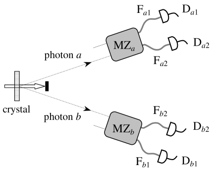
Figure 1: Schematic of the proposed experimental setup. The boxes $\mathrm{MZ}_{a}$ and $\mathrm{MZ}_{b}$ represent the Mach-Zehnder interferometers in the path of the photon $a$ and $b$, respectively. The thick grey lines $\mathrm{F}_{xi}$($x=a,b;\;i=1,2$), represent the single-mode optical fibers. Each of them is coupled with a detector $\mathrm{D}_{xi}$. Other details are given in the text.

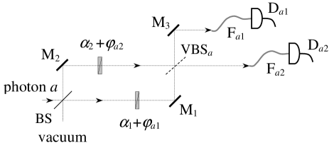
Figure 2: Detailed scheme of the OAM analyzer in the path of the photon $a$. BS denotes a $50/50$ beam splitter, $\mathrm{VBS}_{a}$ a variable-reflectivity beam splitter, $\alpha_{1}$ and $\alpha_{2}$ represent the two SPPs, and $\mathrm{M}_{1},\mathrm{M}_{2},\mathrm{M}_{3}$ represent three ordinary mirrors. The role of $\mathrm{M}_{3}$ is to maintain the input wave function spatially invariant after an even number of reflections. Two additional azimuthal-independent phases $\varphi_{a1}$ and $\varphi_{a2}$ are accounted for.

Figure 3: Schematic drawing of a spiral phase plate (SPP) with a step index ($=$ phase shift per unit angle) $\mathcal{L}=h_{s}(n-n_{0})/\lambda$, where $h_{s}$ is the step height, $n$ and $n_{0}$ are the refractive indices of the SPP and the surrounding medium, respectively, and $\lambda$ is the wavelength of the incident light. In this letter we assume $\mathcal{L}=\ell+1/2,\,\{\ell=1,2,\ldots\}$. The orientation angle $\alpha$ is indicated.

II.1 The spiral phase plates

A spiral phase plate, shown in Fig. 3, is a transparent dielectric plate with an edge dislocation that can be freely rotated around the plate axis Beijersbergen et al. (1994). Let $z$ be the axis of the plate and $\chi$ the rotation angle. When a light beam with transverse profile $\psi(\mathbf{x})$ crosses such a SPP it acquires an azimuthal-dependent phase $\exp(\mathrm{i}f(\chi,\phi))$

$$\psi(\mathbf{x})\rightarrow e^{\mathrm{i}f(\chi,\phi)}\psi(\mathbf{x}),$$ (2)

where

$$e^{\mathrm{i}f(\chi,\phi)}=e^{\mathrm{i}\mathcal{L}(\phi-\chi)}\left[e^{\mathrm{i}2\pi\mathcal{L}}\Theta(\chi-\phi)+\Theta(\phi-\chi)\right].$$ (3)

Here $\mathbf{x}$ is the two-dimensional position vector $\mathbf{x}=(x,y)$ in the transverse plane $z=\mathrm{const.}$, $\phi=\phi(\mathbf{x})$ is the azimuthal angle, and $\mathcal{L}\in\mathbb{R}$ is the phase shift per unit angle. In addition, with $\Theta(X)$ we denoted the Heaviside function which is equal to $1$ for $X>0$ and to zero otherwise. Let $\hat{S}(\chi)$ be the quantum mechanical operator representing the action of a SPP on the arbitrary single-photon state $|\psi\rangle$, and let $|\mathbf{x}\rangle$ denotes the position-representation state of a quasi-monochromatic photon with a given polarization (position state, for short)

$$|\mathbf{x}\rangle=\frac{1}{2\pi}\int\mathrm{d}^{2}\mathbf{q}\,e^{-\mathrm{i}\mathbf{q}\cdot\mathbf{x}}\hat{a}^{\dagger}(\mathbf{q})|0\rangle,$$ (4)

where $\mathbf{q}=(q_{x},q_{y})$ is the transverse photon momentum and $[\hat{a}(\mathbf{q}),\hat{a}^{\dagger}(\mathbf{q}^{\prime})]=\delta^{(2)}(\mathbf{q}-\mathbf{q}^{\prime})$. It is easy to see that the position states $\{|\mathbf{x}\rangle\}$ are orthogonal and form a complete basis in the single-photon Hilbert space

$$\langle\mathbf{x}|\mathbf{x}^{\prime}\rangle = \delta^{(2)}(\mathbf{x}-\mathbf{x}^{\prime}),$$ (5a)

$$\hat{I} = \int\mathrm{d}^{2}\mathbf{x}\,|\mathbf{x}\rangle\langle\mathbf{x}|.$$ (5b)

The quantum operator $\hat{S}(\chi)$ can be determined in analogy with the classical case, by imposing

$$\langle\mathbf{x}|\hat{S}(\chi)|\psi\rangle=e^{\mathrm{i}f(\chi,\phi)}\psi(\mathbf{x}),$$ (6)

and assuming $\psi(\mathbf{x})=\langle\mathbf{x}|\psi\rangle$. Then Eq. (6) can be rewritten as

$$\langle\mathbf{x}|\hat{S}(\chi)|\psi\rangle=e^{\mathrm{i}f(\chi,\phi)}\langle\mathbf{x}|\psi\rangle,$$ (7)

which implies, together with the arbitrariness of $|\psi\rangle$,

$$\langle\mathbf{x}|\hat{S}(\chi)=e^{\mathrm{i}f(\chi,\phi)}\langle\mathbf{x}|.$$ (8)

This equation shows that the SPP operator $\hat{S}(\chi)$ is diagonal in the coordinate basis kets and it is unitary since its eigenvalues $\exp({\mathrm{i}f(\chi,\phi)})$ have modulus $1$. If we multiply both sides of Eq. (8) by $|\mathbf{x}^{\prime}\rangle$, we obtain

$$\begin{array}[]{rcl}\langle\mathbf{x}|\hat{S}(\chi)|\mathbf{x}^{\prime}\rangle&=&e^{\mathrm{i}f(\chi,\phi)}\langle\mathbf{x}|\mathbf{x}^{\prime}\rangle\\ \\ &=&e^{\mathrm{i}f(\chi,\phi^{\prime})}\langle\mathbf{x}|\mathbf{x}^{\prime}\rangle,\end{array}$$ (9)

where the second line of Eq. (9) immediately follows from the orthogonality of the position states. From Eq. (9) we easily obtain

$$\hat{S}(\chi)|\mathbf{x}\rangle=e^{\mathrm{i}f(\chi,\phi)}|\mathbf{x}\rangle,$$ (10)

which shows, together with Eq. (8), that the SPP operator $\hat{S}(\chi)$ is symmetric. From Eq. (10) it is straightforward to write the corresponding transformation law for the spatial creation operators $\hat{a}^{\dagger}(\mathbf{x})$:

$$\hat{S}(\chi)\hat{a}^{\dagger}(\mathbf{x})\hat{S}^{\dagger}(\chi)=e^{\mathrm{i}f(\chi,\phi)}\hat{a}^{\dagger}(\mathbf{x}).$$ (11)

To conclude this paragraph, we define the complementary spiral phase plate, as a SPP that produces a negative azimuthal-dependent phase shift $\exp(-\mathrm{i}f(\chi,\phi))$ on a crossing beam:

$$\psi(\mathbf{x})\rightarrow e^{-\mathrm{i}f(\chi,\phi)}\psi(\mathbf{x}).$$ (12)

Then from the Hermitian-conjugate of Eq. (8) it readily follows that the CSPP is represented by $\hat{S}^{\dagger}(\chi)$.

II.2 The Mach-Zehnder interferometer

Figure 2) shows a detailed scheme of the Mach-Zehnder interferometer $\mathrm{MZ}_{a}$. Photon $a$ enters the Mach-Zehnder through the channel “$1$” and interacts with the first $50/50$ beam splitter. Channel “$2$” is fed with vacuum. A general two-mode single-photon (TMSP) state at the input of $\mathrm{MZ}_{a}$ can be therefore written

$$\begin{array}[]{rcl}\displaystyle{|\psi_{a}\rangle}&=&\displaystyle{\int\mathrm{d}^{2}\mathbf{x}\,\xi(\mathbf{x})\hat{a}_{1}^{\dagger}(\mathbf{x})|0\rangle},\end{array}$$ (13)

where the subscript $1$ denotes the channel $1$. The beam splitter transforms the input TMSP state $|\psi_{a}\rangle$ in a superposition of TMSP states Campos et al. (1989), $|\psi_{a}\rangle\rightarrow|\psi_{a}\rangle_{1}$:

$$\begin{array}[]{rcl}\displaystyle{|\psi_{a}\rangle_{1}}&=&\displaystyle{\hat{U}^{\dagger}|\psi_{a}\rangle}\\ \\ &=&\displaystyle{\int\mathrm{d}^{2}\mathbf{x}\,\xi(\mathbf{x})\hat{U}^{\dagger}\hat{a}_{1}^{\dagger}(\mathbf{x})\hat{U}|0\rangle},\end{array}$$ (14)

where Walborn et al. (2003); Dan

$$\begin{array}[]{rcl}\displaystyle{\hat{U}^{\dagger}\hat{a}_{1}^{\dagger}(\mathbf{x})\hat{U}}&=&\displaystyle{t\hat{a}_{1}^{\dagger}(x,y)-r^{*}\hat{a}_{2}^{\dagger}(x,-y)},\\ \\ \displaystyle{\hat{U}^{\dagger}\hat{a}_{2}^{\dagger}(\mathbf{x})\hat{U}}&=&\displaystyle{r\hat{a}_{1}^{\dagger}(x,-y)+t^{*}\hat{a}_{2}^{\dagger}(x,y)},\end{array}$$ (15)

and we assume $t=1/\sqrt{2},\,r=\mathrm{i}/\sqrt{2}$ for the transmission and reflection coefficients of the $50/50$ beam splitter, respectively. We can then write

$$\begin{array}[]{rcl}\displaystyle{|\psi_{a}\rangle_{1}}&=&\displaystyle{\int\mathrm{d}^{2}\mathbf{x}\,\frac{\xi(\mathbf{x})}{\sqrt{2}}\left[\hat{a}_{1}^{\dagger}(x,y)|0\rangle+\mathrm{i}\hat{a}_{2}^{\dagger}(x,-y)|0\rangle\right]}.\end{array}$$ (16)

The action of the mirror $\mathrm{M}_{2}$ can be described as $\hat{a}_{2}^{\dagger}(x,-y)\rightarrow r\hat{a}_{2}^{\dagger}(x,y)$, where $r=\mathrm{i}$, which causes $|\psi_{a}\rangle_{1}\rightarrow|\psi_{a}\rangle_{2}$, where

$$\begin{array}[]{rcl}\displaystyle{|\psi_{a}\rangle_{2}}&=&\displaystyle{\int\mathrm{d}^{2}\mathbf{x}\,\frac{\xi(\mathbf{x})}{\sqrt{2}}\left[\hat{a}_{1}^{\dagger}(x,y)|0\rangle-\hat{a}_{2}^{\dagger}(x,y)|0\rangle\right]}.\end{array}$$ (17)

After the first beam splitter and the mirror $\mathrm{M}_{2}$, there are two SPPs, one per channel, which perform a unitary operation on the TMSP state: $|\psi_{a}\rangle_{2}\rightarrow|\psi_{a}\rangle_{3}$. Let $\hat{S}(\alpha_{i})$ the operator representing the SPP (CSPP) in the channel $i$ ($i=1,2$). Since under $\hat{S}(\alpha_{i})$, the operators $\hat{a}_{i}^{\dagger}(\mathbf{x})$ transform as

$$\hat{a}_{i}^{\dagger}(\mathbf{x})\rightarrow\hat{S}(\alpha_{i})\hat{a}_{i}^{\dagger}(\mathbf{x})\hat{S}^{\dagger}(\alpha_{i})=e^{\mathrm{i}f{(\alpha_{i},\phi)}}\hat{a}_{i}^{\dagger}(\mathbf{x}),$$ (18)

then the TMSP state after the SPPs can be written as

$${|\psi_{a}\rangle_{3}=\int\mathrm{d}^{2}\mathbf{x}\,\frac{\xi(\mathbf{x})}{\sqrt{2}}\left[e^{\mathrm{i}f(\alpha_{1},\phi)}\hat{a}_{1}^{\dagger}(\mathbf{x})|0\rangle-e^{\mathrm{i}f(\alpha_{2},\phi)}\hat{a}_{2}^{\dagger}(\mathbf{x})|0\rangle\right]},$$ (19)

where Eq. (10) has been used. The action of the mirror $\mathrm{M}_{1}$ can be described as $\hat{a}_{1}^{\dagger}(x,y)\rightarrow-r^{*}\hat{a}_{1}^{\dagger}(x,-y)$, where $r=\mathrm{i}$, which causes $|\psi_{a}\rangle_{3}\rightarrow|\psi_{a}\rangle_{4}$, where

$$\begin{array}[]{rclcl}\displaystyle{|\psi_{a}\rangle_{4}}&=&\displaystyle{\int\mathrm{d}^{2}\mathbf{x}\,\frac{\xi(\mathbf{x})}{\sqrt{2}}}&\displaystyle{\Bigl{[}}&\displaystyle{\mathrm{i}e^{\mathrm{i}f(\alpha_{1},\phi)}\hat{a}_{1}^{\dagger}(x,-y)|0\rangle}\\ &&&&\displaystyle{-e^{\mathrm{i}f(\alpha_{2},\phi)}\hat{a}_{2}^{\dagger}(x,y)|0\rangle\Bigr{]}}.\end{array}$$ (20)

The second beam splitter transforms the creation operators according to Walborn et al. (2003)

$$\begin{array}[]{rcl}\displaystyle{\hat{a}_{1}^{\dagger}(x,-y)}&\rightarrow&\displaystyle{r_{a}\hat{a}_{2}^{\dagger}(x,y)+t_{a}^{*}\hat{a}_{1}^{\dagger}(x,-y)},\\ \\ \displaystyle{\hat{a}_{2}^{\dagger}(x,y)}&\rightarrow&\displaystyle{t_{a}\hat{a}_{2}^{\dagger}(x,y)-r_{a}^{*}\hat{a}_{1}^{\dagger}(x,-y)},\end{array}$$ (21)

where $t_{a}=\cos\theta_{a},\;r_{a}=\mathrm{i}\sin\theta_{a}$. The TMSP state $|\psi_{a}\rangle_{5}$ at the output of the Mach-Zehnder $\mathrm{MZ}_{a}$ can therefore be written as

$$\begin{array}[]{rcl}\displaystyle{|\psi_{a}\rangle_{5}}&=&\displaystyle{\int\mathrm{d}^{2}\mathbf{x}\,\frac{\xi(\mathbf{x})}{\sqrt{2}}\Bigl{\{}\left[\mathrm{i}r_{a}e^{\mathrm{i}f(\alpha_{1},\phi)}-t_{a}e^{\mathrm{i}f(\alpha_{2},\phi)}\right]\hat{a}_{2}^{\dagger}(x,y)}\\ \\ &&\displaystyle{+\left[\mathrm{i}t_{a}^{*}e^{\mathrm{i}f(\alpha_{1},\phi)}+r_{a}^{*}e^{\mathrm{i}f(\alpha_{2},\phi)}\right]\hat{a}_{1}^{\dagger}(x,-y)}\Bigr{\}}|0\rangle.\end{array}$$ (22)

The role of the last mirror $\mathrm{M}_{3}$ is to maintain the initial spatial wave-function $\xi(\mathbf{x})$ invariant; its action can be described as $\hat{a}_{1}^{\dagger}(x,-y)\rightarrow r\hat{a}_{1}^{\dagger}(x,y)$, $(r=\mathrm{i})$, which causes $|\psi_{a}\rangle_{5}\rightarrow|\psi_{a}\rangle_{6}$, where, apart an overall phase factor,

$$\begin{array}[]{rcl}\displaystyle{|\psi_{a}\rangle_{6}}&=&\displaystyle{\int\mathrm{d}^{2}\mathbf{x}\,\frac{\xi(\mathbf{x})}{\sqrt{2}}\Bigl{\{}\left[t_{a}^{*}e^{\mathrm{i}f(\alpha_{1},\phi)}-\mathrm{i}r_{a}^{*}e^{\mathrm{i}f(\alpha_{2},\phi)}\right]\hat{a}_{1}^{\dagger}(x,y)}\\ \\ &&\displaystyle{+\left[-\mathrm{i}r_{a}e^{\mathrm{i}f(\alpha_{1},\phi)}+t_{a}e^{\mathrm{i}f(\alpha_{2},\phi)}\right]\hat{a}_{2}^{\dagger}(x,y)\Bigr{\}}|0\rangle}\\ \\ &=&\displaystyle{\int\mathrm{d}^{2}\mathbf{x}\,\frac{\xi(\mathbf{x})}{\sqrt{2}}\Bigl{\{}}\\ \\ &&\displaystyle{\;\;\;\left[\cos\theta_{a}e^{\mathrm{i}f(\alpha_{1},\phi)}-\sin\theta_{a}e^{\mathrm{i}f(\alpha_{2},\phi)}\right]\hat{a}_{1}^{\dagger}(x,y)}\\ \\ &&\displaystyle{+\left[\sin\theta_{a}e^{\mathrm{i}f(\alpha_{1},\phi)}+\cos\theta_{a}e^{\mathrm{i}f(\alpha_{2},\phi)}\right]\hat{a}_{2}^{\dagger}(x,y)\Bigr{\}}|0\rangle}\\ \\ &\equiv&\displaystyle{\int\mathrm{d}^{2}\mathbf{x}\,\xi(\mathbf{x})\left[A_{1}(\phi)\hat{a}_{1}^{\dagger}(\mathbf{x})+A_{2}(\phi)\hat{a}_{2}^{\dagger}(\mathbf{x})\right]|0\rangle}.\end{array}$$ (23)

Equation (23) shows that for a given $\mathbf{x}$ the TMSP state $|\psi_{a}\rangle_{6}$ spans, as $\theta_{a}$ varies, a two-dimensional space determined by the orthogonal basis $\{\hat{a}_{1}^{\dagger}(\mathbf{x})|0\rangle,\hat{a}_{2}^{\dagger}(\mathbf{x})|0\rangle\}$. In fact, if we define

$$\vec{A}(\phi)=\begin{pmatrix}A_{1}\\ A_{2}\end{pmatrix},\quad\vec{E}(\phi)=\frac{1}{\sqrt{2}}\begin{pmatrix}e^{\mathrm{i}f_{1}}\\ e^{\mathrm{i}f_{2}}\end{pmatrix},$$ (24)

where $f_{i}\equiv f(\alpha_{i},\phi)$, then from Eq. (23) it readily follows

$$\vec{A}(\phi)=\textsf{R}(\theta_{a})\vec{E}(\phi),$$ (25)

where

$$\textsf{R}(\theta_{a})=\begin{pmatrix}\cos\theta_{a}&-\sin\theta_{a}\\ \sin\theta_{a}&\cos\theta_{a}\end{pmatrix},$$ (26)

is the well known $2\times 2$ rotation matrix. Therefore, as $\theta_{a}$ varies from $0$ to $2\pi$, the state $|\psi_{a}\rangle_{6}$ makes a complete rotation in the plane $\{\hat{a}_{1}^{\dagger}(\mathbf{x})|0\rangle,\hat{a}_{2}^{\dagger}(\mathbf{x})|0\rangle\}$. It is easy to see that if we take in account the azimuthal-independent phases $\varphi_{xi}$, the orthogonal matrix $\textsf{R}(\theta_{a})$ must be replaced by the unitary matrix $\textsf{U}(\theta_{a})$ defined as

$$\textsf{U}(\theta_{a})=\begin{pmatrix}e^{\mathrm{i}\varphi_{a1}}\cos\theta_{a}&-e^{\mathrm{i}\varphi_{a2}}\sin\theta_{a}\\ e^{\mathrm{i}\varphi_{a1}}\sin\theta_{a}&e^{\mathrm{i}\varphi_{a2}}\cos\theta_{a}\end{pmatrix},$$ (27)

Now we can repeat for the photon $b$ the very same calculation beginning with the state

$$\begin{array}[]{rcl}\displaystyle{|\psi_{b}\rangle}&=&\displaystyle{\int\mathrm{d}^{2}\mathbf{x}\,\xi(\mathbf{x})\hat{b}_{1}^{\dagger}(\mathbf{x})|0\rangle},\end{array}$$ (28)

at the input of the Mach-Zehnder $\mathrm{MZ}_{b}$ and ending with the state $|\psi_{b}\rangle_{6}$ at the output of $\mathrm{MZ}_{b}$:

$$|\psi_{b}\rangle_{6}=\int\mathrm{d}^{2}\mathbf{x}\,\xi(\mathbf{x})\left[B_{1}(\phi)\hat{b}_{1}^{\dagger}(\mathbf{x})+B_{2}(\phi)\hat{b}_{2}^{\dagger}(\mathbf{x})\right]|0\rangle,$$ (29)

where

$$\begin{array}[]{rcl}\displaystyle{B_{1}(\phi)}&=&\displaystyle{[\cos\theta_{a}e^{-\mathrm{i}f(\beta_{1},\phi)}-\sin\theta_{a}e^{-\mathrm{i}f(\beta_{2},\phi)}]/\sqrt{2}},\\ \\ \displaystyle{B_{2}(\phi)}&=&\displaystyle{[\sin\theta_{a}e^{-\mathrm{i}f(\beta_{1},\phi)}+\cos\theta_{a}e^{-\mathrm{i}f(\beta_{2},\phi)}]/\sqrt{2}}.\end{array}$$ (30)

Note that the minus sign in the exponentials is due to the fact that CSPPs (instead of SPP) are used in the Mach-Zehnder $\mathrm{MZ}_{b}$.

Since the $A_{i}(\phi)$ and $B_{i}(\phi)$ does not depend on the radial coordinate $r=|\mathbf{x}|$, in the following we shall indicate them as $A_{i}(\phi)$ and $B_{i}(\phi)$, respectively.

II.3 The twin-photon state

The OAM-entangled state of a photon pair emitted by a crystal pumped by a $\mathrm{LG}_{0}^{0}$ laser beam, can be written Visser and Nienhuis (2004)

$$|\Psi\rangle\propto\int\mathrm{d}^{2}\mathbf{x}\,\Lambda_{P}(r)\hat{a}^{\dagger}(\mathbf{x})\hat{b}^{\dagger}(\mathbf{x})|0\rangle,$$ (31)

where $\Lambda_{P}(r)\equiv\mathrm{LG}_{0}^{0}(r,w_{P})$ describes the transverse profile of the pump beam, $r=|\mathbf{x}|$, and $w_{P}$ is the beam waist. The state $|\Psi\rangle$ is clearly non-normalizable, therefore we use the symbol “$\propto$” instead of “$=$”. As we shall see, this fact does not represent a problem since all the measurable probabilities will be properly normalized. Passing from the single-mode to the two-mode description introduced in the previous paragraph, we rewrite the two-mode two-photon (TMTP) state $|\Psi\rangle$ as

$$\begin{array}[]{rcl}|\Psi\rangle&\propto&\displaystyle{\int\mathrm{d}^{2}\mathbf{x}\,\Lambda_{P}(r)\hat{a}_{1}^{\dagger}(\mathbf{x})\hat{b}_{1}^{\dagger}(\mathbf{x})|0\rangle}\end{array}$$ (32)

to indicate that both photons enter the channel “1” of their respective interferometers. When the photon pair crosses both the Mach-Zehnder, $|\Psi\rangle$ undergoes the transformation $|\Psi\rangle\rightarrow|\Psi^{\prime}\rangle$:

$$\begin{array}[]{rcl}|\Psi^{\prime}\rangle&\propto&\displaystyle{\int\mathrm{d}^{2}\mathbf{x}\,\Lambda_{P}(r)\Bigl{\{}\left[A_{1}(\phi)\hat{a}_{1}^{\dagger}(\mathbf{x})+A_{2}(\phi)\hat{a}_{2}^{\dagger}(\mathbf{x})\right]|0\rangle}\\ \\ &&\displaystyle{\otimes\left[B_{1}(\phi)\hat{b}_{1}^{\dagger}(\mathbf{x})+B_{2}(\phi)\hat{b}_{2}^{\dagger}(\mathbf{x})\right]|0\rangle\Bigr{\}}}\\ \\ &&\displaystyle{=\sum_{i,j}^{1,2}\int\mathrm{d}^{2}\mathbf{x}\,\Lambda_{P}(r)\Psi_{ij}(\phi)|\mathbf{x}\rangle_{ai}|\mathbf{x}\rangle_{bj}},\end{array}$$ (33)

where $|\mathbf{x}\rangle_{ai}|\mathbf{x}\rangle_{bj}\equiv\hat{a}_{i}^{\dagger}(\mathbf{x})\hat{b}_{j}^{\dagger}(\mathbf{x})|0\rangle$ denotes a position state with the photon $a$ in the channel $i$ and the photon $b$ in the channel $j$, and

$$\Psi_{ij}(\phi)=\varsigma_{ij}A_{i}(\phi)B_{j}(\phi),\qquad(i,j=1,2),$$ (34)

and $\varsigma_{ij}=(3-i-j)+\mathrm{i}(3i+3j-2ij-4)$.

II.4 The single-mode fibers

Figure 2) shows that the output channel $i,\;(i=1,2)$ of each Mach-Zehnder $\mathrm{MZ}_{x},\;(x=a,b)$ is coupled with the single-mode fiber $\mathrm{F}_{xi}$ which sustains the Laguerre-Gaussian mode $\mathrm{LG}_{0}^{0}$ with waist $w_{0}$. For a proper quantum mechanical description of the fiber we need to introduce the Laguerre-Gaussian single-photon states defined as

$$|l,p\rangle=\int\mathrm{d}^{2}\mathbf{x}\,\mathrm{LG}_{p}^{l}(\mathbf{x})|\mathbf{x}\rangle.$$ (35)

From the orthogonality property of the LG functions, it readily follows

$$\begin{array}[]{rcl}\langle l,p|l^{\prime},p^{\prime}\rangle&=&\displaystyle{\int\mathrm{d}^{2}\mathbf{x}\,\left[\mathrm{LG}_{p}^{l}(\mathbf{x})\right]^{*}\mathrm{LG}_{p^{\prime}}^{l^{\prime}}(\mathbf{x})}\\ \\ &=&\displaystyle{\delta_{ll^{\prime}}\delta_{pp^{\prime}}}.\end{array}$$ (36)

When a photon in the arbitrary state $|\xi\rangle$ is coupled to a single-mode fiber, the fiber transforms the input state of the photon in the Laguerre-Gaussian state $|l=0,p=0\rangle\equiv|0,0\rangle$ with probability $|\langle 0,0|\xi\rangle|^{2}$. Since in our scheme the output port of each single-mode fiber is coupled to a detector, the probability $P_{ij}(\theta_{a},\theta_{b})$ that the detector $\mathrm{D}_{ai}$ fires in coincidence with the detector $\mathrm{D}_{bj}$ is given by

$$\begin{array}[]{rcl}\displaystyle{P_{ij}(\theta_{a},\theta_{b})}&\propto&\displaystyle{\left|\int\mathrm{d}^{2}\mathbf{x}\,\Lambda_{P}(r)\Psi_{ij}(\phi)\langle 0,0|\mathbf{x}\rangle_{ai}\langle 0,0|\mathbf{x}\rangle_{bj}\right|^{2}}\\ &&\displaystyle{=\left|\int\mathrm{d}^{2}\mathbf{x}\,\Lambda_{P}(r)\Lambda_{0}^{2}(r)\Psi_{ij}(\phi)\right|^{2}},\end{array}$$ (37)

since $\langle 0,0|\mathbf{x}\rangle_{ai}=\langle 0,0|\mathbf{x}\rangle_{bj}=\langle 0,0|\mathbf{x}\rangle$, and

$$\langle 0,0|\mathbf{x}\rangle=\mathrm{LG}_{0}^{0}(r,w_{0})=\sqrt{\frac{2}{\pi w_{0}^{2}}}e^{-r^{2}/w_{0}^{2}}\equiv\Lambda_{0}(r).$$ (38)

As the $\Psi_{ij}(\phi)$s do not depend on $r$, we can factorize $P_{ij}(\theta_{a},\theta_{b})$ by passing to polar coordinates $(x,y)\rightarrow(r,\phi)$:

$$\begin{array}[]{l}\displaystyle{\int\mathrm{d}^{2}\mathbf{x}\,\Lambda_{P}(r)\Lambda_{0}^{2}(r)\Psi_{ij}(\phi)}\\ \\ \displaystyle{\;\;\;\;\;\;\;\;\;\;=\int_{0}^{\infty}\mathrm{d}r\,r\Lambda_{P}(r)\Lambda_{0}^{2}(r)\int_{0}^{2\pi}\mathrm{d}\phi\Psi_{ij}(\phi)},\end{array}$$ (39)

and cast the radial part aside in order to get

$$P_{ij}(\theta_{a},\theta_{b})\propto\left|\int_{0}^{2\pi}\mathrm{d}\phi\Psi_{ij}(\phi)\right|^{2}.$$ (40)

Finally, from Eqs. (3,22-30) we note that, in practice, the only elementary azimuthal integral one needs to calculate is

$$\begin{array}[]{rcl}\displaystyle{I(\mu,\nu,\mathcal{L})}&=&\displaystyle{\int_{0}^{2\pi}\mathrm{d}\phi e^{\mathrm{i}\left[f(\phi,\mu)-f(\phi,\nu)\right]}}\\ \\ &=&\displaystyle{e^{\mathrm{i}(\mu-\nu)\mathcal{L}}\Bigl{\{}2\pi-\Bigl{[}(1-e^{\mathrm{i}2\pi\mathcal{L}})\Theta(\mu-\nu)}\\ \\ &&\displaystyle{-(1-e^{-\mathrm{i}2\pi\mathcal{L}})\Theta(\nu-\mu)\Bigr{]}(\mu-\nu)\Bigr{\}}},\end{array}$$ (41)

which reduces to the simpler form

$${I(\mu,\nu,l+1/2)}=2\pi e^{-\mathrm{i}(\mu-\nu)(l+1/2)}\left(1-\frac{|\mu-\nu|}{\pi}\right),$$ (42)

for $\mathcal{L}=l+1/2$, where $l\in\{0,1,2,\ldots\}$.

III The Clauser-Horne inequality

In the previous section we calculated directly the coincidence probabilities $P_{ij}(\theta_{a},\theta_{b})$ from the TMTP state $|\Psi^{\prime}\rangle$ at the output of both interferometers. However, to proceed further and test the non-locality of the state $|\Psi^{\prime}\rangle$, we have to specify our scenario more precisely. Let us formalize our experiment as follows. There are two parties, say Alice and Bob, who share the two-photon entangled state $|\Psi\rangle$ given in Eq. (31). Each one of the two entangled photons belong to an $\infty$-dimensional Hilbert space, namely the OAM Hilbert space. Alice and Bob have two distinct measuring apparatuses: $\mathrm{M}_{a}$ and $\mathrm{M}_{b}$ respectively. Each apparatus $\mathrm{M}_{x},\;(x=a,b)$ consists of a two-channel Mach-Zehnder interferometer $\mathrm{MZ}_{x}$, with a parameter $\theta_{x}$ at the experimenter’s disposal, followed by two (one per channel) single-mode fibers $\mathrm{F}_{xi},\;(i=1,2)$. The output ports $i=1,2$ of each $\mathrm{M}_{x}$ are monitored by two detectors $\mathrm{D}_{x1}$ and $\mathrm{D}_{x2}$ respectively. We stress that in this scenario the SPPs rotation angles $\alpha$ and $\beta$ are not experimental “knobs” that can be changed during an experiment. Different pairs $\{\alpha,\beta\}$ define different experiments which use the same initial two-photon entangled state $|\Psi\rangle$. In analogy with the polarization case, Alice can choose between $2$ different measurements, say $A$ and $A^{\prime}$, corresponding to two different choices for the varying-beam-splitter “angles” $\theta_{a}$ and $\theta_{a}^{\prime}$, respectively. Similarly, Bob can choose between $B$ and $B^{\prime}$, corresponding to $\theta_{b}$ and $\theta_{b}^{\prime}$, respectively. Each time Alice and Bob perform a measurement, $\mathrm{M}_{x}$ $(x=a,b)$ gives the string $\{x_{1},x_{2}\}$, where $x_{i}=1$ when the detector $\mathrm{D}_{xi}$ fires and $x_{i}=0$ when it does not. At this point, our scenario is completely defined: We have $2$ parties (Alice and Bob), $2$ measurements ($\theta_{x}$ and $\theta_{x}^{\prime}$) per party, and $2$ possible outcomes ($\{1,0\}$ and $\{0,1\}$) per measurement per party.

Now we can calculate the quantum mechanical predictions for the experimental outcomes. These calculations were already done in the previous paragraph, but here we want to repeat them in a slightly different way in order to display the dichotomic nature of the problem. To begin with, we fix for the rest of this paper, $\alpha_{1}\equiv\alpha,\;\alpha_{2}=\alpha+\pi$ and $\beta_{1}\equiv\beta,\;\beta_{2}=\beta+\pi$. Moreover, we fix $\mathcal{L}=l+1/2$, where $l\in\{0,1,2,\ldots\}$. The TMTP state $|\Psi^{\prime}\rangle$ (33) describes the photon pair at the output the two interferometers, just before the fibers. As shown previously, each fiber projects any input single-photon state in the Laguerre-Gaussian state $|0,0\rangle$. Therefore, from Eq. (33) it readily follows that the two-photon state $|\Psi^{\prime\prime}\rangle$ after the fibers can be written as

$$\begin{array}[]{rcl}|\Psi^{\prime\prime}\rangle&\propto&\displaystyle{\sum_{i,j}^{1,2}|0,0\rangle_{ai}|0,0\rangle_{bj}}\\ \\ &&\displaystyle{\times\int\mathrm{d}^{2}\mathbf{x}\,\Lambda_{P}(r)\Psi_{ij}(\phi)\langle 0,0|\mathbf{x}\rangle_{ai}\langle 0,0|\mathbf{x}\rangle_{bj}}.\end{array}$$ (43)

As was shown in Eq. (39), it is possible to write

$$\begin{array}[]{l}\displaystyle{\int\mathrm{d}^{2}\mathbf{x}\,\Lambda_{P}(r)\Psi_{ij}(\phi)\langle 0,0|\mathbf{x}\rangle_{ai}\langle 0,0|\mathbf{x}\rangle_{bj}}\\ \\ \displaystyle{\;\;\;=\int_{0}^{\infty}\mathrm{d}r\,r\Lambda_{P}(r)\Lambda_{0}^{2}(r)\times\int_{0}^{2\pi}\mathrm{d}\phi\,\Psi_{ij}(\phi)}\\ \\ \displaystyle{\;\;\;\equiv R\times C_{ij}(\theta_{a},\theta_{b})},\end{array}$$ (44)

where the radial integral $R$ does not depend nor on $\alpha$ and $\beta$, nor on $\theta_{a}$ and $\theta_{b}$. We can write then

$$|\Psi^{\prime\prime}\rangle\propto\sum_{i,j}^{1,2}C_{ij}|i,j\rangle,$$ (45)

where $R$ has been absorbed into the proportionality factor and $|i,j\rangle$ is a shorthand for $|0,0\rangle_{ai}|0,0\rangle_{bj}$. At this point, it is straightforward to write the normalized TMTP state $|\Psi_{00}\rangle$ after the fibers as

$$|\Psi_{00}\rangle=\sum_{i,j}^{1,2}\lambda_{ij}|i,j\rangle,$$ (46)

were we have defined the two-photon amplitudes

$$\lambda_{ij}(\theta_{a},\theta_{b})=\frac{\varsigma_{ij}\int_{0}^{2\pi}\mathrm{d}\phi\,A_{i}(\phi)B_{j}(\phi)}{\sqrt{\sum_{i,j}^{1,2}\left|\int_{0}^{2\pi}\mathrm{d}\phi\,A_{i}(\phi)B_{j}(\phi)\right|^{2}}}.$$ (47)

The state $|\Psi_{00}\rangle$ is clearly entangled since the coefficients $\lambda_{ij}$ are, in general, not factorable. Moreover, it belongs to a $4$-dimensional Hilbert space, as a two-photon polarization-entangled state, since the continuous variables $(r,\phi)$ have been integrated out. In fact, all our operations can be summarized in this way: We began with an OAM-entangled two-photon state belonging to an infinite-dimensional Hilbert space $\mathcal{H}_{ab}^{\infty\times\infty}$. Then we performed on this state some unitary operations which permitted us to span a certain sub-space of $\mathcal{H}_{ab}^{\infty\times\infty}$. Finally, we projected the transformed state onto a $4$-dimensional Hilbert space $\mathcal{H}_{ab}^{2\times 2}$, the two dimensions (per photon) being provided by the two spatial modes (“arms”) of the Mach-Zehnder interferometer. In this way the entanglement-preserving mapping $\mathcal{H}_{ab}^{\infty\times\infty}\rightarrow\mathcal{H}_{ab}^{2\times 2}$ was accomplished. We stress that the azimuthal integration in Eq. (47) clearly shows that the final state $|\Psi_{00}\rangle$ is entangled because the initial state $|\Psi\rangle$ from the crystal was entangled, and not because the beam splitters in the MZs created the entanglement Kim et al. (2002).

Now that we have reduced our problem to a $4$-dimensional one, there are several inequalities at our disposal to check the non-locality of the state $|\Psi_{00}\rangle$. The best known are the Bell inequality Bell (1965), the Clauser-Horne-Shimony-Holt (CHSH) inequality Clauser et al. (1969), and the Clauser-Horne (CH) inequality Clauser and Horne (1974). Since we are proposing an experiment, we choose here to check the CH inequality which, differently from the CHSH inequality, does not require the fair sampling hypothesis Garuccio and Rapisarda (1981) to allow the use of unnormalized experimental data. In practice, an experimenter choose a measurement, say $(A,B)$, and repeats it $N$ times ($N$ realizations) obtaining two strings $\{x_{1k},x_{2k}\},\;(x=a,b;\;x_{ik}=0,1)$ for each realization $k,\;(k=1,\ldots,N)$. Then, for $N\gg 1$, the coincidence probabilities $P_{ij}(\theta_{a},\theta_{b})$ are well approximated by the coincidence frequencies $F_{ij}(\theta_{a},\theta_{b})$

$$F_{ij}(\theta_{a},\theta_{b})=\frac{1}{N}\sum_{k=1}^{N}\Theta(a_{ik}b_{jk}-1/2),$$ (48)

where $\Theta$ is the Heaviside step function. These frequencies are clearly not “absolute” since in a real experiment there are always missing outcomes due, for example, to detector inefficiencies and to losses. In other words, we can say that the experimenter has not access to the normalized state $|\Psi_{00}\rangle$, but only to the unnormalized one $|\Psi^{\prime\prime}\rangle$ (45). Therefore, in order write the CH inequality in a useful form for an experimenter, we calculate the following unnormalized coincidences probabilities

$$\displaystyle{P_{ab}(\theta_{a},\theta_{b})} = \displaystyle{p_{11},}$$ (49a)

$$\displaystyle{P_{ab}(\theta_{a},\infty)} = \displaystyle{p_{11}+p_{12},}$$ (49b)

$$\displaystyle{P_{ab}(\infty,\theta_{b})} = \displaystyle{p_{11}+p_{21},}$$ (49c)

$$\displaystyle{P_{ab}(\infty,\infty)} = \displaystyle{p_{11}+p_{12}+p_{21}+p_{22}},$$ (49d)

where $p_{ij}=\left|C_{ij}(\theta_{a},\theta_{b})\right|^{2}$, and define the Bell-Clauser-Horne parameter $S$ as

$$S=\frac{P_{ab}(\theta_{a},\theta_{b})-P_{ab}(\theta_{a},\theta_{b}^{\prime})+P_{ab}(\theta_{a}^{\prime},\theta_{b})+P_{ab}(\theta_{a}^{\prime},\theta_{b}^{\prime})-P_{ab}(\theta_{a}^{\prime},\infty)-P_{ab}(\infty,\theta_{b})}{P_{ab}(\infty,\infty)}.$$ (50)

Then, the CH inequality requires

$$S\leq 0,$$ (51)

for any objective local theory.

From Eq. (49a-49d) it is simple to calculate the four coincidence probabilities: They are explicitly given in Appendix A. They seems complicated but after a careful inspection it is easy to see that if we choose a common orientation $\alpha=\beta$ for the SPPs and the CSPPs for the two photons, they reduce to the simpler form

$$\displaystyle{\frac{P_{ab}(\theta_{a},\theta_{b})}{P_{ab}(\infty,\infty)}} = \displaystyle{\frac{1}{2}\cos^{2}(\theta_{a}-\theta_{b}),}$$ (52a)

$$\displaystyle{\frac{P_{ab}(\theta_{a},\infty)}{P_{ab}(\infty,\infty)}} = \displaystyle{\frac{1}{2},}$$ (52b)

$$\displaystyle{\frac{P_{ab}(\infty,\theta_{b})}{P_{ab}(\infty,\infty)}} = \displaystyle{\frac{1}{2}.}$$ (52c)

With the particular choice of varying-beam-splitter angles

$$\begin{array}[]{lcl}\theta_{a}&=&0,\\ \theta_{a}^{\prime}&=&\pi/4,\\ \theta_{b}&=&\pi/8,\\ \theta_{b}^{\prime}&=&3\pi/8,\end{array}$$

we achieve the maximum violation $S=(\sqrt{2}-1)/2$ of the CH inequality. This result is valid for all pairs of “external” parameters $(\alpha,\beta=\alpha)$.

This is the main result of this paper. Differently from the polarization case, here we have the additional parameter $\alpha$ which can be varied from $0$ to $2\pi$ in order to span part of the infinite-dimensional OAM-entangled two-photon Hilbert space. Different values of $\alpha$ define different experiments and all these experiments give the maximum violation of the CH inequality.

We stress that the condition $\alpha=\beta$ is sufficient but not necessary to obtain high violation of CH inequality in our scheme. In fact, by numerical search, we found many pairs $\alpha\neq\beta$ which produces violations bigger than, e.g., $0.204$.

IV Discussion and conclusions

What is the meaning of the SPP orientation angles pair $(\alpha,\beta)$? In order to answer this question, let us summarize our previous results as follows. Consider a detection event represented by the string $D_{ij}(\theta_{a},\theta_{b})\equiv\{\{a_{1},a_{2}\},\{b_{1},b_{2}\}\}$. It is not difficult to show that the probability $P_{ij}(\theta_{a},\theta_{b})$ of such an event can be written as

$$P_{ij}(\theta_{a},\theta_{b})=\bigl{|}\langle 0,0|\langle 0,0|\hat{U}_{i}(\alpha,\theta_{a})\otimes\hat{U}_{j}^{\dagger}(\beta,\theta_{b})|\Psi^{\mathrm{in}}\rangle\bigr{|}^{2},$$ (53)

where

$$\hat{U}_{i}(\chi,\theta_{x})=\sum_{j=1}^{2}R_{ij}(\theta_{x})\hat{S}(\chi_{j})/\sqrt{2},\,\quad\left\{\begin{array}[]{c}i=1,2,\\ x=a,b,\end{array}\right.$$ (54)

$[\chi_{j}=\chi+(j-1)\pi,\,(\chi=\alpha,\beta)]$ is the operator representing the propagation of a photon through the channel “$i$” of $\mathrm{MZ}_{x}$, and $\hat{S}(\chi_{j})$ is the quantum-mechanical operator representing a SPP oriented at angle $\chi_{j}$ Aie . From Eqs. (43-44) it follows that when the event $D_{ij}(\theta_{a},\theta_{b})$ occurs, the input state $|\Psi^{\mathrm{in}}\rangle$ is projected onto the state $|u_{i}(\alpha,\theta_{a})\rangle|\bar{u}_{j}(\beta,\theta_{b})\rangle$, where

$$\begin{array}[]{rcl}\displaystyle{|u_{i}(\alpha,\theta_{a})\rangle}&=&\displaystyle{\hat{U}_{i}^{\dagger}(\alpha,\theta_{a})|0,0\rangle}\\ &\equiv&\displaystyle{\sum_{j=1}^{2}R_{ij}(\theta_{a})|S(\alpha_{j})\rangle/\sqrt{2}},\end{array}$$ (55)

and $|S(\alpha_{j})\rangle\equiv\hat{S}^{\dagger}(\alpha_{j})|0,0\rangle$. In a similar manner we define $|\bar{u}_{j}(\beta,\theta_{b})\rangle=\hat{U}_{j}(\beta,\theta_{b})|0,0\rangle$ and $|\bar{S}(\beta_{j})\rangle\equiv\hat{S}(\beta_{j})|0,0\rangle$. From $\langle S(\alpha_{i})|S(\alpha_{j})\rangle=\delta_{ij}=\langle\bar{S}(\beta_{i})|\bar{S}(\beta_{j})\rangle$ Sum , it follows that $\{|S(\alpha)\rangle,|S(\alpha+\pi)\rangle\}$ and $\{|\bar{S}(\beta)\rangle,|\bar{S}(\beta+\pi)\rangle\}$ form an orthogonal two-dimensional basis for the photons $a$ and $b$, respectively. Therefore, Eq. (45) tells us that the state $|u_{i}(\alpha,\theta_{a})\rangle|\bar{u}_{j}(\beta,\theta_{b})\rangle$ onto which Alice and Bob project their state $|\Psi^{\mathrm{in}}\rangle$, is confined to the four-dimensional two-photon subspace spanned by the basis $\{|S(\alpha_{i})\rangle\otimes|\bar{S}(\beta_{j})\rangle\},\,(i,j=1,2)$. Moreover, we can see that, e.g., the basis $\{|S(\alpha)\rangle,|S(\alpha+\pi)\rangle\}$ defines a dichotomic subspace as the basis $\{|H\rangle,|V\rangle\}$ does in the polarization space. It is clear then that when we choose a pair $(\alpha,\beta)$ of SPPs orientations, we uniquely fix a four-dimensional two-photon subspace. Since the CH inequalities are applicable to the counts at any pair of detectors which measure dichotomic variables (irrespective of the dimensionality of the bipartite quantum state $|\Psi^{\mathrm{in}}\rangle$ under examination Peres (1978); Żukowski et al. (1997)), we can choose other pairs $(\alpha^{\prime},\beta^{\prime})$ of SPPs orientations (which define other four-dimensional two-photon subspaces), repeat the measurements, and find again the maximum violation of CH inequalities. Now, providing that the state vectors $\{|S(\chi)\rangle,|S(\chi+\pi)\rangle,|S(\chi^{\prime})\rangle,|S(\chi^{\prime}+\pi)\rangle,|S(\chi^{\prime\prime})\rangle,|S(\chi^{\prime\prime}+\pi)\rangle,\dots\}$ ($\chi=\alpha,\beta$) are chosen to be linearly independent, we can extend the CH test to the $N$ pairs $\{(\alpha,\beta),(\alpha^{\prime},\beta^{\prime}),(\alpha^{\prime\prime},\beta^{\prime\prime}),\ldots,(\alpha^{(N)},\beta^{(N)})\}$ defining $N$ pairs of two-dimensional subspaces whose union define a $2N\times 2N$ two-photon subspace. In this way we can demonstrate the non-local nature of the high-dimensional two-photon OAM-entangled states.

In summary, in this paper we proposed a novel experimental setup to investigate the non-locality of high-dimensional two-photon OAM-entangled states generated by SPDC. We use a pair of modified Mach-Zehnder interferometers (one per photon), as OAM analyzers. Inside each MZ there are two SPPs (one per arm) which can rotate around their axes and permit us to explore the infinite-dimensional two-photon Hilbert space. The output port of each MZ is made of a reflectivity-varying beam splitter which acts as a polarizer in the two-dimensional space defined by the two spatial modes (the two arms) of each MZ. When the output ports of these OAM analyzers are fed into single-mode optical fibers, the effective dimensionality of the two-photon Hilbert space reduces from $\infty$ to $4$. Because of this entanglement-preserving dimensional reduction, our experimental scheme permits us to check the non-locality of the two-photon OAM-entangled state, by using a $d\times N_{a}\times N_{b}=2\times 2\times 2$ inequality Massar et al. (2002). In this way we found the maximum violation of the CH inequality for any four-dimensional two-photon subspace selected by the SPPs orientations. Moreover, because of the strict analogy between ours four-dimensional two-photon subspaces and four-dimensional two-photon polarization space, other interesting experiments (e.g. teleportation of spatial degrees of freedom) can be implemented by using our scheme.

Appendix A

For completeness, we give here explicit expressions for the unnormalized probabilities displayed in Eq. (49a-49d). Here $\delta=\alpha-\beta$.

$$\begin{array}[]{rcl}\displaystyle{P_{ab}}\displaystyle{(\theta_{a},\theta_{b})}&=&\displaystyle{\delta^{2}\cos^{2}(\theta_{a}-\theta_{b})-2\pi|\delta|\cos^{2}(\theta_{a}-\theta_{b})}\\ &&\displaystyle{+\sin^{2}\theta_{a}\Bigl{\{}\pi^{2}\sin^{2}\theta_{b}+\cos^{2}\theta_{b}\Bigl{[}2\pi^{2}+\delta^{2}}\\ &&\displaystyle{-2\pi\left(\delta+|\pi-\delta|\right)\Bigr{]}\Bigr{\}}+\cos^{2}\theta_{a}\Bigl{\{}\pi^{2}\cos^{2}\theta_{b}}\\ &&\displaystyle{+\sin^{2}\theta_{b}\Bigl{[}2\pi^{2}+\delta^{2}-2\pi\left(-\delta+|\pi+\delta|\right)\Bigr{]}\Bigr{\}}}\\ &&\displaystyle{+\frac{1}{2}\sin(2\theta_{a})\sin(2\theta_{b})\Bigl{[}\pi\left(|\pi+\delta|+|\pi-\delta|\right)}\\ &&\displaystyle{-|\pi+\delta||\pi-\delta|\Bigr{]},}\end{array}$$ (56)

$$\begin{array}[]{rcl}\displaystyle{P_{ab}(\theta_{a},\infty)}&=&\displaystyle{3\pi^{2}+2\delta^{2}-\pi\Bigl{(}|\pi+\delta|+2|\delta|+|\pi-\delta|\Bigr{)}}\\ &&\displaystyle{+\pi\Bigl{[}2\delta-|\pi+\delta|+|\pi-\delta|\Bigr{]}\cos(2\theta_{a})},\end{array}$$ (57)

$$\begin{array}[]{rcl}\displaystyle{P_{ab}(\infty,\theta_{b})}&=&\displaystyle{3\pi^{2}+2\delta^{2}-\pi\Bigl{(}|\pi+\delta|+2|\delta|+|\pi-\delta|\Bigr{)}}\\ &&\displaystyle{+\pi\Bigl{[}2\delta-|\pi+\delta|+|\pi-\delta|\Bigr{]}\cos(2\theta_{b})},\end{array}$$ (58)

$$P_{ab}(\infty,\infty)=6\pi^{2}+4\delta^{2}-2\pi\Bigl{(}|\pi+\delta|+2|\delta|+|\pi-\delta|\Bigr{)}.$$ (59)

References

- Nielsen and Chuang (2002) M. A. Nielsen and I. L. Chuang, Quantum Computation and Quantum Information (Cambridge University Press, Cambridge, UK, 2002), reprinted first ed.
- Gisin et al. (2002) N. Gisin, G. Ribody, W. Tittel, and H. Zbinden, Rev. Mod. Phys. 74, 145 (2002).
- Kwiat et al. (1995) P. G. Kwiat, K. Mattle, H. Weinfurter, A. Zeilinger, A. V. Sergienko, and Y. Shih, Phys. Rev. Lett. 75, 4337 (1995).
- Mair et al. (2001) A. Mair, A. Vaziri, G. Weihs, and A. Zeilinger, Nature (London) 412, 313 (2001).
- Vaziri et al. (2002) A. Vaziri, G. Weihs, and A. Zeilinger, Phys. Rev. Lett. 89, 240401 (2002).
- de Riedmatten et al. (2002) H. de Riedmatten, I. Marcikic, H. Zbinden, and N. Gisin, Quantum Inf. Comput. 2, 425 (2002).
- Law and Eberly (2004) C. K. Law and J. H. Eberly, Phys. Rev. Lett. 92, 127903 (2004).
- (8) L. Neves, S. Pádua, and C. Saavedra, Phys. Rev. A 69, 042305 (2004); L. Neves, G. Lima, J. G. Aguirre Gómez, C. H. Monken, C. Saavedra, and S. Pádua, Phys. Rev. Lett. 94, 100501 (2005).
- O’Sullivan-Hale et al. (2005) M. N. O’Sullivan-Hale, I. A. Khan, R. W. Boyd, and J. C. Howell, Phys. Rev. Lett. 94, 220501 (2005).
- (10) A. Acín, N. Gisin, L. Masanes, V. Scarani, arXiv:quant-ph/0310166 (2003).
- Oemrawsingh et al. (2004) S. S. R. Oemrawsingh, A. Aiello, E. R. Eliel, G. Nienhuis, and J. P. Woerdman, Phys. Rev. Lett. 92, 217901 (2004).
- (12) S. S. R. Oemrawsingh, X. Ma, D. Voigt, A. Aiello, E. R. Eliel, G. W. ’t Hooft, and J. P. Woerdman, arXiv:quant-ph/0506253.
- Clauser and Horne (1974) J. Clauser and M. A. Horne, Phys. Rev. D 10, 526 (1974).
- Jeffers et al. (1993) J. R. Jeffers, N. Imoto, and R. Loudon, Phys. Rev. A 47, 3346 (1993).
- Beijersbergen et al. (1994) M. W. Beijersbergen, R. P. C. Coerwinkel, M. Kristensen, and J. P. Woerdman, Opt. Commun. 112, 321 (1994).
- Campos et al. (1989) R. A. Campos, B. E. A. Saleh, and M. C. Teich, Phys. Rev. A 40, 1371 (1989).
- Walborn et al. (2003) S. P. Walborn, A. N. de Oliveira, S. Pádua, and C. H. Monken, Phys. Rev. Lett. 90, 143601 (2003).
- (18) Gui-F. Dang, Li-P. Deng, and Kaige Wang, arXiv:quanth-ph/0504057 (2005).
- Visser and Nienhuis (2004) J. Visser and G. Nienhuis, Eur. Phys. J. D 29, 301 (2004).
- Kim et al. (2002) M. S. Kim, W. Son, V. Bužek, and P. L. Knight, Phys. Rev. A 65, 032323 (2002).
- Bell (1965) J. S. Bell, Physics (N.Y.) 1, 195 (1965).
- Clauser et al. (1969) J. F. Clauser, M. A. Horne, A. Shimony, and R. A. Holt, Phys. Rev. Lett. 23, 880 (1969).
- Garuccio and Rapisarda (1981) A. Garuccio and V. A. Rapisarda, Il Nuovo Cimento 65A, 269 (1981).
- (24) A. Aiello, S. S. R. Oemrawsingh, E. R. Eliel, and J. P. Woerdman, arXiv:quant-ph/0503034 (2005).
- (25) S. S. R. Oemrawsingh, A. Aiello, E. R. Eliel, and J. P. Woerdman, arXiv:quant-ph/0401148 (2004).
- Żukowski et al. (1997) M. Żukowski, A. Zeilinger, and M. A. Horne, Phys. Rev. A 55, 2564 (1997).
- Peres (1978) A. Peres, Am. J. Phys. 46, 745 (1978).
- Massar et al. (2002) S. Massar, S. Pironio, J. Roland, and B. Gisin, Phys. Rev. A 66, 052112 (2002).