S-wave quantum entanglement in a harmonic trap

Abstract

We analyze the quantum entanglement between two interacting atoms trapped in a spherical harmonic potential. At ultra-cold temperature, ground state entanglement is generated by the dominated s-wave interaction. Based on a regularized pseudo-potential Hamiltonian, we examine the quantum entanglement by performing the Schmidt decomposition of low-energy eigenfunctions. We indicate how the atoms are paired and quantify the entanglement as a function of a modified s-wave scattering length inside the trap.

I Introduction

The interactions between trapped ultra-cold atoms govern many interesting collective quantum phenomena, ranging from Bose-Einstein condensation Leggett to recently observed fermion superfluid bcs . At sufficiently low energies, it is known that short ranged atom-atom interactions can be replaced by a pointlike regularized pseudo-potential under the shape independent approximation Huang . The strength of such a pseudo-potential is determined by a s-wave scattering length $a$ only, and hence one can control atom-atom interaction by tuning the scattering length via the technique of Feshbach resonance. For trapped systems, the theory of pseudo-potential has been examined in details by several authors Busch ; Block . As long as the range of the actual atom-atom interaction is short compared with the width of the trap, low energy eigenfunctions can be accurately captured by the eigenfunctions of the pseudo-potential, except for a few tightly bound states that may exist inside the range of the inter-atomic potential. Such a universal applicability is the essence of shape independent approximation. Therefore the study of eigenfunctions of pseudo-potentials would provide useful insight about generic features of two-body correlations in the low energy regime.

In this paper, we address a fundamental question of how the scattering length controls quantum correlations between two ultra-cold atoms inside a harmonic trap. Quantum control of trapped ultracold atoms has been a subject of considerable research interest, regarding potential applications in quantum information processing jaksch1 ; jaksch2 . For example, collisions of atoms can be exploited to perform various quantum logic operations jaksch2 . However, the nature of quantum entanglement arising from s-wave scattering has not been fully explored frees . Such an entanglement is inherent in the continuous degree of freedom of atoms, and it may have effects on the fidelity of quantum gates based upon collisional mechanisms jaksch2 . In this paper we will analyze the quantum entanglement of the low energy eigenstates defined by the regularized pseudo-potential and the harmonic trap. By performing the Schmidt decomposition of low energy eigenfunctions, we show that quantum entanglement is manifested as pairing of atoms in a set of orthogonal mode functions in three-dimensional space. In particular, the angular momenta are identified as good quantum numbers to characterize the Schmidt mode functions. We will present numerical results that quantify the degree of entanglement as a function of the scattering length $a$. In addition, we will examine the entanglement in the $a\to\infty$ limit. Such a strong coupling regime corresponds to the unitarity limit in degenerate quantum gases ho . The study of pairing in two-body models in such a limit may shed light on quantum correlations in the more difficult many body problems.

II Regularized Hamiltonian and energy eigenstates

To begin with, we consider a system of two interacting atoms with equal mass trapped in a spherical harmonic potential. The Hamiltonian of the system is given by,

$$H=-\frac{{\hbar^{2}}}{{2m}}\nabla_{1}^{2}-\frac{{\hbar^{2}}}{{2m}}\nabla_{2}^{2}+\frac{1}{2}m\omega^{2}r_{1}^{2}+\frac{1}{2}m\omega^{2}r_{2}^{2}+V({\bf r}_{1}-{\bf r}_{2}),$$ (1)

where ${\bf r}_{1}$ and ${\bf r}_{2}$ are the position vectors of the two atoms, $m$ is the mass of the atom, and $\omega$ is the trap frequency. The interaction between the two atoms is described by the short range potential $V$ which will be replaced by a pseudo-potential in Eq. (3) under the shape independent approximation. For convenience, we separate the Hamiltonian into a center-of-mass part and a relative part, $H=H_{cm}+H_{rel}$ so that

$$H_{cm}=-\frac{1}{8}\nabla_{R}^{2}+2R^{2},$$ (2)

$$H_{rel}=-\frac{1}{2}\nabla_{r}^{2}+\frac{1}{2}r^{2}+2\pi a\delta^{\left(3\right)}\left(\mathbf{r}\right)\frac{\partial}{{\partial r}}r,$$ (3)

with ${\bf R}=({\bf r}_{1}+{\bf r}_{2})/2$ and ${\bf r}={\bf r}_{1}-{\bf r}_{2}$. Here the energy and length are expressed in units of $\hbar\omega$ and $\left({\hbar/\mu\omega}\right)^{1/2}$ (where $\mu=m/2$ is the reduced mass) respectively. The strength of the pseudo-potential is characterized by the modified s-wave scattering length $a$. For a given inter-atomic potential, the precise value of $a$ depends on the trapping potential and it can be determined self-consistently by the methods discussed in Ref. Block . In this paper we will treat $a$ as a parameter of the Hamiltonian.

The s-wave eigen-functions of the $H$ have been solved analytically in Ref. Busch . Given a scattering length, the eigen-energy $E$ of $H_{rel}$ is defined by the solution of:

$$\frac{{\Gamma\left({-E/2-1/4}\right)}}{{2\Gamma\left({-E/2+3/4}\right)}}=a$$ (4)

with $\Gamma$ being the gamma function. The eigenfunctions of $H_{rel}$ with the energy $E$ are given by:

$$\psi_{E}(\mathbf{r})=Ae^{-r^{2}/2}U\left(-E/2+3/4,3/2,r^{2}\right)$$ (5)

where $A$ is a normalization constant, and $U(\alpha,\beta,z)$ is the Kummer’s function Handbook .

In this paper we assume that the center of mass wave function is the ground state of $H_{cm}$, which is a simple gaussian: $\Phi(\mathbf{R})={{2\sqrt{2}}}e^{-2R^{2}}/{{\pi^{3/4}}}$. Combining $\Phi(\mathbf{R})$ with $\psi_{E}(\mathbf{r})$, the two-particle energy eigenfunctions are given by

$$\Psi\left({{\bf r}_{1},{\bf r}_{2}}\right)=\Phi\left(\mathbf{R}\right)\psi_{E}\left(\mathbf{r}\right).$$ (6)

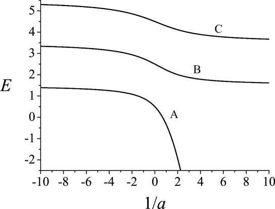
Figure 1: Eigen-energies of $H_{rel}$ as a function of the inverse of dimensionless scaled scattering length. $E$ is in units of $\hbar\omega$. The three branches: A, B, and C correspond to the lowest three states with zero angular momentum (in relative coordinate).

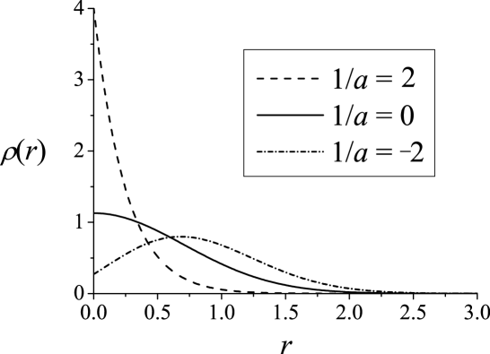
Figure 2: Radial densities $\rho(r)\equiv 4\pi r^{2}|\psi_{E}(r)|^{2}$ associated with the ground state wave functions at $1/a=0,\pm 2$. The radial distance $r$ is in units of $\left({\hbar/\mu\omega}\right)^{1/2}$.

In Fig. 1, we illustrate how the eigen-energies depend on the scattering length. For convenience, we choose to plot with the inverse of scattering length, i.e., $1/a$, in order to indicate the continuous branch associated with the ground states. It should be noted that the ground state energy becomes large and negative when $1/a$ is positive and large. This feature also occurs in the absence of the harmonic trapping potential, and it is due to the existence of a tightly bound state in the $a\to 0^{+}$ limit Busch . As an illustration, we show in Fig. 2 the radial probability density associated with relative coordinate wave functions at several values of $a$.

III Schmidt Decomposition

The characterization of quantum entanglement is achieved by Schmidt decomposition of $\Psi\left({{\bf r}_{1},{\bf r}_{2}}\right)$, which reads:

$$\Psi\left({{\bf r}_{1},{\bf r}_{2}}\right)=\sum\limits_{j}{\sqrt{\lambda_{j}}u_{j}\left({\mathbf{r}_{1}}\right)v_{j}\left({\mathbf{r}_{2}}\right)},$$ (7)

where $\lambda_{j}$ are eigenvalues, and $u_{j}$ and $v_{j}$ are Schmidt eigenmodes defined by,

$$\int\limits{}d{\bf r}_{1}^{\prime}\int\limits{d{\bf r}_{2}}\Psi\left({{\bf r}_{1},{\bf r}_{2}}\right)\Psi^{*}\left({{\bf r}_{1}^{\prime},{\bf r}_{2}}\right)u_{j}({\bf r}_{1}^{\prime})=\lambda_{j}u_{j}({\bf r}_{1}),$$ (8)

$$\int\limits{}d{\bf r}_{2}^{\prime}\int\limits{d{\bf r}_{1}}\Psi\left({{\bf r}_{1},{\bf r}_{2}}\right)\Psi^{*}\left({{\bf r}_{1},{\bf r}_{2}^{\prime}}\right)v_{j}({\bf r}_{2}^{\prime})=\lambda_{j}v_{j}({\bf r}_{2}).$$ (9)

Note that the mode functions $u_{j}$ form a complete and orthonormal set, and the same is true for $v_{j}$. If the atom 1 appears in the mode $u_{j}$, then with certainty the atom 2 must be in the mode $v_{j}$. In other words, Eq. (7) indicates the pairing structure of the two particle state. In addition, the distribution of $\lambda_{j}$ provides a measure of the degree of entanglement. This is usually discussed in terms of the entanglement entropy $S=-\sum\nolimits_{j}{\lambda_{j}}\log\lambda_{j}$. However, a more transparent measure is the effective number of Schmidt modes, which is provided by the Schmidt number: $K\equiv 1/\sum\nolimits_{j}{\lambda_{j}^{2}}$ grobe . A disentangled (product) state corresponds to $K=1$, i.e., there is only one term in the Schmidt decomposition. The larger the value of $K$, the higher the entanglement. We point out that $1/K$ equals the purity of the density matrix of an individual particle. The purity has also been employed as a measure of the degree of entanglement in various physical situations purity .

To carry out the Schmidt decomposition of the wave functions in three dimension, we note that $R=\sqrt{r_{1}^{2}+r_{2}^{2}+2r_{1}r_{2}\cos\gamma}/2$ and $r=\sqrt{r_{1}^{2}+r_{2}^{2}-2r_{1}r_{2}\cos\gamma}$, where $\gamma$ is the angle between $\mathbf{r}_{1}$ and $\mathbf{r}_{2}$. Therefore the wave function $\Psi\left({{\bf r}_{1},{\bf r}_{2}}\right)=\Psi\left({r_{1},r_{2},\cos\gamma}\right)=\sum\limits_{l=0}^{\infty}{\alpha_{l}\left({r_{1},r_{2}}\right)P_{l}\left({\cos\gamma}\right)}$, where $P_{l}(x)$ is the Legendre polynominal, and

$$\alpha_{l}\left({r_{1},r_{2}}\right)=\frac{{2l+1}}{2}\int_{0}^{\pi}{d\gamma\sin\gamma\cdot\Psi\left({r_{1},r_{2},\cos\gamma}\right)P_{l}\left({\cos\gamma}\right)}.$$ (10)

With the help of the addition formula: $(2l+1)P_{l}\left({\cos\gamma}\right)=4\pi\sum\limits_{m=-l}^{l}{Y_{lm}^{*}\left({\theta_{1},\phi_{1}}\right)Y_{lm}\left({\theta_{2},\phi_{2}}\right)}$, we have

$$\Psi({\bf r}_{1},{\bf r}_{2})=4\pi\sum\limits_{l=0}^{\infty}\sum\limits_{m=-l}^{l}{\frac{\alpha_{l}\left({r_{1},r_{2}}\right)}{2l+1}Y^{*}_{lm}\left({\theta_{1},\phi_{1}}\right)Y_{lm}\left({\theta_{2},\phi_{2}}\right)}.$$ (11)

This expression is already partially in the Schmidt form, because the pairing of angular functions has been identified. The remaining task is to decompose $\alpha_{l}\left({r_{1},r_{2}}\right)$ for each $l$. This can be achieved by performing the Schmidt decomposition of the function $r_{1}r_{2}\alpha_{l}(r_{1},r_{2})$, i.e.,

$$r_{1}r_{2}\alpha_{l}\left({r_{1},r_{2}}\right)=\sum\limits_{n}{\sqrt{\lambda_{nl}}u_{nl}\left({r_{1}}\right)v_{nl}\left({r_{2}}\right)}.$$ (12)

Here the prefactor $r_{1}r_{2}$ is introduced in order to ensure correct normalization in radial directions.

The final form of the Schmidt decomposition of the wave function Eq. (5) now reads:

$$\Psi\left({{\bf r}_{1},{\bf r}_{2}}\right)=\sum\limits_{n=1}^{\infty}{\sum\limits_{l=0}^{\infty}{\sum\limits_{m=-l}^{l}{\left({\frac{{4\pi\sqrt{\lambda_{nl}}}}{{2l+1}}}\right)}}}\left[{\frac{{u_{nl}(r_{1})}}{{r_{1}}}Y_{lm}^{*}\left({\theta_{1},\phi_{1}}\right)}\right]\left[{\frac{{v_{nl}(r_{2})}}{{r_{2}}}Y_{lm}\left({\theta_{2},\phi_{2}}\right)}\right].$$ (13)

Our derivation indicates a general feature that for any wave function that is a function of distances $R$ and $r$ only, the angular parts of Schmidt modes are simply the spherical harmonics. The pairing involves angular momentum quantum numbers $(l,m)$ and $(l,-m)$, i.e., the same $l$ and opposite $m$ must be paired. In addition, each $m$ is of equal weight for a given $l$. Therefore if one could select Schmidt modes with a fixed $n$ and $l$ via projective measurement, then the resulting state is a maximally entangled state among various $m$’s on the projected $l$ manifold.

IV Numerical Results

The fact that the angular parts of Schmidt modes can be obtained analytically reduces the computational difficulty in the original three-dimensional problem. Finding $u_{nl}$, $v_{nl}$ and $\lambda_{nl}$ in Eq. (12) is a relatively simple numerical task, because $r_{1}r_{2}\alpha_{l}(r_{1},r_{2})$ behaves as a two-particle (one dimensional) wave function in non-negative $r_{1}$ and $r_{2}$ regions. Specifically, we first obtain $\alpha_{l}(r_{1},r_{2})$ by performing numerical integration of (10) for discretized values of $r_{1}$ and $r_{2}$, typically with the spacing $\Delta r=0.01$. For the s-wave eigenfunctions considered here, it is sufficient to choose $r_{1}$ and $r_{2}$ ranging from $0$ to $3.5$, where the wave functions are mainly confined. Because of the symmetry properties of $r_{1}r_{2}\alpha_{l}(r_{1},r_{2})$, $u_{nl}$ and $v_{nl}$ are the same real functions. Therefore $u_{nl}$, $v_{nl}$ and $\lambda_{nl}$ can be obtained by diagonalizing the matrix $r_{1}r_{2}\alpha_{l}(r_{1},r_{2})$. For low energy states considered in this paper, $l$ up to 30 are typically sufficient in order to obtain convergent results.

We can now obtain the value of $K$ for the state (13) from the Schmidt eigenvalues, i.e.,

$$K=1/\sum\limits_{n=1}^{\infty}{\sum\limits_{l=0}^{\infty}{{\Lambda_{nl}^{2}}}}.$$ (14)

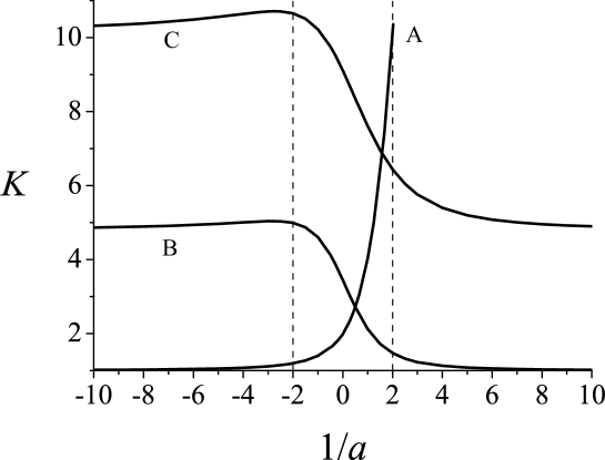
Figure 3: Schmidt number as a function of the inverse of dimensionless scaled scattering length for the low eigenstates associated with the three energy curves in Fig. 1. $K$ is plotted up to $1/a=2$ for the ground state curve A because the high values of $K$ is out of the range of the figure for $1/a>2$.

Here $\Lambda_{nl}=16\pi^{2}\lambda_{nl}/(2l+1)^{3/2}$ is defined. The main result of this paper is shown in Fig. 3, where the values of $K$ are displayed as a function of the inverse of the scaled scattering length for low energy states. We notice that higher excited states generally have higher quantum entanglement. However, the ground state (curve A) shows a distinct behavior in the positive $1/a$ region, where we notice a sharp rise of $K$ as $1/a$ increases.

The strong ground state entanglement in the large positive $1/a$ limit is understood as the appearance of increasingly bounded atoms. This is implied in the ground state energy curve (A) in Fig. 1, as well as in the wave function $(1/a=2)$ shown in Fig. 2. A crude estimation of $K$ can be made from the analytical results of gaussian functions. For gaussian functions separable in the center of mass and relative coordinates, it is known that $K\propto(\Delta R)^{3}/(\Delta r)^{3}$ when the center of mass width $\Delta R$ is much wider than the width of the relative coordinate $\Delta r$ fedorov . Here the tightly bound state corresponds to a strong localization in particle’s relative distance, with $\Delta r$ of order $a$ in the $1/a\gg 1$ limit. Therefore $\Delta R/\Delta r\gg 1$, and hence high values of $K$ can be expected as in the case of gaussians functions. However, we remark that gaussian can only serve as a guide here, because the singular $1/r$ dependence in $\psi_{E}(r)$ cannot be captured by gaussians. Indeed, $K$ depends on $a$ in a complicated form according to our numerical calculations.

For excited eigenstates on the branches B and C, we see an interesting feature in Fig. 3 that the change of quantum entanglement is only sensitive to a range of scaled scattering lengths. Such a window of scaled scattering lengths is highlighted by dash lines in Fig. 3, where we found that $K$ changes significantly with $1/a$ when $1/|a|<2$. Recalling that we are using the length unit defined by the harmonic trap, our results suggest that the s-wave interaction can appreciably affect quantum entanglement in excited states when $a$ is greater than or comparable with the width of a ground state particle inside the trap, i.e., $|a|>\left({\hbar/2m\omega}\right)^{1/2}$. This feature is also true for the ground state with negative scattering lengths.

The structure of quantum entanglement is characterized by the distribution of Schmidt eigenvalues and the Schmidt mode functions. In Fig. 4 we show the distribution $\Lambda_{nl}$ for the ground state with $1/a=-2$ and $1/a=2$. In the case of $1/a=-2$, the entanglement $K=1.2$ is not high because of the presence of a dominant $(n,l,m)=(1,0,0)$ Schmidt mode, which covers about $70\%$ probability of the state. On the contrary, $K=10.13$ is much higher for the $1/a=2$ case. This is shown in the distribution of $\Lambda_{nl}$ (Fig. 5b) in which Schmidt modes with $n=1$ and higher angular momentum number $l$ are involved. In other words, the strong entanglement is mainly manifested in the angular variables.

In Fig. 5, we illustrate the shape of leading Schmidt modes corresponding to the ground state wave functions in Fig. 4. Since the angular part are simple spherical harmonic functions, we show only the radial mode functions in the figure. Apart from the fact that Schmidt modes of positive scattering lengths are more attracted to the origin, the change of scattering length has small effects on the mode functions. This is in contrast to the Schmidt eigenvalues, which are more sensitive to the values of $a$ as depicted in Fig. 4.

Finally, let us discuss the limit of $|a|\to\infty$ or $1/|a|\to 0$. In such a limit, we find that the eigenfunctions take simple analytic forms. We present some of the s-wave eigenfunctions of $H$ in the limit $|a|\to\infty$:

$$\Psi_{10}\left({{\bf r}_{1},{\bf r}_{2}}\right)=\frac{{2}}{{\pi^{3/2}}}\frac{{e^{-r_{1}^{2}}e^{-r_{2}^{2}}}}{{\left|{{\bf r}_{1}-{\bf r}_{2}}\right|}},$$ (15)

$$\Psi_{11}\left({{\bf r}_{1},{\bf r}_{2}}\right)=\frac{{\sqrt{2}}}{{\pi^{3/2}}}\frac{{e^{-r_{1}^{2}}e^{-r_{2}^{2}}}}{{\left|{{\bf r}_{1}-{\bf r}_{2}}\right|}}\left[{1-\left({{\bf r}_{1}-{\bf r}_{2}}\right)^{2}}\right],$$ (16)

$$\Psi_{12}\left({{\bf r}_{1},{\bf r}_{2}}\right)=\frac{{\sqrt{3/2}}}{{\pi^{3/2}}}\frac{{e^{-r_{1}^{2}}e^{-r_{2}^{2}}}}{{\left|{{\bf r}_{1}-{\bf r}_{2}}\right|}}\left[{1-4\left({{\bf r}_{1}-{\bf r}_{2}}\right)^{2}+\frac{4}{3}\left({{\bf r}_{1}-{\bf r}_{2}}\right)^{4}}\right].$$ (17)

Here Eqs. (15-17) correspond to the energy eigenfunctions (center of mass $+$ relative coordinates) associated with the lowest three states of $H_{rel}$, and the ground state of $H_{cm}$. Although Eqs. (15-17) are simple expressions, the Schmidt decomposition still cannot be carried out analytically. We perform numerical calculations which give: $K_{10}=1.98$, $K_{11}=3.45$, and $K_{12}=9.11$ for the wave functions given in Eqs. (15-17). Therefore the degree of entanglement remains finite at the infinite scattering limit.

We remark that the regularized pseudo-potential method can only describe wave functions at inter-atomic distance much larger than the range of the actual inter-atomic potential $b$, i.e., $|{\bf r}_{1}-{\bf r}_{2}|\gg b$. Inside the interaction range $b$, the actual wave functions remain finite as $|{\bf r}_{1}-{\bf r}_{2}|\to 0$. Therefore the singular behavior at ${\bf r}_{1}={\bf r}_{2}$ in Eqs. (15-17) is only an artifact of the shape independent approximation, and hence these wave functions should be understood for $|{\bf r}_{1}-{\bf r}_{2}|\gg b$ only. However, since $b$ is typically much smaller than $\left({\hbar/\mu\omega}\right)^{1/2}$ (which is about the width of $\Psi$), the probability of finding the two particles within the range $b$ is negligible number . This justifies the use of the shape independent approximation here.

V Summary

To summarize, we present a procedure to analyze the s-wave quantum entanglement between two ultra-cold atoms in a spherical harmonic trap. The s-wave interaction is described by the regularized pseudo-potential. By performing the Schmidt decomposition of low energy eigenstates, we quantify the quantum entanglement and indicate its dependence on the modified scattering length. In particular, our Schmidt analysis reveals the angular correlations by showing explicitly the pairing of spherical harmonic functions. For small and positive $a$, the ground states are highly entangled states, and we explain this feature as a consequence of tight binding between the atoms. For low excited states and ground states with negative $a$, we find that the atom-atom interaction can only appreciably affect the entanglement when the scattering length is larger than the width of the (non-interacting) ground state defined by the trap. However, the degree of entanglement remains finite in the large scattering length limit. Our work here indicates that quantum entanglement can be controlled by the scattering length. To explore applications of s-wave entanglement, one may need to establish schemes for detecting Schmidt modes. In addition, the dynamics of entanglement associated with non-stationary states of the system is also an interesting topic for open future investigations.

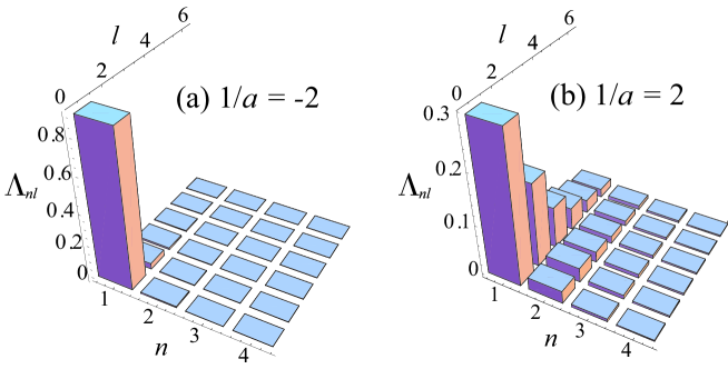
Figure 4: (Color online) Distribution of $\Lambda_{nl}$ (see text) of ground states for: (a) $1/a=-2$ and (b) $1/a=2$.

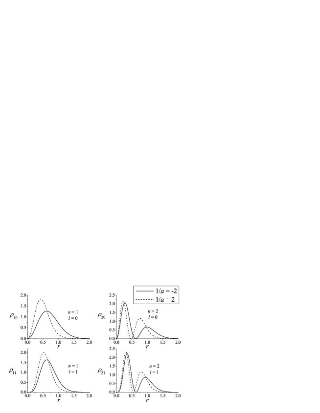
Figure 5: Probability density of the radial part of Schmidt modes $\rho_{nl}=\left|{u_{nl}}\right|^{2}$, where the $u_{nl}$ is defined in Eq. (12). The solid line corresponds to the ground state with $1/a=-2$, while the dash line corresponds to $1/a=2$. The radial distance $r$ is in units of $\left({\hbar/\mu\omega}\right)^{1/2}$.

- (1) For a review see, Anthony J. Leggett, Rev. Mod. Phys. 73, (2001).
- (2) For an overview see, T. L. Ho, Science, 305, 1114 (2004).
- (3) K. Huang, Statistical Mechanics (Wiley, New York 1987).
- (4) T. Busch, B. G. Englert, K. Rzazewski, and M. Wilkens, Found. Phys. 28, 549 (1998).
- (5) M. Block and M. Holthaus, Phys. Rev. A 65, 052102 (2002); E. Tiesinga, C. J. Williams, F. H. Mies, and P. S. Julienne, Phys. Rev. A 61, 063416 (2000); E. L. Bolda, E. Tiesinga, and P. S. Julienne, Phys. Rev. A 66, 013403 (2002).
- (6) D. Jaksch, H.-J. Briegel, J. I. Cirac, C. W. Gardiner, and P. Zoller, Phys. Rev. Lett. 82, 1975 (1999); U. Dorner, P. Fedichev, D. Jaksch, M. Lewenstein, and P. Zoller, Phys. Rev. Lett. 91, 073601 (2003).
- (7) T. Calarco, E. A. Hinds, D. Jaksch, J. Schmiedmayer, J. I. Cirac, and P. Zoller, Phys. Rev. A 61, 022304 (2000); G. K. Brennen, I. H. Deutsch, and C. J. Williams, Phys. Rev. A 65, 022313 (2002).
- (8) The problem of entanglement generation in free space scattering processes was recently addressed by: C. K. Law, Phys. Rev. A 70, 062311 (2004); A. Tal and G. Kurizki, Phys. Rev. Lett. 94, 160503 (2005).
- (9) T.-L. Ho, Phys. Rev. Lett. 92, 090402 (2004).
- (10) R. Grobe, K. Rza̧żewski and J. H. Eberly, J. Phys. B 27, L503 (1994); W.-C. Liu, J. H. Eberly, S. L. Haan and R. Grobe, Phys. Rev. Lett. 83, 520 (1999); R. E. Wagner, P. J. Peverly, Q. Su, and R. Grobe, Laser Phys. 11, 221 (2001); C. K. Law and J. H. Eberly, Phys. Rev. Lett. 92, 127903 (2004); P. Krekora, Q. Su, and R. Grobe, J. Mod. Opt. 52, 489 (2005).
- (11) Ph. Jacquod, Phys. Rev. Lett. 92, 150403 (2004).
- (12) M. Abramowitz and I. A. Stegun, eds., Handbook of Mathematical Functions (Dover, New York, 1972).
- (13) For example, the lowest order van der Waals interaction has a characteristic range of the order of 50Å, and the width of typical trap of frequency 100 Hz is of order 1 m.
- (14) K. W. Chan, J. H. Eberly, quant-ph/0404093; M. V. Fedorov, M. A. Efremov, A. E. Kazakov, K. W. Chan, C. K. Law, and J. H. Eberly, Phys. Rev. A 69, 052117 (2004).