Practical Decoy State for Quantum Key Distribution

Abstract

Decoy states have recently been proposed as a useful method for substantially improving the performance of quantum key distribution. Here, we present a general theory of the decoy state protocol based on only two decoy states and one signal state. We perform optimization on the choice of intensities of the two decoy states and the signal state. Our result shows that a decoy state protocol with only two types of decoy states—-the vacuum and a weak decoy state—asymptotically approaches the theoretical limit of the most general type of decoy state protocols (with an infinite number of decoy states). We also present a one-decoy-state protocol. Moreover, we provide estimations on the effects of statistical fluctuations and suggest that, even for long distance (larger than 100km) QKD, our two-decoy-state protocol can be implemented with only a few hours of experimental data. In conclusion, decoy state quantum key distribution is highly practical.

1 Introduction

The goal of quantum key distribution (QKD) [1] is to allow two distant parties, Alice and Bob, to share a common string of secret (known as the key), in the presence of an eavesdropper, Eve. Unlike conventional cryptography, QKD promises perfect security based on the fundamental laws of physics. Proving the unconditional security of QKD is a hard problem. Fortunately, this problem has recently been solved [2, 3]. See also [4]. Experimental QKD has been successfully demonstrated over 100km of commercial Telecom fibers [5, 6] and commercial QKD systems are already on the market. The most important question of QKD is its security. Real-life QKD systems are often based on attenuated laser pulses (i.e., weak coherent states), which occasionally give out more than one photon. This opens up the possibility of sophisticated eavesdropping attacks such as a photon number splitting attack, where Eve stops all single-photon signals and splits multi-photon signals, keeping one copy herself and re-sending the rest to Bob. The security of practical QKD systems has previously been discussed in [7].

Hwang [8] proposed the decoy state method as an important weapon to combat those sophisticated attack: by preparing and testing the transmission properties of some decoy states, Alice and Bob are in a much better position to catch an eavesdropper. Hwang specifically proposed to use a decoy state with an average number of photon of order $1$. Hwang’s idea was highly innovative. However, his security analysis was heuristic.

In [9], we presented a rigorous security analysis of the decoy state idea. More specifically, we combined the idea of the entanglement distillation approach in GLLP[7] with the decoy method and achieved a formula for key generation rate

$$R\geq q\{-Q_{\mu}f(E_{\mu})H_{2}(E_{\mu})+Q_{1}[1-H_{2}(e_{1})]\},$$ (1)

where $q$ depends on the implementation (1/2 for the BB84 protocol due to the fact that half of the time Alice and Bob disagree with the bases, and if one uses the efficient BB84 protocol [10], $q\approx 1$), the subscript $\mu$ denotes the intensity of signal states, $Q_{\mu}$ is the gain [11] of signal states, $E_{\mu}$ is the overall quantum bit error rate (QBER), $Q_{1}$ is the gain of single photon states, $e_{1}$ is the error rate of single photon states, $f(x)$ is the bi-direction error correction efficiency (See, for example, [12].) as a function of error rate, normally $f(x)\geq 1$ with Shannon limit $f(x)=1$, and $H_{2}(x)$ is binary Shannon information function, given by,

$$H_{2}(x)=-x\log_{2}(x)-(1-x)\log_{2}(1-x).$$

Four key variables are needed in Eq. (1). $Q_{\mu}$ and $E_{\mu}$ can be measured directly from the experiment. Therefore, in the paper [9], we showed rigorously how one can, using the decoy state idea to estimate $Q_{1}$ and $e_{1}$, thus achieving the unconditional security of QKD with the key generation rate given by Eq. (1). Moreover, using the experimental parameters from a particular QKD experiment (GYS) [5], we showed that decoy state QKD can be secure over 140km of Telecom fibers. In summary, we showed clearly that decoy state can indeed substantially increase both the distance and the key generation rate of QKD.

For practical implementations, we [9] also emphasized that only a few decoy states will be sufficient. This is so because contributions from states with large photon numbers are negligible in comparison with those from small photon numbers. In particular, we proposed a Vacuum+Weak decoy state protocol. That is to say, there are two decoy states—a vacuum and a weak decoy state. Moreover, the signal state is chosen to be of order $1$ photon on average. The vacuum state is particularly useful for estimating the background detection rate. Intuitively, a weak decoy state allows us to lower bound $Q_{1}$ and upper bound $e_{1}$.

Subsequently, the security of our Vacuum+ Weak decoy state protocol has been analyzed by Wang [13]. Let us denote the intensities of the signal state and the non-trivial decoy state by $\mu$ and $\mu^{\prime}$ respectively. Wang derived a useful upper bound for $\Delta$:

$$\Delta\leq\frac{\mu}{\mu^{\prime}-\mu}(\frac{\mu e^{-\mu}Q_{\mu^{\prime}}}{\mu^{\prime}e^{-\mu^{\prime}}Q_{\mu}}-1)+\frac{\mu e^{-\mu}Y_{0}}{\mu^{\prime}Q_{\mu}},$$ (2)

where $\Delta$ is the proportion of “tagged” states in the sifted key as defined in GLLP [7]. Whereas we [9] considered a strong version of GLLP result noted in Eq. (1), Wang proposed to use a weak version of GLLP result:

$$R\geq qQ_{\mu}\{-H_{2}(E_{\mu})+(1-\Delta)[1-H_{2}(\frac{E_{\mu}}{1-\Delta})]\}.$$ (3)

Such a weak version of GLLP result does not require an estimation of $e_{1}$. So, it has the advantage that the estimation process is simple. However, it leads to lower values of the key generation rates and distances. The issue of statistical fluctuations in decoy state QKD was also mentioned in [13].

Our observation [9] that only a few decoy states are sufficient for practical implementations has been studied further and confirmed in a recent paper [14], which is roughly concurrent to the present work.

The main goal of this paper is to analyze the security of a rather general class of two-decoy-state protocols with two weak decoy states and one signal state. Our main contributions are as follows. First, we derive a general theory for a decoy state protocol with two weak decoy states. Whereas Wang [13] considered only our Vacuum+Weak decoy state protocol[9] (i.e., a protocol with two decoy states—the vacuum and a weak coherent state), our analysis here is more general. Our decoy method applies even when both decoy states are non-vacuum. Note that, in practice, it may be difficult to prepare a vacuum decoy state. For instance, standard VOAs (variable optical attenuators) cannot block optical signals completely. For the special case of the Vacuum+Weak decoy state protocol, our result generalizes the work of Wang [13].

Second, we perform an optimization of the key generation rate in Eq. (1) as a function of the intensities of the two decoy states and the signal state. Up till now, such an optimization problem has been a key unresolved problem in the subject. We solve this problem analytically by showing that the key generation rate given by Eq. (1) is optimized when both decoy states are weak. In fact, in the limit that both decoy states are infinitesimally weak, we match the best lower bound on $Y_{1}$ and upper bound of $e_{1}$ in the most general decoy state theory where an infinite number of decoy states are used. Therefore, asymptotically, there is no obvious advantage in using more than two decoy states.

Third, for practical applications, we study the correction terms to the key generation rate when the intensities of the two decoy states are non-zero. We see that the correction terms (to the asymptotically zero intensity case) are reasonably small. For the case where one of the two decoy states is a vacuum (i.e., $v_{2}=0$), the correction term remains modest even when the intensity of the second decoy state, $\nu_{1}$ is as high as $25\%$ of that of the signal state.

Fourth, following [13], we discuss the issue of statistical fluctuations due to a finite data size in real-life experiments. We provide a rough estimation on the effects of statistical fluctuations in practical implementations. Using a recent experiment [5] as an example, we estimate that, our weak decoy state proposal with two decoy states (a vacuum and a weak decoy state of strength $\nu$) can achieve secure QKD over more than 100km with only a few hours of experiments. A caveat of our investigation is that we have not considered the fluctuations in the intensities of Alice’s laser pulses (i.e., the values of $\mu,\nu_{1}$ and $\nu_{2}$). This is mainly because of a lack of reliable experimental data. In summary, our result demonstrates that our two-decoy-state proposal is highly practical.

Fifth, we also present a one-decoy-state protocol. Such a protocol has an advantage of being simple to implement, but gives a lower key generation rate. Indeed, we have recently demonstrated experimentally our one-decoy-state protocol over 15km [15]. This demonstrates that one-decoy-state is, in fact, sufficient for many practical applications. In summary, decoy state QKD is simple and cheap to implement and it is, therefore, ready for immediate commercialization.

We remark on passing that a different approach (based on strong reference pulse) to making another protocol (B92 protocol) unconditionally secure over a long distance has recently been proposed in a theoretical paper by Koashi [16].

The organization of this paper is as follows. In section 2, we model an optical fiber based QKD set-up. In section 3, we first give a general theory for $m$ decoy states. We then propose our practical decoy method with two decoy states. Besides, we optimize our choice of the average photon numbers $\mu$ of the signal state and, $\nu_{1}$ and $\nu_{2}$ of the decoy states by maximizing the key generation rate with the experimental parameters in a specific QKD experiment (GYS) [5]. Furthermore, we also present a simple one-decoy-state protocol. In section 4, we discuss the effects of statistical fluctuations in the two-decoy-state method for a finite data size (i.e., the number of pulses transmitted by Alice). Finally, in section 5, we present some concluding remarks.

2 Model

In order to describe a real-world QKD system, we need to model the source, channel and detector. Here we consider a widely used fiber based set-up model [17].

Source: The laser source can be modeled as a weak coherent state. Assuming that the phase of each pulse is totally randomized, the photon number of each pulse follows a Poisson distribution with a parameter $\mu$ as its expected photon number set by Alice. Thus, the density matrix of the state emitted by Alice is given by

$$\rho_{A}=\sum^{\infty}_{i=0}\frac{\mu^{i}}{i!}\,e^{-\mu}\,|i\rangle\langle i|,$$ (4)

where $|0\rangle\langle 0|$ is vacuum state and $|i\rangle\langle i|$ is the density matrix of i-photon state for $i=1,2\cdots$.

Channel: For optical fiber based QKD system, the losses in the quantum channel can be derived from the loss coefficient $\alpha$ measured in dB/km and the length of the fiber $l$ in km. The channel transmittance $t_{AB}$ can be expressed as

$$t_{AB}=10^{-\frac{\alpha l}{10}}.$$

Detector: Let $\eta_{Bob}$ denote for the transmittance in Bob’s side, including the internal transmittance of optical components $t_{Bob}$ and detector efficiency $\eta_{D}$,

$$\eta_{Bob}=t_{Bob}\eta_{D}.$$

Then the overall transmission and detection efficiency between Alice and Bob $\eta$ is given by

$$\eta=t_{AB}\eta_{Bob}.$$ (5)

It is common to consider a threshold detector in Bob’s side. That is to say, we assume that Bob’s detector can tell a vacuum from a non-vacuum state. However, it cannot tell the actual photon number in the received signal, if it contains at least one photon.

It is reasonable to assume the independence between the behaviors of the $i$ photons in i-photon states. Therefore the transmittance of i-photon state $\eta_{i}$ with respect to a threshold detector is given by

$$\eta_{i}=1-(1-\eta)^{i}$$ (6)

for $i=0,1,2,\cdots$.

Yield: define $Y_{i}$ to be the yield of an i-photon state, i.e., the conditional probability of a detection event at Bob’s side given that Alice sends out an i-photon state. Note that $Y_{0}$ is the background rate which includes the detector dark count and other background contributions such as the stray light from timing pulses.

The yield of i-photon states $Y_{i}$ mainly come from two parts, background and true signal. Assuming that the background counts are independent of the signal photon detection, then $Y_{i}$ is given by

$$Y_{i} =Y_{0}+\eta_{i}-Y_{0}\eta_{i}$$ (7)

$$\cong Y_{0}+\eta_{i}.$$

Here we assume $Y_{0}$ (typically $10^{-5}$) and $\eta$ (typically $10^{-3}$) are small.

The gain of i-photon states $Q_{i}$ is given by

$$Q_{i} =Y_{i}\frac{\mu^{i}}{i!}e^{-\mu}.$$ (8)

The gain $Q_{i}$ is the product of the probability of Alice sending out an $i$-photon state (follows Poisson distribution) and the conditional probability of Alice’s $i$-photon state (and background) will lead to a detection event in Bob.

Quantum Bit Error Rate: The error rate of i-photon states $e_{i}$ is given by

$$e_{i}=\frac{e_{0}Y_{0}+e_{detector}\eta_{i}}{Y_{i}}$$ (9)

where $e_{detector}$ is the probability that a photon hit the erroneous detector. $e_{detector}$ characterizes the alignment and stability of the optical system. Experimentally, even at distances as long as 122km, $e_{detector}$ is more or less independent of the distance. In what follows, we will assume that $e_{detector}$ is a constant. We will assume that the background is random. Thus the error rate of the background is $e_{0}=\frac{1}{2}$. Note that Eqs. (6), (7), (8) and (9) are satisfied for all $i=0,1,2,\cdots$.

The overall gain is given by

$$Q_{\mu} =\sum_{i=0}^{\infty}Y_{i}\frac{\mu^{i}}{i!}e^{-\mu}$$ (10)

$$=Y_{0}+1-e^{-\eta\mu}.$$

The overall QBER is given by

$$E_{\mu}Q_{\mu} =\sum_{i=0}^{\infty}e_{i}Y_{i}\frac{\mu^{i}}{i!}e^{-\mu}$$ (11)

$$=e_{0}Y_{0}+e_{detector}(1-e^{-\eta\mu}).$$

3 Practical decoy method

In this section, we will first discuss the choice of $\mu$ for the signal state to maximize the key generation rate as given by Eq. (1). Then, we will consider a specific protocol of two weak decoy states and show how they can be used to estimate $Y_{1}$ and $e_{1}$ rather accurately. After that, we will show how to choose two decoy states to optimize the key generation rate in Eq. (1). As a whole, we have a practical decoy state protocol with two weak decoy states.

3.1 Choose optimal $\mu$

Here we will discuss how to choose the expected photon number of signal states $\mu$ to maximize the key generation rate in Eq. (1).

Let us begin with a general discussion. On one hand, we need to maximize the gain of single photon state $Q_{1}$, which is the only source for the final secure key. To achieve this, heuristically, we should maximize the probability of Alice sending out single photon signals. With a Poisson distribution of the photon number, the single photon fraction in the signal source reaches its maximum when $\mu=1$. On the other hand, we have to control the gain of multi photon state to ensure the security of the system. Thus, we should keep the fraction ${Q_{1}}/{Q_{\mu}}$ high, which requires $\mu$ not to be too large. Therefore, intuitively we have

$$\mu\in(0,1].$$

As will be noted in the next Subsection, Alice and Bob can estimate $e_{1}$ and $Y_{1}$ rather accurately in a simple decoy state protocol (e.g., one involving only two decoy states). Therefore, for ease of discussion, we will discuss the case where Alice and Bob can estimate $e_{1}$ and $Y_{1}$ perfectly. Minor errors in Alice and Bob’s estimation of $e_{1}$ and $Y_{1}$ will generally lead to rather modest change to the final key generation rate $R$. According to Eqs. (8) and (9), $Q_{1}$ will be maximized when $\mu=1$ and $e_{1}$ is independent of $\mu$, so we can expect that the optimal expected photon number of signal state is $\mu=O(1)$.

We consider the case where the background rate is low ($Y_{0}\ll\eta$) and the transmittance is small $\eta\ll 1$ (typical values: $Y_{0}=10^{-5}$ and $\eta=10^{-3}$). By substituting Eqs. (8), (9), (10) and (11) into Eq. (1), the key generation rate is given by,

$$R\approx-\eta\mu f(e_{detector})H_{2}(e_{detector})+\eta\mu e^{-\mu}[1-H_{2}(e_{detector})]$$

This rate is optimized if we choose $\mu=\mu_{optimal}$ which fulfills,

$$(1-\mu)\exp(-\mu)=\frac{f(e_{detector})H_{2}(e_{detector})}{1-H_{2}(e_{detector})},$$ (12)

where $e_{detector}$ is the probability that a photon hits the erroneous detector. Then, using the data shown in Table 1 extracted from a recent experiment [5], we can solve this equation and obtain that, $\mu_{optimal}^{GYS}\approx 0.54$ for $f(e)=1$ and $\mu_{optimal}^{GYS}\approx 0.48$ for $f(e)=1.22$. As noted in [9], the key generation rate and distance are pretty stable against even a $20\%$ change of $\mu$.

Experiment	$\lambda$ [nm]	$\alpha$ [dB/km]	$e_{detector}$ [%]	$Y_{0}$	$\eta_{Bob}$	$f$
GYS [5]	1550	0.21	3.3	$1.7\times 10^{-6}$	0.045	$2MHz$
KTH [18]	1550	0.2	1	$4\times 10^{-4}$	0.143	$0.1MHz$

Table 1: Key parameters for QKD experiments.

3.2 General decoy method

Here we will give out the most general decoy state method with $m$ decoy states. This extends our earlier work in [9].

Suppose Alice and Bob choose the signal and decoy states with expected photon number $\mu,\nu_{1},\nu_{2},\cdots,\nu_{m}$, they will get the gains and QBER’s for signal state and decoy states,

$$Q_{\mu}e^{\mu} =\sum_{i=0}^{\infty}Y_{i}\frac{\mu^{i}}{i!}$$ (13)

$$E_{\mu}Q_{\mu}e^{\mu} =\sum_{i=0}^{\infty}e_{i}Y_{i}\frac{\mu^{i}}{i!}$$

$$Q_{\nu_{1}}e^{\nu_{1}} =\sum_{i=0}^{\infty}Y_{i}\frac{\nu_{1}^{i}}{i!}$$

$$E_{\nu_{1}}Q_{\nu_{1}}e^{\nu_{1}} =\sum_{i=0}^{\infty}e_{i}Y_{i}\frac{\nu_{1}^{i}}{i!}$$

$$Q_{\nu_{2}}e^{\nu_{2}} =\sum_{i=0}^{\infty}Y_{i}\frac{\nu_{2}^{i}}{i!}$$

$$E_{\nu_{2}}Q_{\nu_{2}}e^{\nu_{2}} =\sum_{i=0}^{\infty}e_{i}Y_{i}\frac{\nu_{2}^{i}}{i!}$$

$$\cdots$$

$$Q_{\nu_{m}}e^{\nu_{m}} =\sum_{i=0}^{\infty}Y_{i}\frac{\nu_{m}^{i}}{i!}$$

$$E_{\nu_{m}}Q_{\nu_{m}}e^{\nu_{m}} =\sum_{i=0}^{\infty}e_{i}Y_{i}\frac{\nu_{m}^{i}}{i!}$$

Question: given Eqs. (13), how can one find a tight lower bound of $R$, which is given by Eq. (1)? This is a main optimization problem for the design of decoy state protocols.

Note that in Eq. (1), the first term and $q$ are independent of $\{Y_{i}\}$ and $\{e_{i}\}$.Combining with Eq. (8), we can simplify the problem to:

How to lower bound

$$P=Y_{1}[1-H_{2}(e_{1})]$$ (14)

with the constraints given by Eqs. (13)?

When $m\rightarrow\infty$, Alice and Bob can solve all $\{Y_{i}\}$ and $\{e_{i}\}$ accurately in principle. This is the asymptotic case given in [9].

3.3 Two decoy states

As emphasized in [9], only a few decoy states are needed for practical implementations. A simple way to lower bound Eq. (14) is to lower bound $Y_{1}$ and upper bound $e_{1}$. Intuitively, only two decoy states are needed for the estimation of $Y_{1}$ and $e_{1}$ and, therefore, for practical decoy state implementation. Here, we present a rigorous analysis to show more precisely how to use two weak decoy states to estimate the lower bound $Y_{1}$ and upper bound $e_{1}$.

Suppose Alice and Bob choose two decoy states with expected photon numbers $\nu_{1}$ and $\nu_{2}$ which satisfy

$$0\leq\nu_{2}<\nu_{1}$$ (15)

$$\nu_{1}+\nu_{2}<\mu,$$

where $\mu$ is the expected photon number of the signal state.

Lower bound of $Y_{1}$: Similar to Eq. (10), the gains of these two decoy states are given by

$$Q_{\nu_{1}} = \sum_{i=0}^{\infty}Y_{i}\frac{\nu_{1}^{i}}{i!}e^{-\nu_{1}}$$ (16)

$$Q_{\nu_{2}} = \sum_{i=0}^{\infty}Y_{i}\frac{\nu_{2}^{i}}{i!}e^{-\nu_{2}}$$ (17)

First Alice and Bob can estimate the lower bound of background rate $Y_{0}$ by $\nu_{1}\times\eqref{Decoy:WeGain1}-\nu_{2}\times\eqref{Decoy:WeGain2}$,

$$\nu_{1}Q_{\nu_{2}}e^{\nu_{2}}-\nu_{2}Q_{\nu_{1}}e^{\nu_{1}} =(\nu_{1}-\nu_{2})Y_{0}-\nu_{1}\nu_{2}(Y_{2}\frac{\nu_{1}-\nu_{2}}{2!}+Y_{3}\frac{\nu_{1}^{2}-\nu_{2}^{2}}{3!}+\cdots)$$

$$\leq(\nu_{1}-\nu_{2})Y_{0}.$$

Thus, a crude lower bound of $Y_{0}$ is given by

$$Y_{0}\geq Y_{0}^{L}=\max\{\frac{\nu_{1}Q_{\nu_{2}}e^{\nu_{2}}-\nu_{2}Q_{\nu_{1}}e^{\nu_{1}}}{\nu_{1}-\nu_{2}},0\},$$ (18)

where the equality sign will hold when $\nu_{2}=0$, that is to say, when a vacuum decoy ($\nu_{2}=0$) is performed, Eq. (18) is tight.

Now, from Eq. (10), the contribution from multi photon states (with photon number $\geq 2$) in signal state can be expressed by,

$$\sum_{i=2}^{\infty}Y_{i}\frac{\mu^{i}}{i!} =Q_{\mu}e^{\mu}-Y_{0}-Y_{1}\mu$$ (19)

Combining Eqs. (16) and (17), under condition Eq. (15), we have

$$Q_{\nu_{1}}e^{\nu_{1}}-Q_{\nu_{2}}e^{\nu_{2}} =Y_{1}(\nu_{1}-\nu_{2})+\sum_{i=2}^{\infty}\frac{Y_{i}}{i!}(\nu_{1}^{i}-\nu_{2}^{i})$$ (20)

$$\leq Y_{1}(\nu_{1}-\nu_{2})+\frac{\nu_{1}^{2}-\nu_{2}^{2}}{\mu^{2}}\sum_{i=2}^{\infty}Y_{i}\frac{\mu^{i}}{i!}$$

$$=Y_{1}(\nu_{1}-\nu_{2})+\frac{\nu_{1}^{2}-\nu_{2}^{2}}{\mu^{2}}(Q_{\mu}e^{\mu}-Y_{0}-Y_{1}\mu)$$

$$\leq Y_{1}(\nu_{1}-\nu_{2})+\frac{\nu_{1}^{2}-\nu_{2}^{2}}{\mu^{2}}(Q_{\mu}e^{\mu}-Y_{0}^{L}-Y_{1}\mu),$$

where $Y_{0}^{L}$ was defined in Eq. 18. Here, to prove the first inequality in Eq (20), we have made use of the inequality that $a^{i}-b^{i}\leq a^{2}-b^{2}$ whenever $0<a+b<1$ and $i\geq 2$. The equality sign holds for the first inequality in Eq (20) if and only if Eve raises the yield of 2-photon states and blocks all the states with photon number greater than $2$ (This was also mentioned in [8]). The second equality in Eq (20) is due to Eq. (18).

By solving inequality (20), the lower bound of $Y_{1}$ is given by

$$Y_{1}\geq Y_{1}^{L,\nu_{1},\nu_{2}}=\frac{\mu}{\mu\nu_{1}-\mu\nu_{2}-\nu_{1}^{2}+\nu_{2}^{2}}[Q_{\nu_{1}}e^{\nu_{1}}-Q_{\nu_{2}}e^{\nu_{2}}-\frac{\nu_{1}^{2}-\nu_{2}^{2}}{\mu^{2}}(Q_{\mu}e^{\mu}-Y_{0}^{L})].$$ (21)

Then the gain of single photon state is given by, according to Eq. (8),

$$Q_{1}\geq Q_{1}^{L,\nu_{1},\nu_{2}}=\frac{\mu^{2}e^{-\mu}}{\mu\nu_{1}-\mu\nu_{2}-\nu_{1}^{2}+\nu_{2}^{2}}[Q_{\nu_{1}}e^{\nu_{1}}-Q_{\nu_{2}}e^{\nu_{2}}-\frac{\nu_{1}^{2}-\nu_{2}^{2}}{\mu^{2}}(Q_{\mu}e^{\mu}-Y_{0}^{L})],$$ (22)

where $Y_{0}^{L}$ is given by Eq. (18).

Upper bound of $e_{1}$: According to Eq. (11), the QBER of the weak decoy state is given by

$$E_{\nu_{1}}Q_{\nu_{1}}e^{\nu_{1}} = e_{0}Y_{0}+e_{1}\nu_{1}Y_{1}+\sum_{i=2}^{\infty}e_{i}Y_{i}\frac{\nu_{1}^{i}}{i!}$$ (23)

$$E_{\nu_{2}}Q_{\nu_{2}}e^{\nu_{2}} = e_{0}Y_{0}+e_{1}\nu_{2}Y_{1}+\sum_{i=2}^{\infty}e_{i}Y_{i}\frac{\nu_{2}^{i}}{i!}$$ (24)

An upper bound of $e_{1}$ can be obtained directly from Eqs. (23)-(24),

$$e_{1}\leq e_{1}^{U,\nu_{1},\nu_{2}}=\frac{E_{\nu_{1}}Q_{\nu_{1}}e^{\nu_{1}}-E_{\nu_{2}}Q_{\nu_{2}}e^{\nu_{2}}}{(\nu_{1}-\nu_{2})Y_{1}^{L,\nu_{1},\nu_{2}}}.$$ (25)

Note that Alice and Bob should substitute the lower bound of $Y_{1}$, Eq. (21) into Eq. (25) to get an upper bound of $e_{1}$.

In summary, by using two weak decoy states that satisfy Eq. (15), Alice and Bob can obtain a lower bound for the yield $Y_{1}$ with Eq. (21) (and then the gain $Q_{1}$ with Eq. (22)) and an upper bound for the QBER $e_{1}$ with Eq. (25) for the single photon signals. Subsequently, they can use Eq. (1) to work out the key generation rate as

$$R\geq q\{-Q_{\mu}f(E_{\mu})H_{2}(E_{\mu})+Q_{1}^{L,\nu_{1},\nu_{2}}[1-H_{2}(e_{1}^{U,\nu_{1},\nu_{2}})]\}.$$ (26)

This is the main procedure of our two-decoy-state protocol.

Now, the next question is: How good are our bounds for $Y_{1}$ and $e_{1}$ for our two-decoy-state protocol? In what follows, we will examine the performance of our two weak decoy state protocol by considering first the asymptotic case where both $\nu_{1}$ and $\nu_{2}$ tend to $0$. We will show that our bounds for $Y_{1}$ and $e_{1}$ are tight in this asymptotic limit.

Asymptotic case: We will now take the limit $\nu_{1}\to 0$ and $\nu_{2}\to 0$. When $\nu_{2}<\nu_{1}\ll\mu=O(1)$, substituting Eqs. (10), (16) and (17) into Eq. (21), the lower bound of $Y_{1}$ becomes

$$Y_{1}^{L,0} =Y_{1}^{L,\nu_{1},\nu_{2}}\mid_{\nu_{1}\rightarrow 0,\nu_{2}\rightarrow 0}$$ (27)

$$=\frac{\mu}{\mu\nu_{1}-\mu\nu_{2}-\nu_{1}^{2}+\nu_{2}^{2}}(Q_{\nu_{1}}e^{\nu_{1}}-Q_{\nu_{2}}e^{\nu_{2}})\mid_{\nu_{1}\rightarrow 0,\nu_{2}\rightarrow 0}$$

$$=\frac{\mu}{\mu-\nu_{1}-\nu_{2}}\cdot\frac{1}{\nu_{1}-\nu_{2}}[(Y_{0}+\eta\nu_{1})e^{\nu_{1}}-(Y_{0}+\eta\nu_{2})e^{\nu_{2}}]\mid_{\nu_{1}\rightarrow 0,\nu_{2}\rightarrow 0}$$

$$=Y_{0}+\eta,$$

which matches the theoretical value $Y_{1}\cong Y_{0}+\eta$ from Eq. (7). Substituting Eqs. (11), (23) and (24) into Eq. (25), the upper bound of $e_{1}$ becomes

$$e_{1}^{U,0} =e_{1}^{U,\nu_{1},\nu_{2}}\mid_{\nu_{1}\rightarrow 0,\nu_{2}\rightarrow 0}$$ (28)

$$=\frac{e_{0}Y_{0}+e_{detector}\eta}{Y_{1}},$$

which matches the theoretical value from Eq. (9).

The above calculation seems to suggest that our two-decoy-state protocol is as good as the most general protocol in the limit $\nu_{1},\nu_{2}\to 0$. However, in real-life, at least one of the two quantities $\nu_{1}$ and $\nu_{2}$ must take on a non-zero value. Therefore, we need to study the effects of finite $\nu_{1}$ and $\nu_{2}$. This will be our next subject.

Deviation from theoretical values: Here, we consider how finite values of $\nu_{1}$ and perhaps $\nu_{2}$ will change our bounds for $Y_{1}$ and $e_{1}$.

The relative deviation of $Y_{1}$ is given by

$$\beta_{Y1} =\frac{Y_{1}^{L,0}-Y_{1}^{L,\nu_{1},\nu_{2}}}{Y_{1}^{L,0}},$$ (29)

where $Y_{1}^{L,0}$ is the theoretical value of $Y_{1}$ given in Eqs. (7) and (27), and $Y_{1}^{L,\nu_{1},\nu_{2}}$ is an estimation value of $Y_{1}$ by our two–decoy-state method as given in Eq. (21).

The relative deviation of $e_{1}$ is given by

$$\beta_{e1} =\frac{e_{1}^{U,\nu_{1},\nu_{2}}-e_{1}^{U,0}}{e_{1}^{U,0}},$$ (30)

where $e_{1}^{L,0}$ is the theoretical value of $e_{1}$ given in Eqs. (9) and (28), and $e_{1}^{L,\nu_{1},\nu_{2}}$ is the estimation value of $e_{1}$ by our two-decoy-state method as given in Eq. (25).

Under the approximation $\eta\ll 1$ and taking the first order in $\nu_{1}$ and $\nu_{2}$, and substituting Eqs. (7), (10), (16), (17), (18) and (21) into Eq. (29), the deviation of the lower bound of $Y_{1}$ is given by

$$Y_{1}\beta_{Y1} =Y_{1}^{L,0}-Y_{1}^{L,\nu_{1},\nu_{2}}$$ (31)

$$=Y_{0}+\eta-\frac{\mu}{\mu\nu_{1}-\mu\nu_{2}-\nu_{1}^{2}+\nu_{2}^{2}}[Q_{\nu_{1}}e^{\nu_{1}}-Q_{\nu_{2}}e^{\nu_{2}}-\frac{\nu_{1}^{2}-\nu_{2}^{2}}{\mu^{2}}(Q_{\mu}e^{\mu}-Y_{0}^{L})]$$

$$\approx(e^{\mu}-1-\mu-\frac{\mu^{2}}{2})(\frac{1}{\mu-\nu_{1}-\nu_{2}}-\frac{1}{\mu})\cdot Y_{0}+(e^{\mu}-1-\mu)\frac{\nu_{1}+\nu_{2}}{\mu-\nu_{1}-\nu_{2}}\cdot\eta.$$

Substituting Eqs. (9), (11), (23), (24), (25) and (31) into Eq. (30), the deviation of the upper bound of $e_{1}$ is given by

$$e_{1}\beta_{e1} =e_{1}^{U,\nu,0}-e_{1}^{U,0}$$ (32)

$$=e_{1}\beta_{Y1}+(\nu_{1}+\nu_{2})(e_{1}-\frac{e_{0}Y_{0}}{2Y_{1}}).$$

Now, from Eqs. (31) and (32), we can see that decreasing $\nu_{1}+\nu_{2}$ will improve the estimation of $Y_{1}$ and $e_{1}$. So, the smaller $\nu_{1}+\nu_{2}$ is, the higher the key generation rate $R$ is. In Appendix A, we will prove that decreasing $\nu_{1}+\nu_{2}$ will improve the estimation of $Y_{1}$ and $e_{1}$ in general sense (i.e., without the limit $\eta\ll 1$ and taking the first order in $\nu_{1}$ and $\nu_{2}$). Therefore, we have reached the following important conclusion: for any fixed value of $\nu_{1}$, the choice $\nu_{2}=0$ will optimize the key generation rate. In this sense, the Vacuum+Weak decoy state protocol, as first proposed in an intuitive manner in [9], is, in fact, optimal.

The above conclusion highlights the importance of the Vacuum+Weak decoy state protocol. We will discuss them in following subsection. Nonetheless, as remarked earlier, in practice, it might not be easy to prepare a true vacuum state (with say VOAs). Therefore, our general theory on non-zero decoy states, presented in this subsection, is important.

3.4 Vacuum+Weak decoy state

Here we will introduce a special case of Subsection 3.3 with two decoy states: vacuum and weak decoy state. This special case was first proposed in [9] and analyzed in [13]. In the end of Subsection 3.3, we have pointed out that this case is optimal for two-decoy-state method.

Vacuum decoy state: Alice shuts off her photon source to perform vacuum decoy state. Through this decoy state, Alice and Bob can estimate the background rate,

$$Q_{vacuum} =Y_{0}$$ (33)

$$E_{vacuum} =e_{0}=\frac{1}{2}.$$

The dark counts occur randomly, thus the error rate of dark count is $e_{0}=\frac{1}{2}$.

Weak decoy state: Alice and Bob choose a relatively weak decoy state with expected photon number $\nu<\mu$.

Here is the key difference between this special case and our general case of two-decoy-state protocol. Now, from vacuum decoy state, Eq. (33), Alice and Bob can estimate $Y_{0}$ accurately. So, the second inequality of Eq. (20) will be tight. Similar to Eq. (21), the lower bound of $Y_{1}$ is given by

$$Y_{1}\geq Y_{1}^{L,\nu,0}=Y_{1}^{L,\nu,\nu_{2}}\mid_{\nu_{2}\rightarrow 0}=\frac{\mu}{\mu\nu-\nu^{2}}(Q_{\nu}e^{\nu}-Q_{\mu}e^{\mu}\frac{\nu^{2}}{\mu^{2}}-\frac{\mu^{2}-\nu^{2}}{\mu^{2}}Y_{0}).$$ (34)

So the gain of single photon state is given by, Eq. (8),

$$Q_{1}\geq Q_{1}^{L,\nu,0}=\frac{\mu^{2}e^{-\mu}}{\mu\nu-\nu^{2}}(Q_{\nu}e^{\nu}-Q_{\mu}e^{\mu}\frac{\nu^{2}}{\mu^{2}}-\frac{\mu^{2}-\nu^{2}}{\mu^{2}}Y_{0}).$$ (35)

We remark that Eq. (34) can be used to provide a simple derivation of the fraction of “tagged photons” $\Delta$ found in Wang’s paper [13],

$$\Delta =\frac{Q_{\nu}-Y_{0}e^{-\nu}-Y_{1}\nu e^{-\nu}}{Q_{\nu}}$$ (36)

$$\leq\frac{Q_{\nu}-Y_{0}e^{-\nu}-Y_{1}^{L,\nu,0}\nu e^{-\nu}}{Q_{\nu}}$$

$$=\frac{Q_{\nu}-Y_{0}e^{-\nu}-\frac{\mu e^{-\nu}}{\mu-\nu}(Q_{\nu}e^{\nu}-Q_{\mu}e^{\mu}\frac{\nu^{2}}{\mu^{2}}-\frac{\mu^{2}-\nu^{2}}{\mu^{2}}Y_{0})}{Q_{\nu}}$$

$$=\frac{\nu}{\mu-\nu}(\frac{\nu e^{-\nu}Q_{\mu}}{\mu e^{-\mu}Q_{\nu}}-1)+\frac{\nu e^{-\nu}Y_{0}}{\mu Q_{\nu}}.$$

Indeed, if we replace $\nu$ by $\mu$ and $\mu$ by $\mu^{\prime}$, Eq. (36) will be exactly the same as Eq. (2).

According to Eq. (25), the upper bound of $e_{1}$ is given by

$$e_{1}\leq e_{1}^{U,\nu,0}=\frac{E_{\nu}Q_{\nu}e^{\nu}-e_{0}Y_{0}}{Y_{1}^{L,\nu,0}\nu}.$$ (37)

Deviation from theoretical values: Considering the approximation $\eta\ll 1$ and taking the first order in $\nu$, similar to Eqs. (31) and (32), the theoretical deviations of Vacuum+Weak decoy method are given by,

$$Y_{1}\beta_{Y1} =Y_{1}^{L,0}-Y_{1}^{L,\nu,0}$$

$$=Y_{0}+\eta-\frac{\mu}{\mu\nu-\nu^{2}}(Q_{\nu}e^{\nu}-Q_{\mu}e^{\mu}\frac{\nu^{2}}{\mu^{2}}-\frac{\mu^{2}-\nu^{2}}{\mu^{2}}Y_{0})$$

$$\approx\frac{\nu}{\mu}(e^{\mu}-1-\mu)\cdot\eta+\frac{\nu}{\mu^{2}}(e^{\mu}-1-\mu-\frac{\mu^{2}}{2})\cdot Y_{0}$$

$$e_{1}\beta_{e1} =e_{1}^{U,\nu,0}-e_{1}^{U,0}$$

$$\approx e_{1}\beta_{Y1}+\nu(e_{1}-\frac{e_{0}Y_{0}}{2Y_{1}}),$$

from which we can see that decreasing $\nu$ will improve the estimation of $Y_{1}$ and $e_{1}$. So, the smaller $\nu$ is, the higher the key generation rate $R$ is. Later in section 4, we will take into account of statistical fluctuations and give an estimation on the optimal value of $\nu$ which maximizes the key generation rate.

3.5 One decoy state

Here we will discuss a decoy state protocol with only one decoy state. Such a protocol is easy to implement in experiments, but may generally not be optimal. As noted earlier, we have successfully performed an experimental implementation of one-decoy-state QKD in [15].

A simple proposal: A simple method to analyze one decoy state QKd is by substituting an upper bound of $Y_{0}$ into Eq. (34) and a lower bound of $Y_{0}$ into Eq. (37) to lower bound $Y_{1}$ and upper bound $e_{1}$.

An upper bound of $Y_{0}$ can be derived from Eq. (11),

$$Y_{0}\leq\frac{E_{\mu}Q_{\mu}e^{\mu}}{e_{0}}.$$ (38)

Substituting the above upper bound into Eq. (34), we get a lower bound on $Y_{1}$

$$Y_{1}\geq\bar{Y}_{1}^{L,\nu}=\frac{\mu}{\mu\nu-\nu^{2}}(Q_{\nu}e^{\nu}-Q_{\mu}e^{\mu}\frac{\nu^{2}}{\mu^{2}}-E_{\mu}Q_{\mu}e^{\mu}\frac{\mu^{2}-\nu^{2}}{e_{0}\mu^{2}}).$$ (39)

A simple lower bound on $e_{1}$ can be derived as follows:

$$e_{1}\leq\bar{e}_{1}^{U,\nu}=\frac{E_{\mu}Q_{\mu}e^{\mu}}{Y_{1}^{L,\mu,0}\mu}.$$ (40)

Now, by substituting Eqs. (39) and (40) into Eq. (1), one obtains a simple lower bound of the key generation rate. The above lower bound has recently been used in our experimental decoy state QKD paper [15]. [In our experimental decoy QKD paper [15], we simplify our notation by denoting $\bar{Y}_{1}^{L,\nu}$ by simply $Y_{1}^{L}$ and $\bar{e}_{1}^{U,\nu}$ by $e_{1}^{U}$.]

Tighter bound: Another method is to apply the results of Vacuum+Weak decoy described in Subsection 3.4.

Let’s assume that Alice and Bob perform Vacuum+Weak decoy method, but they prepare very few states as the vacuum state. So they cannot estimate $Y_{0}$ very well. We claim that a single decoy protocol is the same as a Vacuum+Weak decoy protocol, except that we do not know the value of $Y_{0}$. Since Alice and Bob do not know $Y_{0}$, Eve can pick $Y_{0}$ as she wishes. We argue that, on physical ground, it is advantageous for Eve to pick $Y_{0}$ to be zero. This is because Eve may gather more information on the single-photon signal than the vacuum. Therefore, the bound for the case $Y_{0}=0$ should still apply to our one-decoy protocol. [We have explicitly checked mathematically that our following conclusion is correct, after lower bounding Eq. (14) directly.] For this reason, Alice and Bob can derive a bound on the key generation rate, $R$, by substituting the following values of $Y_{1}^{trial}$ and $e_{1}^{trial}$ into Eq. (1).

$$Y_{1}^{trial} =\frac{\mu}{\mu\nu-\nu^{2}}(Q_{\nu}e^{\nu}-Q_{\mu}e^{\mu}\frac{\nu^{2}}{\mu^{2}})$$ (41)

$$e_{1}^{trial} =\frac{E_{\nu}Q_{\nu}e^{\nu}}{Y_{1}^{trial}\nu}.$$

3.6 Example

Let us return to the two-decoy-state protocol. In Eqs. (27) and (28), we have showed that two-decoy-state method is optimal in the asymptotic case where $\nu_{1},\nu_{2}\rightarrow 0$, in the sense that its key generation rate approaches the most general decoy state method of having infinite number of decoy states. Here, we will give an example to show that, even in the case of finite $\nu_{1}$ and $\nu_{2}$, the performance of our two-decoy-state method is only slightly worse than the perfect decoy method. We will use the model in section 2 to calculate the deviations of the estimated values of $Y_{1}$ and $e_{1}$ from our two-decoy-state method from the correct values. We use the data of GYS [5] with key parameters listed in Table 1.

For simplicity, we will use a special two-decoy-state method: Vacuum+Weak. According to Eq. (12), the optimal expected photon number is $\mu=0.48$. We change the expected photon number of weak decoy $\nu$ to see how the estimates, described by Eqs. (34) and (37), deviate from the asymptotic values, Eqs. (7) and (9). The deviations are calculated by Eqs. (29) and (30). The results are shown in Figure 1. From Figure 1, we can see that the estimate for $Y_{1}$ is very good. Even at $\nu/\mu=25\%$, the deviation is only $3.5\%$. The estimate for $e_{1}$ is slightly worse. The deviation will go to $16.8\%$ when $\nu/\mu=25\%$. The deviations do not change much with fiber length. Later in Section 4, we will discuss how to choose optimal $\nu$ when statistical fluctuations due to a finite experimental time are taken into account.

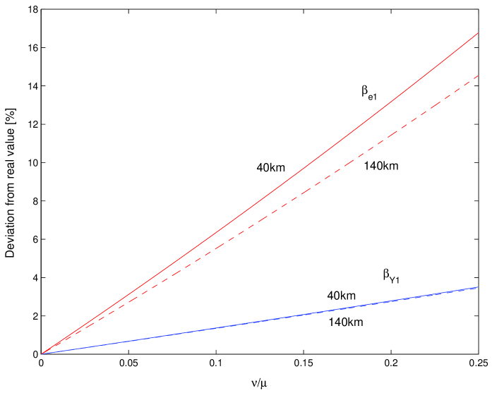
Figure 1: (Color Online) The solid lines show the relative deviations of $Y_{1}^{L,\nu_{1},\nu_{2}}$ and $e_{1}^{U,\nu_{1},\nu_{2}}$ from the asymptotic values (i.e., the case $\nu_{1},\nu_{2}\to 0$) as functions of $\nu/\mu$ (where $\nu=\nu_{1}$) with the fiber length 40km and the dashed lines show the case of 140km. The bounds $Y_{1}^{L,\nu_{1},\nu_{2}}$ and $e_{1}^{U,\nu_{1},\nu_{2}}$ are given by Eqs. (34) and (37), and the true values are given by Eqs. (7) and (9). We consider Vacuum+Weak protocol here ($\nu_{1}=\nu$ and $\nu_{2}=0$). The expected photon number is $\mu=0.48$ as calculated from Eq. (12). The parameters used are from GYS [5] as listed in Table 1.

Let $R^{L}$ denote for the lower bound of key generation rate, according to (1),

$$R^{L}=q\{-Q_{\mu}f(E_{\mu})H_{2}(E_{\mu})+Q_{1}^{L,\nu,0}[1-H_{2}(e_{1}^{U,\nu,0})]\},$$ (42)

where $q=\frac{1}{2}$ with standard BB84. The parameters can be calculated from Eqs. (10), (11), (35) and (37) and use $f(e)=1.22$, which is the upper bound of $f(e)$ in secure distance for this experiment [12]. Eq. (5) shows the relationship between $\eta$ and distance. The results are shown in Figure 2.

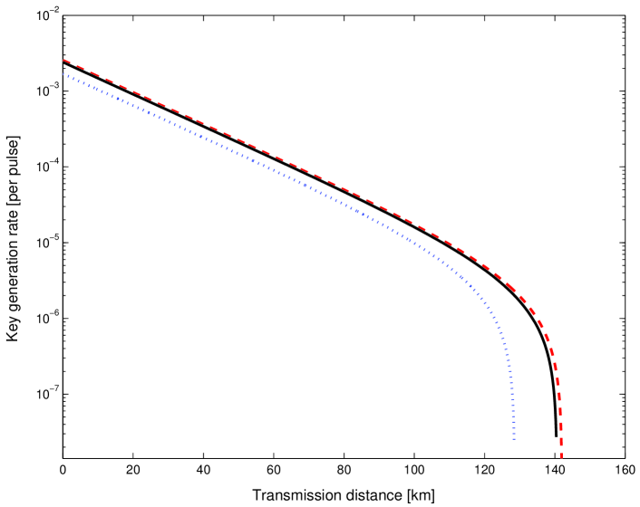
Figure 2: (Color Online) The dashed line shows the asymptotic decoy state method (with infinite number of decoy states) with a maximal secure distance of $142.05km$, using Eq. (1). The solid line shows our Vacuum+Weak decoy method, Eq. (42), with $\mu=0.48$, $\nu_{1}=0.05$ and $\nu_{2}=0$. It uses a strong version of GLLP and its maximal distance is $140.55km$. The dotted line shows the asymptotic case of Wang’s decoy method, Eq. (43) with $\mu=0.30$. It uses a weak version of GLLP and its maximal distance is about $128.55km$. This shows that our Vacuum+Weak decoy protocol performs very close to the asymptotic limit and performs better than even the asymptotic case of Wang’s decoy method. The data are from GYS [5] as listed in Table 1.

Now, from Figure 2, we can see that even with finite $\nu$ (say, $0.05$), Vacuum+Weak protocol performs very close to the asymptotic one.

We note that Wang [13] has also studied a decoy state protocol, first proposed by us [9], with only two decoy states for the special case where one of them is a vacuum. In [13] the second decoy state is used to estimate the multi photon fraction $\Delta$ and use the formula directly from GLLP [7] to calculate the key generation rate by Eq. (3).

In Figure 2, we compare the key generation rates of our two-decoy-state method and Wang’s method [13] and find that our method performs better. In what follows, we compare the differences between our method and that of Wang.

• We consider error correction inefficiency $f(e)$ for practical protocols. Wang did not consider this real-life issue. For a fair comparison, we add this factor to Eq. (3)

  $$R\geq qQ_{\mu}\{-f(E_{\mu})H_{2}(E_{\mu})+(1-\Delta)[1-H_{2}(\frac{E_{\mu}}{1-\Delta})]\}.$$ (43)

• Apparently, the value of $\mu$ was chosen in [13] in an ad hoc manner, whereas we performed optimization in Subsection 3.1 and found that for GYS, the optimal value of $\mu=0.48$ for our two-decoy-state method. Now, the best (asymptotic) estimate Wang’s method can make is that $\Delta=\mu$ when $\mu^{\prime}\rightarrow\mu$. For a fair comparison, we have performed an optimization of Wang’s asymptotic result Eq. (43) as well (similar to Subsection 3.1) and found that the value $\mu\approx 0.30$ optimizes the key generation rate in Wang’s method.

• In Eqs. (27) and (28), we show that our two-decoy-state method approaches a fundamental limit of the decoy state (the infinite decoy state protocol) while the asymptotic result in Wang [13] is strictly bounded away from the fundamental limit. Even with a finite $v_{1}$, our Vacuum+Weak protocol is better than Wang’s asymptotic case.

• Why do we get a stronger result than Wang’s [13]? Wang did not estimate $e_{1}$ and used $E_{\mu}/(1-\Delta)$ as the upper bound of $e_{1}$ (This corresponds to a weak version of GLLP [7]). We estimate $e_{1}$ more accurately following GLLP (a strong version of GLLP result).

4 Statistical Fluctuations

In this section, we would like to discuss the effect of finite data size in real life experiments on our estimation process for $Y_{1}$ and $e_{1}$. We will also discuss how statistical fluctuations might affect our choice of $\nu_{1}$ and $\nu_{2}$. We will provide a list of those fluctuations and discuss how we will deal with them. We remark that Wang [13] has previously considered the issue of fluctuations of $Y_{1}$.

All real-life experiments are done in a finite time. Ideally, we would like to consider a QKD experiment that can be performed within say a few hours or so. This means that our data size is finite. Here, we will see that this type of statistical fluctuations is a rather complex problem. We do not have a full solution to the problem. Nonetheless, we will provide some rough estimation based on standard error analysis which suggests that the statistical fluctuation problem of the two-decoy-state method for a QKD experiment appears to be under control, if we run an experiment over only a few hours.

4.1 What parameters are fluctuating?

Recall that from Eq. (1), there are four parameters that we need to take into account: the gain $Q_{\mu}$ and QBER $E_{\mu}$ of signal state and the gain $Q_{1}$ and QBER $e_{1}$ of single photon sate. The gain of signal state $Q_{\mu}$ is measured directly from experiment. We note that the fluctuations of the signal error rate $E_{\mu}$ is not important because $E_{\mu}$ is not used at all in the estimation of $Y_{1}$ and $e_{1}$. (See Eqs. (21) and (25) or Eqs. (35) and (37).) Therefore, the important issue is the statistical fluctuations of $Q_{1}$ and $e_{1}$ due to the finite data size of signal states and decoy states.

To show the complexity of the problem, we will now discuss the following five sources of fluctuations. The first thing to notice is that, in practice, the intensity of the lasers used by Alice will be fluctuating. In other words, even the parameters $\mu$, $\nu_{1}$ and $\nu_{2}$ suffer from small statistical fluctuations. Without hard experimental data, it is difficult to pinpoint the extent of their fluctuations. To simplify our analysis, we will ignore their fluctuations in this paper.

The second thing to notice is that so far in our analysis we have assumed that the proportion of photon number eigenstates in each type of state is fixed. For instance, if $N$ signal states of intensity $\mu$ are emitted, we assume that exactly $N\mu e^{-\mu}$ out of the $N$ signal states are single photons. In real-life, the number $\mu e^{-\mu}$ is only a probability, the actual number of single photon signals will fluctuate statistically. The fluctuation here is dictated by the law of large number though. So, this problem should be solvable. For simplicity, we will neglect this source of fluctuations in this paper. [It was subsequently pointed out to us by Gottesman and Preskill that the above two sources of fluctuations can be combined into the fluctuations in the photon number frequency distribution of the underlying signal and decoy states. These fluctuations will generally average out to zero in the limit of a large number of signals, provided that there is no systematic error in the experimental set-up.]

The third thing to notice is, as noted by Wang [13], the yield $Y_{i}$ may fluctuate in the sense that $Y_{i}$ for the signal state might be slightly different from $Y^{\prime}_{i}$ of the decoy state. We remark that if one uses the vacuum state as one of the decoy states, then by observing the yield of the vacuum decoy state, conceptually, one has a very good handle on the yield of the vacuum component of the signal state (in terms of hypergeometric functions). Note, however, that the background rate is generally rather low (typically $10^{-5}$). So, to obtain a reasonable estimation on the background rate, a rather large number (say $10^{7}$) of vacuum decoy states will be needed. [As noted in [9], even a $20\%$ fluctuations in the background will have small effect on the key generation rates and distances.] Note that, with the exception of the case $n=0$ (the vacuum case), neither $Y_{i}$ and $Y_{i}^{\prime}$ are directly observable in an experiment. In a real experiment, one can measure only some averaged properties. For instance, the yield $Q_{\mu}$ of the signal state, which can be experimentally measured, has its origin as the weighted averaged yields of the various photon number eigenstates $Y_{i}$’s whereas that for the decoy state is given by the weighted averaged of $Y^{\prime}_{i}$’s. How to relate the observed averaged properties, e.g., $Q_{\mu}$, to the underlying values of $Y_{i}$’s is challenging question. In summary, owing to the fluctuations of $Y_{i}$ for $n>0$, it is not clear to us how to derive a closed form solution to the problem.

Fourth, we note that the error rates, $e_{i}$’s, for the signal can also be different from the error rates $e_{i}$’s for the decoy state, due to underlying statistical fluctuations. Actually, the fluctuation of $e_{1}$ appears to the dominant source of errors in the estimation process. (See, for example, Table 2.) This is because the parameter $e_{1}$ is rather small (say a few percent) and it appears in combination with another small parameter $Y_{1}$ in Eq. (11) for QBER.

Fifth, we noted that for security in the GLLP [7] formula (Eq. (1)), we need to correct phase errors, rather than bit-flip errors. From Shor-Preskill’s proof [3], we know that the bit-flip error rate and the phase error rate are supposed to be the same only in the asymptotic limit. Therefore, for a finite data set, one has to consider statistical fluctuations. This problem is well studied [3]. Since the number of signal states is generally very big, we will ignore this fluctuation from now on.

Qualitatively, the yields of the signal and decoy states tend to decrease exponentially with distance. Therefore, statistical fluctuations tend to become more and more important as the distance of QKD increases. In general, as the distance of QKD increases, larger and large data sizes will be needed for the reliable estimation of $Y_{1}$ and $e_{1}$ (and hence $R$), thus requiring a longer QKD experiment.

In this paper, we will neglect the fluctuations due to the first two and the fifth sources listed above. Even though we cannot find any closed form solution for the third and fourth sources of fluctuations, it should be possible to tackle the problem by simulations. Here, we are contented with a more elementary analysis. We will simply apply standard error analysis to perform a rough estimation on the effects of fluctuations due to the third and fourth sources. We remark that the origin of the problem is strictly classical statistical fluctuations. There is nothing quantum in this statistical analysis. While standard error analysis (using essentially normal distributions) may not give a completely correct answer, we expect that it is correct at least in the order of magnitude.

Our estimation, which will be presented below, shows that, for long-distance ($>100km$) QKD with our two-decoy-state protocol, the statistical fluctuations effect (from the third and fourth sources only) appears to be manageable. This is so provided that a QKD experiment is run for a reasonable period of time of only a few hours. Our analysis supports the viewpoint that our two-decoy-state protocol is practical for real-life implementations.

We remark on passing that the actual classical memory space requirement for Alice and Bob is rather modest ($<1GBytes$) because at long distance, only a small fraction of the signals will give rise to detection events.

We emphasize that we have not fully solved the statistical fluctuation problem for decoy state QKD. This problem turns out to be quite complex. We remark that this statistical fluctuation problem will affect all earlier results including [8, 9, 13]. In future investigations, it will be interesting to study the issues of classical statistical fluctuations in more detail.

4.2 Standard Error Analysis

In what follows, we present a general procedure for studying the statistical fluctuations (due to the third and fourth sources noted above) by using standard error analysis.

Denote the number of pulses (sent by Alice) for signal as $N_{S}$, and for two decoy states as $N_{1}$ and $N_{2}$. Then, the total number of pulses sent by Alice is given by

$$N =N_{S}+N_{1}+N_{2}.$$ (44)

Then the parameter $q$ in Eq. (1) is given by

$$q =\frac{N_{S}}{2N}.$$ (45)

Here we assume Alice and Bob perform standard BB84. So, there is a factor of $\frac{1}{2}$.

In practice, since $N$ is finite, the statistical fluctuations of $Q_{1}$ and $e_{1}$ cannot be neglected. All these additional deviations will be related to data sizes $N_{S}$, $N_{1}$ and $N_{2}$ and can, in principle, be obtained from statistic analysis. A natural question to ask is the following. Given total data size $N=const$, how to distribute it to $N_{S}$, $N_{1}$ and $N_{2}$ to maximize the key generation rate $R$? This question also relates to another one: how to choose optimal weak decoy $\nu_{1}$ and $\nu_{2}$ to minimize the effects of statistical fluctuations?

In principle, our optimization procedure should go as follows. First, (this is the hard part) one needs to derive a lower bound of $Q_{1}$ and an upper bound of $e_{1}$ (as functions of data size $N_{S}$, $N_{1}$, $N_{2}$, $\nu_{1}$ and $\nu_{2}$), taking into full account of statistical fluctuations. Second, one substitutes those bounds to Eq. (1) to calculate the lower bound of the key generation rate, denoted by $R^{L}$. Thus, $R^{L}$ is a function of $N_{S}$, $N_{1}$, $N_{2}$, $\nu_{1}$ and $\nu_{2}$, and will be maximized when the optimal distribution satisfies

$$\frac{\partial R^{L}}{\partial N_{S}}=\frac{\partial R^{L}}{\partial N_{1}}=\frac{\partial R^{L}}{\partial N_{2}}=0,$$ (46)

given $N=N_{S}+N_{1}+N_{2}=const$.

4.3 Choice of $\nu_{1}$ and $\nu_{2}$

Now, from the theoretical deviations of $Y_{1}$ and $e_{1}$, Eqs. (29) and (30), reducing $\nu$ may decrease the theoretical deviations. We need to take statistical fluctuations into account. Given a fixed $N_{1}+N_{2}$, reducing $\nu_{1}$ and $\nu_{2}$ will decrease the number of detection events of decoy states, which in turns causes a larger statistical fluctuation. Thus, there exists an optimal choice of $\nu_{1}$ and $\nu_{2}$ which maximizes the lower bound of the key generation rate $R^{L}$,

$$\frac{\partial R^{L}}{\partial\nu_{1}}=\frac{\partial R^{L}}{\partial\nu_{2}}=0,\\$$

which can be simplified to

$$\frac{\partial}{\partial\nu_{1}}\{\hat{Y}_{1}^{L,\nu_{1},\nu_{2}}[1-H_{2}(\hat{e}_{1}^{U,\nu_{1},\nu_{2}})]\} =0$$ (47)

$$\frac{\partial}{\partial\nu_{2}}\{\hat{Y}_{1}^{L,\nu_{1},\nu_{2}}[1-H_{2}(\hat{e}_{1}^{U,\nu_{1},\nu_{2}})]\} =0,$$

where $\hat{Y}_{1}^{L,\nu_{1},\nu_{2}}$ and $\hat{e}_{1}^{U,\nu_{1},\nu_{2}}$ are lower bound to $Y_{1}$ and upper bound to $e_{1}$ when statistical fluctuations are considered.

Given total data size in Eq. (44), in principle, one can solve Eqs. (46) and (47) to get $N_{S}$, $N_{1}$, $N_{2}$ $\nu_{1}$ and $\nu_{2}$.

4.4 Simulation:

In real life, solving Eqs. (46) and (47) is a complicated problem. In what follows, we will be contented with a rough estimation procedure using standard error analysis commonly used by experimentalists.

Some assumptions: In the following, we will discuss Vacuum+Weak decoy method only.

1. The signal state is used much more often than the two decoy states. Given the large number of signal states, it is reasonable to ignore the statistical fluctuations in signal states.

2. We assume that the decoy state used in the actual experiment is conceptually only a part of an infinite population of decoy states. There are underlying values for $Q_{\nu}$ and $E_{\nu}$ as defined by the population of decoy states. In each realization, the decoy state allows us to obtain some estimates for these underlying $Q_{\nu}$ and $E_{\nu}$ . Alice and Bob can use the fluctuations of $Q_{\nu}$, $E_{\nu}$ to calculate the fluctuation of the estimates of $Y_{1}$ and $e_{1}$.

3. We neglect the change of $f(E_{\mu})$ due to small change in $E_{\mu}$.

4. When the number of events (e.g. the total detection event of the vacuum decoy state) is large (say $>50$), we assume that the statistical characteristic of a parameter can be described by a normal distribution.

We will use the experiment parameters in Table 1 and show numerical solutions of Eqs. (44), (46) and (47). We pick the total data size to be $N=6\times 10^{9}$. Now, the GYS experiment [5] has a repetition rate of $2MHz$ and an up time of less than $50\%$ [19]. Therefore, it should take only a few hours to perform our proposed experiment. The optimal $\mu=0.48$ can be calculated by Eq. (12) and we use $f(e)=1.22$.

In the fiber length of $103.62km$ ($\eta=3\times 10^{-4}$), the optimal pulses distribution of data, $\nu$ and the deviations from perfect decoy method are listed in Table 2.

$l$	$\mu$	$u_{\alpha}$	$N$	$N_{S}$	$N_{1}$	$N_{2}$
$103.62km$	$0.479$	$10$	$6\times 10^{9}$	$3.98\times 10^{9}$	$1.76\times 10^{9}$	$2.52\times 10^{8}$
$\eta$	$\nu$	$\tilde{B}[bits]$	$\beta_{Y0}$	$\beta_{Y1}$	$\beta_{e1}$	$\beta_{R}$
$3\times 10^{-4}$	$0.127$	$2.17\times 10^{4}$	$48.31\%$	$7.09\%$	$97.61\%$	$74.11\%$

Table 2: The pulse number distribution and $\nu$ are calculated from Eqs. (46) and (47). $\tilde{B}$ is the lower bound of final key bits. All results are obtained by numerical analysis using MatLab. The variable $\tilde{\beta}_{Y1}$ denotes the relative error in our estimation process of $Y_{1}$ from its true value by using the data from a finite experiment. This relative error originates from statistical fluctuations. This definition contrasts with the definition of $\beta_{Y1}$ in Eq. (29) which refers to the relative difference between the values of $Y_{1}$ for the case i) where $\nu_{1}$ and $\nu_{2}$ are finite and the case ii) where $\nu_{1}$ and $\nu_{2}$ approach zero. Similarly, other $\beta$’s denote the relative errors in our estimates for the corresponding variables in the subscript of $\beta$. All the statistical fluctuation is of the confidence interval of ten standard deviations (i.e., $1-1.5\times 10^{-23}$). The data come from GYS [5], listed in Table 1.

For each fiber length we can solve Eqs. (46) and (47) to get $N_{S}$, $N_{E}$, $N_{1}$, $N_{2}$ and $\nu$.

Figure 3 shows how the optimal $\nu$ changes with fiber length. We can see that the optimal $\nu$ is small ($\sim 0.1$) through the whole distance. In fact, it starts at a value $\nu\approx 0.04$ at zero distance and increases almost linearly with the distance.

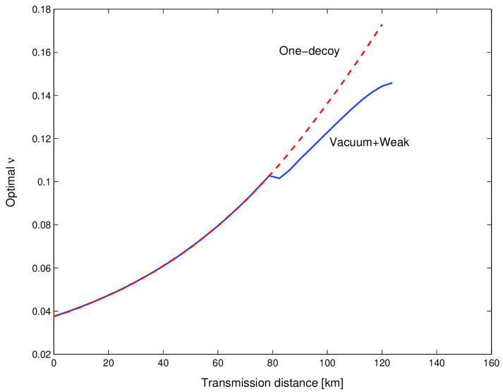
Figure 3: (Color Online) The solid line shows the simulation result of the Vacuum+Weak protocol (Eqs. (34) and (37)) with statistical fluctuations. The dashed line shows the result for one-decoy-state method (Eqs. (41)). Here, we pick the data size (total number of pulses emitted by Alice) to be $N=6\times 10^{9}$. We find the optimal $\nu$’s for each fiber length by numerically solving Eqs. (44), (46) and (47). The confidence interval for statistical fluctuation is ten standard deviations (i.e., $1-1.5\times 10^{-23}$). The data are from GYS [5] as listed in Table 1. The expected photon number of signal state is calculated by Eq. (12), getting $\mu=0.48$. The second decoy state (vacuum decoy) becomes useful at 82km.

Figure 4 shows Vacuum+Weak with statistical fluctuations as compared to the asymptotic case of infinite decoy state and without statistical fluctuations. We can see that even taking into account the statistical fluctuations, the Vacuum+Weak protocol is not far from the asymptotic result. In particular, in the short distance region, our two-decoy-state method with statistical fluctuations approaches the performance of the asymptotic limit of infinite decoy states and no statistical fluctuations. This is so because the channel is not that lossy and statistical fluctuations are easily under control. This fact highlights the feasibility of our proposal.

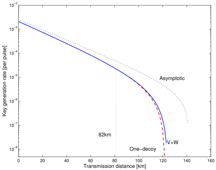
Figure 4: (Color Online) The dotted line shows the performance of perfect decoy state method (with infinite number of decoy states and no statistical fluctuations). The maximal distance is about 142km. The solid line shows the simulation result of the Vacuum+Weak protocol (Eqs. (34) and (37)) with statistical fluctuations. Its maximal distance is about 125km. The dashed line shows the result for one-decoy-state method (Eqs. (41)) with maximal distance 122km. We pick a data size (i.e., total number of pulses emitted by Alice) to be $N=6\times 10^{9}$. Note that even with statistical fluctuations and a rather modest data size, our Vacuum+Weak decoy protocol performs rather close to asymptotic limit, particularly at short distances. The second decoy state (vacuum decoy) becomes useful at 82km. The data are from GYS [5] as listed in Table 1. The expected photon number of signal state is calculated by Eq. (12), getting $\mu=0.48$.

Wang [13] picked the total data size $N=8.4\times 10^{10}$. For long distance QKD, this will take more than one day of experiment with the current GYS set-up [5]. In order to perform a fair comparison with Wang[13]’s result, we will now the data size $N=8.4\times 10^{10}$. Figure 5 shows $R^{L}$ vs. fiber length $l$ with $N=8.4\times 10^{10}$ fixed and compares our Vacuum+Weak protocol with Wang’s result.

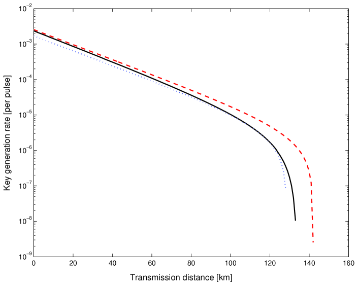
Figure 5: (Color Online) Here, we consider the data size (i.e., the number of pulses emitted by Alice) to be $N=8.4\times 10^{10}$, following Wang [13]. The dashed line shows the performance of perfect decoy state method. Its maximal distance is 142km. The solid line shows the simulation result of the Vacuum+Weak decoy state method with statistical fluctuations. Its maximal distance is 132km. The dotted line shows the asymptotic case (i.e., an idealized version) of Wang’s method. Its maximal distance is 128.55km. This figure shows clearly that with a data size $N=8.4\times 10^{10}$, our protocol, which considers statistical fluctuations, performs better even than the idealized version of Wang’s protocol, where statistical fluctuations are neglected. For our asymptotic case and two-decoy with statistical fluctuation $\mu=0.48$, and for Wang’s asymptotic case $\mu=0.3$, which are optimized.

Comments:

• Wang [13] chooses the value of $\mu$ in an ad hoc manner. Here we note that, for Wang’s asymptotic case, the optimal choice of $\mu$ is $\mu\in[0.25,0.3]$

• Even if we choose $\mu\in[0.25,0.3]$, the maximal secure distance of Wang’s asymptotic case is still less than our two-decoy-state method with statistical fluctuations. In other words, the performance of our two-decoy-state method with statistical fluctuations is still better than the the asymptotic value (i.e., without considering statistical fluctuations) given by Wang’s method.

• Note that GYS [5] has a very low background rate ($Y_{0}=1.7\times 10^{-6}$) and high $e_{detector}$. The typical values of these two key parameters are $Y_{0}=10^{-5}$ and $e_{detector}=1\%$. If the background rate is higher and $e_{detector}$ is lower, then our results will have more advantage over Wang’s. We illustrate this fact in Figure 6 by using the data from the KTH experiment [18].

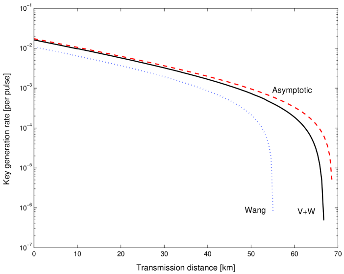
Figure 6: (Color Online) Here, we compare various protocols using the parameters in KTH [18], listed in Table 1 and [17]. The dashed line shows the performance of perfect decoy state method. It has a maximal secure distance of about 68.6km. The solid line shows the simulation result of the Vacuum+Weak decoy state method with statistical fluctuations. The maximal distance is about 67.2km). The dotted line shows the asymptotic case (i.e., neglecting statistical fluctuations) of Wang’s method whose maximal distance is about 55.5km. For our asymptotic case and two-decoy with statistical fluctuation $\mu=0.77$, and for Wang’s asymptotic case $\mu=0.43$, which are optimized.

5 Conclusion

We studied the two-decoy-state protocol where two weak decoy states of intensities $\nu_{1}$ and $\nu_{2}$ and a signal state with intensity $\mu$ are employed. We derived a general formula for the key generation rate $R$ of the protocol and showed that the asymptotically limiting case where $\nu_{1}$ and $\nu_{2}$ tend to zero gives an optimal key generation rate which is the same as having infinite number of decoy states. This result seems to suggest that there is no fundamental conceptual advantage in using more than two decoy states. Using the data from the GYS experiment [5], we studied the effect of finite $\nu_{1}$ and $\nu_{2}$ on the value of the key generation rate, $R$. In particular, we considerd a Vacuum+Weak protocol, proposed in [9] and analyzed in [13], where $\nu_{2}=0$ and showed that $R$ does not change much even when $\nu_{1}/\mu$ is as high as $25\%$. We also derived the optimal choice of expected photon number $\mu$ of the signal state, following our earlier work [9]. Finally, we considered the issue of statistical fluctuations due to a finite data size. We remark that statistical fluctuations have also been considered in the recent work of Wang [13]. Here, we listed five different sources of fluctuations. While the problem is highly complex, we provided an estimation based on standard error analysis. We believe that such an analysis, while not rigorous, will give at least the correct order of magnitude estimation to the problem. This is so because this is a classical estimation problem. There is nothing quantum about it. That is to say there are no subtle quantum attacks to consider. Our estimation showed that two-decoy-state QKD appears to be highly practical. Using data from a recent experiment [5], we showed that, even for long-distance (i..e, over 100km) QKD, only a few hours of data are sufficient for its implementation. The memory size requirement is also rather modest ($<1GBytes$). A caveat is that we have not considered the fluctuations of the laser intensities of Alice, i.e., the value of $\mu$, $\nu_{1}$ and $\nu_{2}$. This is because we do not have reliable experimental data to perform such an investigation. For short-distance QKD, the effects of statistical fluctuations are suppressed because the transmittance and useful data rate are much higher than long-distance QKD. Finally, we noted that statistical fluctuations will affect our choice of decoy states $\nu_{1}$ and $\nu_{2}$ and performed an optimization for the special case where $\nu_{2}=0$.

In summary, our investigation demonstrates that a simple two decoy state protocol with Vacuum+Weak decoy state is highly practical and can achieve unconditional security for long-distance (over 100km) QKD, even with only a few hours of experimental data.

As a final note, we have also studied a simple one-decoy-state protocol. Recently, we have experimentally implemented our one-decoy-state protocol over 15km of Telecom fibers [15], thus demonstrating the feasibility of our proposal.

Appendix A Appendix

In this appendix, we will prove that the Vacuum+Weak decoy protocol is optimal among the two-weak-decoy protocol. We do so by proving that, for a fixed $\nu_{1}$ (which is larger than $\nu_{2}$),

• the lower bound $Y_{1}^{L,\nu_{1},\nu_{2}}$ can be no greater than $Y_{1}^{L,\nu_{1},0}$, see Eq.(55)

• the upper bound $e_{1}^{U,\nu 1,\nu 2}$ can be no less than $e_{1}^{U,\nu 1,0}$, see Eq. (57)

We will consider those bounds as given in Eqs. (21) and (25). In what follows, we assume the conditions given by Eq. (15),

$$0\leq\nu_{2}<\nu_{1}$$ (48)

$$\nu_{1}+\nu_{2}<\mu.$$

Theorem Given $\mu$, $\nu_{1}$, $\eta$, $Y_{0}$ and $e_{detector}$, the lower bound of $Y_{1}$ given in Eq. (21),

$$Y_{1}^{L,\nu_{1},\nu_{2}} =\frac{\mu}{\mu\nu_{1}-\mu\nu_{2}-\nu_{1}^{2}+\nu_{2}^{2}}(Q_{\nu_{1}}e^{\nu_{1}}-Q_{\nu_{2}}e^{\nu_{2}}-\frac{\nu_{1}^{2}-\nu_{2}^{2}}{\mu^{2}}Q_{\mu}e^{\mu})$$

is a decreasing function of $\nu_{2}$, and the upper bound of $e_{1}$ given in Eq. (25),

$$e_{1}^{U,\nu_{1},\nu_{2}} =\frac{E_{\nu_{1}}Q_{\nu_{1}}e^{\nu_{1}}-E_{\nu_{2}}Q_{\nu_{2}}e^{\nu_{2}}}{(\nu_{1}-\nu_{2})Y_{1}^{L,\nu_{1},\nu_{2}}}$$

is an increasing function of $\nu_{2}$, under conditions Eq. (48). Here $Q_{\mu}$, $Q_{\nu_{1}}$, $Q_{\nu_{2}}$, $E_{\mu}$, $E_{\nu_{1}}$ and $E_{\nu_{2}}$ are given by Eqs. (10) and (11).

Proof of the theorem First we will prove $Y_{1}^{L,\nu_{1},\nu_{2}}$ is a decreasing function of $\nu_{2}$ and then prove $e_{1}^{U,\nu_{1},\nu_{2}}$ is an increasing function of $\nu_{2}$.

Define functions $G(\mu)$ and $J(\mu)$ as

$$G(\mu) =Q_{\mu}e^{\mu}$$

$$=(Y_{0}+1-e^{-\eta\mu})e^{\mu}$$

$$J(\mu) =E_{\mu}Q_{\mu}e^{\mu}$$

$$=[e_{0}Y_{0}+e_{detector}(1-e^{-\eta\mu})]e^{\mu}.$$

Take the first derivative of $G(\mu)$ and $J(\mu)$,

$$G^{\prime}(\mu) =Q_{\mu}e^{\mu}+\eta e^{(1-\eta)\mu}$$

$$J^{\prime}(\mu) =E_{\mu}Q_{\mu}e^{\mu}+\eta e_{detector}e^{(1-\eta)\mu},$$

which are both increasing functions and $G^{\prime}(\mu)\geq 0$, $J^{\prime}(\mu)\geq 0$. By mathematical induction, it is not difficult to prove the following claim.

Claim 1: For any order derivative of $G(\mu)$ and $J(\mu)$: $G^{(n)}(\mu)\geq 0$ and $J^{(n)}(\mu)\geq 0$ are increasing functions.

Some Useful Inequalities: With Claim 1 and the Taylor Series of $G(\mu)$, we have

$$G(\mu) =\sum_{i=0}^{i=\infty}G^{(i)}(\mu)\frac{\mu^{i}}{i!}$$ (49)

$$\geq\mu G^{\prime}(\mu)$$

According to Mean Value Theorem,

$$\frac{G(\nu_{1})-G(\nu_{2})}{\nu_{1}-\nu_{2}}=G^{\prime}(\nu_{3})$$ (50)

$$\frac{J(\nu_{1})-J(\nu_{2})}{\nu_{1}-\nu_{2}}=J^{\prime}(\nu_{4})$$

where $\nu_{3},\nu_{4}\in[\nu_{2},\nu_{1}]$. Because $G^{\prime}(\mu)$ and $J^{\prime}(\mu)$ are increasing functions, we can bound Eq. (50),

$$G^{\prime}(\nu_{2})\leq\frac{G(\nu_{1})-G(\nu_{2})}{\nu_{1}-\nu_{2}}\leq G^{\prime}(\nu_{1})$$ (51)

$$J^{\prime}(\nu_{2})\leq\frac{J(\nu_{1})-J(\nu_{2})}{\nu_{1}-\nu_{2}}\leq J^{\prime}(\nu_{1}).$$ (52)

Similarly,

$$G^{\prime\prime}(\nu_{2})\leq\frac{G^{\prime}(\nu_{1})-G^{\prime}(\nu_{2})}{\nu_{1}-\nu_{2}}\leq G^{\prime\prime}(\nu_{1}).$$ (53)

Define a function

$$F(\nu_{2}) =\frac{1}{\mu-\nu_{1}-\nu_{2}}[Q_{\mu}e^{\mu}-\frac{\mu}{\nu_{1}-\nu_{2}}(Q_{\nu_{1}}e^{\nu_{1}}-Q_{\nu_{2}}e^{\nu_{2}})]$$

$$=\frac{1}{\mu-\nu_{1}-\nu_{2}}[G(\mu)-\frac{\mu}{\nu_{1}-\nu_{2}}(G({\nu_{1}})-G({\nu_{2}}))]$$

Claim 2: The function $F(\nu_{2})$ is an increasing function of $\nu_{2}$, under the conditions given in Eq. (48).

Proof of Claim 2: To determine if the function is increasing or decreasing we will need the derivative.

$$F^{\prime}(\nu_{2})= \frac{1}{(\mu-\nu_{1}-\nu_{2})^{2}}[G(\mu)-\frac{\mu}{\nu_{1}-\nu_{2}}(G({\nu_{1}})-G({\nu_{2}}))]$$ (54)

$$-\frac{1}{\mu-\nu_{1}-\nu_{2}}\frac{\mu}{(\nu_{1}-\nu_{2})^{2}}[G({\nu_{1}})-G({\nu_{2}})]$$

$$+\frac{1}{\mu-\nu_{1}-\nu_{2}}\frac{\mu}{\nu_{1}-\nu_{2}}G^{\prime}({\nu_{2}})$$

$$\geq \frac{1}{(\mu-\nu_{1}-\nu_{2})^{2}}[G(\mu)-\mu G^{\prime}({\nu_{1}})]$$

$$-\frac{1}{\mu-\nu_{1}-\nu_{2}}\frac{\mu}{\nu_{1}-\nu_{2}}G^{\prime}({\nu_{1}})+\frac{1}{\mu-\nu_{1}-\nu_{2}}\frac{\mu}{\nu_{1}-\nu_{2}}G^{\prime}({\nu_{2}})$$

$$\geq \frac{1}{(\mu-\nu_{1}-\nu_{2})^{2}}[\mu G^{\prime}(\mu)-\mu G^{\prime}({\nu_{1}+\nu_{2}})]-\frac{\mu}{\mu-\nu_{1}-\nu_{2}}G^{\prime\prime}({\nu_{1}})$$

$$\geq \frac{\mu}{\mu-\nu_{1}-\nu_{2}}[G^{\prime\prime}({\nu_{1}+\nu_{2}})-G^{\prime\prime}({\nu_{1}})]$$

$$\geq 0$$

Here, to prove the first inequality, we have made use of Eq. (51); to prove the second inequality, we have made use of Eq. (49), (53) and Claim 1; to prove the third inequality, we have made use of Eq. (53); to prove the last inequality, we have made use of Claim 1.

Proof that $Y_{1}^{L,\nu_{1},\nu_{2}}$ is a decreasing function. Re-write the lower bound of $Y_{1}$, in Eq. (21),

$$Y_{1}^{L,\nu_{1},\nu_{2}} =\frac{\mu}{\mu\nu_{1}-\mu\nu_{2}-\nu_{1}^{2}+\nu_{2}^{2}}(Q_{\nu_{1}}e^{\nu_{1}}-Q_{\nu_{2}}e^{\nu_{2}}-\frac{\nu_{1}^{2}-\nu_{2}^{2}}{\mu^{2}}Q_{\mu}e^{\mu})$$ (55)

$$=\frac{\mu}{\mu\nu_{1}-\mu\nu_{2}-\nu_{1}^{2}+\nu_{2}^{2}}(Q_{\nu_{1}}e^{\nu_{1}}-Q_{\nu_{2}}e^{\nu_{2}})-\frac{\mu}{\mu\nu_{1}-\mu\nu_{2}-\nu_{1}^{2}+\nu_{2}^{2}}\frac{\nu_{1}^{2}-\nu_{2}^{2}}{\mu^{2}}Q_{\mu}e^{\mu}$$

$$=\frac{\mu}{\mu-\nu_{1}-\nu_{2}}\frac{Q_{\nu_{1}}e^{\nu_{1}}-Q_{\nu_{2}}e^{\nu_{2}}}{\nu_{1}-\nu_{2}}-\frac{\nu_{1}+\nu_{2}}{\mu-\nu_{1}-\nu_{2}}\frac{Q_{\mu}e^{\mu}}{\mu}$$

$$=\frac{\mu}{\mu-\nu_{1}-\nu_{2}}\frac{Q_{\nu_{1}}e^{\nu_{1}}-Q_{\nu_{2}}e^{\nu_{2}}}{\nu_{1}-\nu_{2}}-(\frac{1}{\mu-\nu_{1}-\nu_{2}}-\frac{1}{\mu})Q_{\mu}e^{\mu}$$

$$=\frac{1}{\mu}Q_{\mu}e^{\mu}-\frac{1}{\mu-\nu_{1}-\nu_{2}}[Q_{\mu}e^{\mu}-\frac{\mu}{\nu_{1}-\nu_{2}}(Q_{\nu_{1}}e^{\nu_{1}}-Q_{\nu_{2}}e^{\nu_{2}})]$$

$$=\frac{1}{\mu}Q_{\mu}e^{\mu}-F(\nu_{2}).$$

With Claim 2, we show that $Y_{1}^{L,\nu_{1},\nu_{2}}$ is a decreasing function of $\nu_{2}$.

Define a function

$$K(\nu_{2}) =\frac{E_{\nu_{1}}Q_{\nu_{1}}e^{\nu_{1}}-E_{\nu_{2}}Q_{\nu_{2}}e^{\nu_{2}}}{\nu_{1}-\nu_{2}}$$

$$=\frac{J({\nu_{1}})-J({\nu_{2}})}{\nu_{1}-\nu_{2}}$$

Claim 3: function $K(\nu_{2})$ is an increasing function with $\nu_{2}$.

Proof: to determine if the function is increasing or decreasing we will need the derivative.

$$K^{\prime}(\nu_{2}) =\frac{J({\nu_{1}})-J({\nu_{2}})}{(\nu_{1}-\nu_{2})^{2}}-\frac{J^{\prime}({\nu_{2}})}{\nu_{1}-\nu_{2}}$$ (56)

$$\geq\frac{J^{\prime}({\nu_{2}})}{\nu_{1}-\nu_{2}}-\frac{J^{\prime}({\nu_{2}})}{\nu_{1}-\nu_{2}}$$

$$=0,$$

where the first inequality is due to Eq. (52).

Proof that $e_{1}^{U,\nu_{1},\nu_{2}}$ is an increasing function. Reform the lower bound of $e_{1}$, in Eq. (25),

$$e_{1}^{U,\nu_{1},\nu_{2}} =\frac{E_{\nu_{1}}Q_{\nu_{1}}e^{\nu_{1}}-E_{\nu_{2}}Q_{\nu_{2}}e^{\nu_{2}}}{(\nu_{1}-\nu_{2})Y_{1}^{L,\nu_{1},\nu_{2}}}$$ (57)

$$=\frac{K(\nu_{2})}{Y_{1}^{L,\nu_{1},\nu_{2}}}$$

With Claim 3 and decreasing function of $Y_{1}^{L,\nu_{1},\nu_{2}}$, we show that $e_{1}^{U,\nu_{1},\nu_{2}}$ is an increasing function of $\nu_{2}$.

In summary, we have proved the theorem.

References

- [1] Bennett, C. H. & Brassard, G., Proceedings of IEEE International Conference on Computers, Systems, and Signal Processing, IEEE, 1984, pp. 175-179.
- [2] Mayers, D. J. of ACM 48, 351 (2001). A preliminary version in Mayers, D. Advances in Cryptology–Proc. Crypto ’96, vol. 1109 of Lecture Notes in Computer Science, Koblitz, N. Ed. (Springer-Verlag, New York, 1996), pp. 343-357; Lo, H.-K. & Chau, H. F., Science, 283, 2050 (1999); Biham, E., Boyer, M., Boykin, P. O., Mor, T. & Roychowdhury, V., Proceedings of the Thirty-Second Annual ACM Symposium on Theory of Computing (STOC’00) (ACM Press, New York, 2000), pp. 715-724; Ben-Or, M. Presentation at MSRI, available on-line at http://www.msri.org/publications/ln/msri/2002/qip/ben-or/1/
- [3] P. W. Shor and J. Preskill, “Simple proof of security of the BB84 quantum key distribution protocol”, Phys. Rev. Lett., vol. 85, p. 441, 2000. Also, [*Online] Available: http://xxx.lanl.gov/abs/quant-ph/0003004.
- [4] A. K. Ekert, and B. Huttner, J. of Modern Optics 41, 2455 (1994); D. Deutsch et al., Phys. Rev. Lett. 77, 2818 (1996); Erratum: Phys. Rev. Lett. 80, 2022 (1998).
- [5] C. Gobby, Z. L. Yuan, and A. J. Shields, “Quantum key distribution over 122 km of standard telecom fiber”, Applied Physics Letters, Volume 84, Issue 19, pp. 3762-3764, (2004).
- [6] Kimura, T. et al., On-line available at http://arxiv.org/abs/quant-ph/0403104
- [7] D. Gottesman, H.-K. Lo, Norbert Lutkenhaus, and John Preskill, “Security of quantum key distribution with imperfect devices”, Quantum Information and Computation. Vol. 4, No.5 (2004) 325-360, http://arxiv.org/abs/quant-ph/0212066
- [8] W.-Y. Hwang, “Quantum Key Distribution with High Loss: Toward Global Secure Communication”, Phys. Rev. Lett. 91, 057901 (2003)
- [9] H.-K. Lo, X. Ma and K. Chen “Decoy State Quantum Key Distribution”, http://arxiv.org/abs/quant-ph/0411004 (accepted for publication in PRL). Preliminary results were presented in Proceedings of IEEE ISIT 2004, Page 137, IEEE Press, July 2004, and the Fields Institute Conference on Quantum Information and Quantum Control, http://www.fields.utoronto.ca/programs/scientific/04-05/quantumIC/abstracts/lo.ppt July 2004. See also X. Ma, “Security of Quantum Key Distribution with Realistic Devices,” Master Report submitted to the University of Toronto, Sept. 2004, available as http://arxiv.org/abs/quant-ph/0503057.
- [10] H.-K. Lo, H. F. Chau, and M. Ardehali, “Efficient Quantum Key Distribution Scheme And Proof of Its Unconditional Security”, J. of Cryptology, ISSN: 0933-2790 (Paper) 1432-1378 (Online) published online 3 March 2004, (10.1007/s00145-004-0142-y). (Springer-Verlag New York, LLC); available at http://arxiv.org/abs/quant-ph/0011056.
- [11] Here, the gain of a particular type of signals is defined to be the fraction of detection events by Bob that is due to that particular type of signals.
- [12] G. Brassard and L. Salvail, in Advances in Cryptology EUROCRYPT ’93, Vol. 765 of Lecture Notes in Computer Science, edited by T. Helleseth (Springer, Berlin, 1994), pp. 410-423.
- [13] Xiang-Bin Wang, “Beating the PNS attack in practical quantum cryptography”, http://arXiv:quant-ph/0410075, v5 24 Jan 2005 and “A decoy-state protocol for quantum cryptography with 4 intensities of coherent states” http://arxiv.org/abs/quant-ph/0411047 .
- [14] J. W. Harrington, J. M. Ettinger, R. J. Hughes, and J. E. Nordholt, “Enhancing practical security of quantum key distribution with a few decoy states”, available at http://arxiv.org/abs/quant-ph/0503002
- [15] Y. Zhao, B. Qi, X. Ma, H.-K. Lo and L. Qian, “Experimental Decoy State Quantum Key Distribution Over 15km”, http://arxiv.org/abs/quant-ph/0503192
- [16] M. Koashi, e-Print archive (available at http://arxiv.org/abs/quant-ph/0403131 ]
- [17] Norbert Lütkenhaus, “Security against individual attacks for realistic quantum key distribution”, Phys. Rev. A, Vol. 61, 052304 (2000); also available on-line as http://arxiv.org/abs/quant-ph/9910093
- [18] M. Bourennane, F. Gibson, A. Karlsson, A. Hening, P.Jonsson, T. Tsegaye, D. Ljunggren, and E. Sundberg, Opt. Express 4, 383 (1999).
- [19] Zhiliang Yuan, private communications regarding his GYS experiment [5].