Control of Local Relaxation Behavior in Closed Bipartite Quantum Systems

Abstract

We investigate the decoherence of a spin $1/2$ subsystem weakly coupled to an environment of many spins $1/2$ with and without mutual coupling. The total system is closed, its state is pure and evolves under Schrödinger dynamics. Nevertheless, the considered spin typically reaches a quasi-stationary equilibrium state.

Here we show that this state depends strongly on the coupling to the environment on the one hand and on the coupling within the environmental spins on the other. In particular we focus on spin star and spin ring-star geometries to investigate the effect of intra-environmental coupling on the central spin. By changing the spectrum of the environment its effect as a bath on the central spin is changed also and may even be adjustable to some degree. We find that the relaxation behavior is related to the distribution of the energy eigenstates of the total system.

For each of these relaxation modes there is a dual mode for which the resulting subsystem approaches an inverted state occupation probability (negative temperature).

I Introduction

In a composite but closed quantum system in which a smaller “central system” is weakly coupled to a larger “environment”, most of the (pure) states of the total system for a given energy (and possibly some additional constraints) exhibit properties of thermal equilibrium states with respect to the smaller part Gemmer et al. (2004); Gemmer and Mahler (2003), i.e. there exists a so-called dominant region in Hilbert space in which the entropy of the central system is close to its maximum value under the given constraints. For a completely “unstructured” coupling to the environment, the state of the central system, starting away from equilibrium, shows decoherence and thermalization and, ultimately, a quasi-stationary equilibrium situation is reached which is determined only by the spectrum of the environment Borowski et al. (2003).

In this paper we investigate to what extent structured systems will also exhibit this thermalization behavior. We focus, in particular, on a single central spin $1/2$ particle coupled to a relatively small environment of spin $1/2$ particles. Recently, the properties of spin systems of different structure (rings, stars and others) have been subject of extensive interest. A lot of work has been done on the question of entanglement Briegel and Raussendorf (2001); O’Connor and Wootters (2001); Wang (2002); Hutton and Bose (2004a, b); Vidal et al. (2003), their relaxation behavior has been addressed Breuer et al. (2004); Lages et al. (2004) and various techniques were suggested to make any spin interact with any other spin Imamoḡlu et al. (1999); Makhlin et al. (1999).

Here we show that by choosing different types of coupling between the central system and the environment on the one hand and within the environment on the other the equilibrium state finally reached can be controlled. There is, in particular, a qualitative difference between the relaxation dynamics and the equilibrium of the central spin for interacting and noninteracting environments. We relate this equilibrium to the spectral structure of the total system.

II Spectral Temperature

Consider a weakly coupled bipartite quantum system consisting of a small system S and a large “container” or environment C with the Hamiltonian

$$\hat{H}=\hat{H}^{\text{S}}+\hat{H}^{\text{C}}+\alpha\hat{H}^{\text{int}},\quad\mathinner{\langle\alpha\hat{H}^{\text{int}}\rangle}\ll\mathinner{\langle\hat{H}^{\text{S}}\rangle},\mathinner{\langle\hat{H}^{\text{C}}\rangle}.$$ (1)

The behavior of the system is completely described by a Hilbert space vector $\mathinner{\lvert\psi(t)\rangle}$ and its evolution under the Schrödinger equation. Under weak constraints, the state of S after relaxation is determined by Jaynes’ principle, taking energy as the only relevant observable Gemmer et al. (2004); Gemmer and Mahler (2003). The temperature of the respective canonical state can be predicted from the degeneracy structure of the environment alone.

Figure 1: Two-level system S in contact with environment C consisting of two highly degenerate levels $k$, $k^{\prime}$ with degeneracies $g_{k}$ and $g_{k^{\prime}}$, respectively. (a) Resonance, $\delta^{\text{S}}=\delta^{\text{C}}$, showing the state $\mathinner{\lvert 1\rangle}^{\text{S}}\otimes\mathinner{\lvert k,m\rangle}^{\text{C}}$ for which S evolves into a thermal state. (b) Slightly detuned energy splitting between S and C: Population relaxation in S is prohibited by energy conservation, C no longer acts as an effective heat bath.

Fig. 1(a) shows a two-level system in resonant contact with an environment consisting of two “energy bands” $k$, $k^{\prime}$ of degeneracies $g_{k}$ and $g_{k^{\prime}}$, respectively, ($g_{k},g_{k^{\prime}}\gg 1$) in a non equilibrium (initial) state. In equilibrium, the state of the total system is expected to be distributed homogeneously over the whole Hilbert space on average, the time-averaged reduced state operator of S is thus given by Gemmer et al. (2004)

$$\hat{\rho}^{\text{S}}=\frac{1}{g_{k}+g_{k^{\prime}}}\bigl{(}g_{k^{\prime}}\mathinner{\lvert 0\rangle}\!\mathinner{\langle 0\rvert}+g_{k}\mathinner{\lvert 1\rangle}\!\mathinner{\langle 1\rvert}\bigr{)}$$ (2)

which can be interpreted as a canonical state operator with inverse temperature

$$\beta^{\text{S}}=\frac{1}{k_{\text{B}}T}=\frac{1}{\Delta E}\ln\frac{g_{k^{\prime}}}{g_{k}}.$$ (3)

In general, the inverse equilibrium temperature imparted on S for participating energy levels $E$ of the environment C can be defined as the derivative of the logarithm of the degeneracy $g^{\text{C}}(E)$ with respect to energy,

$$\beta^{\text{S}}=\frac{\partial\ln(g^{\text{C}}(E))}{\partial E}.$$ (4)

Note that this is a spectral property only and does not imply that the environment was in a thermal state; in fact, under the condition of Schrödinger dynamics for the total system it is far away from such a state. If the degeneracy of environmental states increases exponentially with energy, $\beta^{\text{S}}$ is independent of the initial state of the total system ($\text{S}+\text{C}$). In this case also systems S of higher dimensional Hilbert space will evolve into canonical states.

Equations (2–4) are valid only if energy exchange between S and C is possible, i.e. if transitions in both subsystems are in resonance. Under more general conditions it is far from clear what numbers should count as the pertinent degeneracies $g_{k}$. One may expect that the action of the environment as an effective heat bath could even be turned on and off by tuning the level splitting in either system as shown in Fig. 1(b). In case of entirely detuned transitions the environment would still induce decoherence, i.e. phase relaxation in S, thus effectively acting as a microcanonical environment.

At first glance one would expect both parts of the system to be in resonance if the detuning $\lvert\delta^{\text{S}}-\delta^{\text{C}}\rvert$ was smaller than the width of the involved bands in C, i.e. it best should be zero. However, if the free Hamiltonian of S is renormalized by the environment it is possible that the transitions within the central system and the environment become somewhat off resonant for vanishing detuning. In this paper we focus on values of the detuning with maximal overlap, i.e. we choose $\delta^{\text{S}}-\delta^{\text{C}}$ such that the equilibrium state was as close as possible to the expected one from equation (3). However, for part of the following discussion the precise value of the detuning is not very important, and $\delta^{\text{S}}$ could have been chosen equal to $\delta^{\text{C}}$.

III Choice of Environmental Spectrum

To use the quantum environment as an effective heat bath for the central system S with adjustable temperature, though, the degeneracy of the environment must not scale exponentially with energy. Then the equilibrium temperature of the subsystem depends on the initial state of the environment via equation (4) and can be adjusted by adequately preparing the initial environmental state. For the equilibrium state of the system S to be sufficiently independent of its initial state, the spectral temperature should vary only little over adjacent energy levels, though.

A possible implementation of these requirements is a degeneracy varying binomially with energy Diu et al. (1994),

$$g_{k}=\binom{N}{k},\quad E_{k}=k\delta^{\text{C}},$$

where we assume resonance of S with adjacent energy bands $k$ and $k+1$, $0\leq k,k+1\leq N$. The band splitting $\delta^{\text{C}}$ will be taken as a convenient energy scale. For $N=50$ Fig. 2 shows the equilibrium temperature of S as a function of the “band index” $k$ of the environmental initial state and the corresponding population inversion $I^{\text{S}}=\mathinner{\langle 1\rvert}\hat{\rho}^{\text{S}}\mathinner{\lvert 1\rangle}-\mathinner{\langle 0\rvert}\hat{\rho}^{\text{S}}\mathinner{\lvert 0\rangle}$. The inversion of the state (2) depends on $k$ and is given by

$$I^{\text{S}}=\mathinner{\langle\hat{\sigma}_{z}\rangle}=\frac{g_{k}-g_{k+1}}{g_{k}+g_{k+1}}.$$ (5)

For sufficiently large $N$ and $0\leq k\leq N$, the temperature $T\propto 1/\beta^{\text{S}}$ varies over a wide range of positive, infinite and even negative values, although locally, i.e. around a given energy band, the deviations from an exponential degeneracy-structure are still small, except for very small or large $k$.

Figure 2: Solid line: Inverse equilibrium temperature $\beta^{\text{S}}$ of S in units of $\delta^{\text{C}}$ depending on the involved energy band $k$ of C. Dashed line: Corresponding population inversion $I^{\text{S}}$ in equilibrium. The results shown are for $N=50$.

IV Spin Environments

An environment consisting of $N$ spin $1/2$ particles with dominant Zeeman-terms

$$\hat{H}^{\text{C}}=\frac{\delta^{\text{C}}}{2}\hat{J}_{z}+\hat{H}^{\text{CC}},\quad\hat{J}_{z}=\sum_{\nu=1}^{N}\hat{\sigma}_{z}^{(\nu)}$$

(mutual interaction $\hat{H}^{\text{CC}}$ within C small) has the desired binomial degeneracy, $\hat{\sigma}_{z}^{(\nu)}$ denotes the Pauli-operator of the $\nu$^th particle. To this environment we couple the central spin with the local Hamiltonian $\hat{H}^{\text{S}}=\frac{\delta^{\text{S}}}{2}\hat{\sigma}_{z}$.

We will now consider several different types of interaction $\hat{H}^{\text{int}}$ between S and C. To test whether the system shows thermalization for a given $\hat{H}^{\text{int}}$, we study the Schrödinger time evolution of the initial product state depicted in Fig. 1(a),

$$\mathinner{\lvert\psi^{\text{S$+$C}}(t=0)\rangle}=\mathinner{\lvert 1\rangle}^{\text{S}}\otimes\mathinner{\lvert k,m\rangle}^{\text{C}},$$ (6)

where $k$ denotes an energy band in the environment and $m$ indicates one state within this band. If the coupling is weak and $\delta^{\text{S}}\approx\delta^{\text{C}}$ energy conservation restricts the dynamics mainly to a subspace of Hilbert space dimension

$$d_{\text{H}}=g_{k}+g_{k+1}=\binom{N}{k}+\binom{N}{k+1}$$ (7)

spanned by the states $\bigl{\{}\mathinner{\lvert 1\rangle}^{\text{S}}\otimes\mathinner{\lvert k,m\rangle}^{\text{C}},\mathinner{\lvert 0\rangle}^{\text{S}}\otimes\mathinner{\lvert k+1,m^{\prime}\rangle}^{\text{C}}\bigr{\}}$ ($m=1,2,\dots,g_{k}$ and $m^{\prime}=1,2,\dots,g_{k+1}$). After a suitable thermalization time the reduced state operator of the central system $\hat{\rho}^{\text{S}}$ should be close to the one given by (2).

The subspace of Hilbert space spanned by the $g_{k}+g_{k+1}$ state vectors $\{\mathinner{\lvert 1\rangle}^{\text{S}}\otimes\mathinner{\lvert k,m\rangle}^{\text{C}},\mathinner{\lvert 0\rangle}^{\text{S}}\otimes\mathinner{\lvert k+1,m^{\prime}\rangle}^{\text{C}}\}$ will be called the “accessible subspace” throughout this paper. Nevertheless, other states have to be included, if one is interested in the off-diagonal elements of the reduced state of S. The accessible subspace is to be distinguished from the subspace that is actually “involved” in the dynamics from a given initial state via Schrödinger time evolution. This “involved” subspace usually is a subset of the “accessible” one.

IV.1 Random Interaction

To test the expectations of the previous sections we first take $\hat{H}^{\text{CC}}=0$ and $\hat{H}^{\text{int}}$ as a hermitian random matrix form the Gaussian unitary ensemble in $2^{N+1}$-dimensional Hilbert space with the distribution $w(\hat{H}^{\text{int}})=C\exp\bigl{(}-A\operatorname{Tr}\{\hat{H}^{\text{int}}\}^{2}\bigr{)}$ Haake (2001). It has been shown previously Borowski et al. (2003) that an initial product state evolves into the desired canonical state under the time evolution generated by the given Hamiltonian. This is not surprising, since, in general, the complete information about the environment being constructed from spin $1/2$ particles is lost and energy remains the only conserved quantity. Most states in the accessible region of Hilbert space are equilibrium states with respect to the central system.

Fig. 3 shows the time evolution of the $z$-component $\mathinner{\langle\hat{\sigma}_{z}\rangle}=\operatorname{Tr}\{\hat{\sigma}_{z}\,\hat{\rho}^{\text{S}}(t)\}$ of the Bloch vector for $N=14$ particles in C and initial state (6) with $k=2$, $\delta^{\text{S}}=\delta^{\text{C}}$ and very weak coupling $\alpha=\delta^{\text{C}}/5000$. The accessible subspace of Hilbert space is of dimension $d_{\text{H}}=g_{2}+g_{3}=455$. Regardless of the small number of dimensions one can observe relaxation to the expected mean value indicated by the horizontal line. The average over all times

$$\overline{\mathinner{\langle\hat{\sigma}_{z}\rangle}}=\lim_{T\rightarrow\infty}\frac{1}{T}\int_{-T/2}^{T/2}\operatorname{Tr}\{\hat{\sigma}_{z}\,\hat{\rho}^{\text{S}}(t)\}\,\mathrm{d}t$$

is $\overline{\mathinner{\langle\hat{\sigma}_{z}\rangle}}=-0.598$ for the simulation of Fig. 3. Considering the small number of spins this is remarkably, but not unexpectedly, close to the expected average $-3/5=-0.6$.

Figure 3: $z$-component of the Bloch vector of S for initial state (6) ($N=14$, $k=2$, $g_{3}=\binom{14}{3}$, $g_{2}=\binom{14}{2}$) and random perturbations as a function of time $t$. The horizontal line indicates the expected mean value $I^{\text{S}}=\mathinner{\langle\hat{\sigma}_{z}\rangle}=-3/5$ (see (5)).

A change of the coupling strength $\alpha$ alone affects only the timescale of the dynamics, provided the coupling stays weak, since all energy eigenstates of the uncoupled system in the accessible subspace are degenerate. The detuning can be changed slightly without disturbing the system qualitatively as long as the introduced level splitting is considerably smaller than the interaction energy.

IV.2 Spin-Star Configuration

The situation is quite different if the interaction is structured. Neglecting intra-environmental interaction (i.e. $\hat{H}^{\text{CC}}=0$), the most general Hamiltonian for coupling the central spin to each spin in the environment is

$$\hat{H}^{\text{int}}=\sum_{i,j=1}^{3}\sum_{\nu=1}^{N}\gamma_{ij}^{(\nu)}\,\hat{\sigma}_{i}\otimes\hat{\sigma}_{j}^{(\nu)}.$$ (8)

Even highly symmetric realizations of this class like the Heisenberg $XX$ interaction Lieb et al. (1961) show dissipation and decoherence with respect to S for highly mixed initial states Breuer et al. (2004).

However, this is no longer true for the pure initial state (6). Fig. 4 shows the time evolution of $\mathinner{\langle\hat{\sigma}_{z}\rangle}$ of S for $N=14$ particles in the environment and $\delta^{\text{S}}\approx\delta^{\text{C}}=5000\alpha$. The coefficients $\gamma_{ij}^{(\nu)}$ have been chosen randomly from a normalized Gaussian distribution. Here oscillations with a significantly larger amplitude than in the previous section are observed because a smaller fraction of Hilbert space is involved in the time evolution. Also the time-averaged $\mathinner{\langle\hat{\sigma}_{z}\rangle}$ differs considerably from the expected value indicated by the horizontal line. This average over all times is $\overline{\mathinner{\langle\hat{\sigma}_{z}\rangle}}=-0.0976$ for the dashed and $\overline{\mathinner{\langle\hat{\sigma}_{z}\rangle}}=-0.261$ for the solid line.

Figure 4: $z$-component of the Bloch vector of S for initial state (6) ($N=14$, $k=2$) for two different choices of $\hat{H}^{\text{int}}$: Random two-body interactions, $\delta^{\text{S}}=1.00082\delta^{\text{C}}$ (solid line), $\delta^{\text{S}}=0.9992\delta^{\text{C}}$ (dashed line).

As stated earlier, $\delta^{\text{S}}-\delta^{\text{C}}$ was chosen to “optimize” the relaxation behavior with respect to approximating state (2). Any other value than that used would lead to an average reduced state of S even further away from the expected one.

IV.3 Ring-Star Configuration

Now we extend the spin-star model by introducing mutual interaction of the environmental spins. Next neighbor coupling in the form of the quantum Ising chain,

$$\hat{H}^{\text{CC}}=\gamma\sum_{\nu=1}^{N}\hat{\sigma}_{x}^{(\nu)}\otimes\hat{\sigma}_{x}^{(\nu+1)},$$

is added to the system discussed in the last section (assuming periodic boundary conditions, i.e. $\hat{\sigma}_{x}^{(N+1)}=\hat{\sigma}_{x}^{(1)}$). Fig. 5 compares the time evolution of the spin-star model as discussed in the last section (dashed line, same as dashed line in Fig. 4) with the same system to which this $\hat{H}^{\text{CC}}$ has been added (solid line with $\gamma=3\alpha$ and dashed-dotted line with $\gamma=3\alpha/2$). The oscillation amplitude is reduced considerably and the time averaged value is closer to the expected one. Here we get $\overline{\mathinner{\langle\hat{\sigma}_{z}\rangle}}=-0.591$ for stronger and $\overline{\mathinner{\langle\hat{\sigma}_{z}\rangle}}=-0.432$ for weaker additional intra-environmental interaction.

Figure 5: $z$-component of the Bloch vector for initial state (6) ($N=14$, $k=2$) with stronger (solid line), weaker (dashed-dotted line) and without (dashed line) intra-environmental coupling. See the text for the respective values of $\gamma$.

The relaxation dynamics and equilibrium state of S strongly depend on the coupling within the environment. By increasing $\gamma$ from zero the amplitude of the oscillations is reduced and the average value of $\mathinner{\langle\hat{\sigma}_{z}\rangle}$ approaches its expected value. This is explicitly shown in Fig. 6, which also shows that the precise value of $\delta^{\text{S}}-\delta^{\text{C}}$ is not too important here. We have found similar behavior for $XY\!$- and Heisenberg-type interaction. Ising-type interaction ($\hat{\sigma}_{z}\otimes\hat{\sigma}_{z}$) is somewhat different: By carefully adjusting the parameters the system approaches an average state close to the expected one, yet the fluctuations are not decreased considerably. It is important to note that interactions involving $\hat{\sigma}_{z}$ change the effective band splitting in the environment so that the value of the detuning becomes significant and has to be adjusted accordingly.

Figure 6: $\overline{\mathinner{\langle\hat{\sigma}_{z}\rangle}}$ for different values of $\gamma$. Initial state (6) ($N=14$, $k=2$), $\delta^{\text{S}}=\delta^{\text{C}}$.

One may imagine to switch on or off the interaction $\hat{H}^{\text{CC}}$ or to tune its strength dynamically (via “refocusing” pulses, see e.g. Stollsteimer and Mahler (2001)). In this way the environment would become adjustable with respect to its effect on the given central spin. This is a phenomenon which in “classical” thermostatistics could hardly have been anticipated. Furthermore, this shows how to control S  entirely by a specific modification of its environment.

Figure 7: $x$- and $z$-components of the Bloch vector for an initial superposition $(\mathinner{\lvert 0\rangle}+\mathinner{\lvert 1\rangle})/\sqrt{2}$ of S as functions of time. Solid line: $\mathinner{\langle\hat{\sigma}_{x}\rangle}$, dashed line: $\mathinner{\langle\hat{\sigma}_{z}\rangle}$.

Finally we note that in addition to showing dissipation (relaxation of the diagonal of $\rho^{\text{S}}$) superpositions in S are decohered (the off-diagonal elements are zero on average), see Fig. 7.

V Spectral Properties

Finally, we try to attribute the various types of relaxation behavior of these bipartite quantum systems to the distribution of the energy eigenstates in Hilbert space or, more precisely, to the distribution of certain properties of the energy eigenstates. Let $\mathinner{\lvert\varepsilon_{n}\rangle}$ be an energy eigenstate of the total system defined by (1). Then

$$\hat{\varepsilon}_{n}^{\text{S}}=\operatorname{Tr}_{\text{C}}\{\mathinner{\lvert\varepsilon_{n}\rangle}\!\mathinner{\langle\varepsilon_{n}\rvert}\}$$

is the corresponding reduced state of S. Since energy conservation restricts the dynamics to some Hilbert subspace as discussed in section IV (the accessible subspace), we only take the energy eigenstates of this subspace into account in the following discussion.

An interesting property of the $\hat{\varepsilon}_{n}^{\text{S}}$ is the $z$-component of their Bloch vectors $\lambda_{z,n}=\operatorname{Tr}\{\hat{\sigma}_{z}\hat{\varepsilon}_{n}^{\text{S}}\}$. The average of all $\lambda_{z,n}$ of a given Hamiltonian in the discussed energy band is approximately given by the expected value for the equilibrium (5). Figures 8 to 10 show the distributions of the $\lambda_{z,n}$ for each of the models ($N=14$ environmental spins) discussed in the previous section over the ensemble of the respective random Hamiltonians. These distributions have been calculated numerically for 100 different randomly chosen realizations of each model, i.e. 45500 values in total for 14 environmental spins (as in section IV).

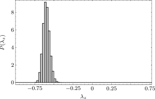
Figure 8: Distribution of the $z$-component of the reduced state operator corresponding to the energy-eigenstates for a completely random perturbation as discussed in section IV.1, 14 particles in C.

Fig. 8 shows the distribution of the values of $\lambda_{z}$ for the complete random interaction discussed in section IV.1. Because the eigenvectors of these Hamiltonians are homogeneously distributed over the unit sphere in the accessible subspace, the $\lambda_{z}$ are narrowly peaked around $-0.6$ Schmidt et al. . Due to the homogeneous distribution of the eigenvectors one expects most of them to contribute to the dynamics with approximately equal weight and therefore $\overline{\mathinner{\langle\hat{\sigma}_{z}\rangle}}$ is expected to be close to the average $\lambda_{z}$.

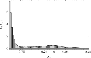
Figure 9: Distribution of the $z$-component of the reduced state operator corresponding to the energy-eigenstates for the spin-star configuration discussed in section IV.2, 14 particles in C.

For the spin-star configuration shown in Fig. 9 the situation is quite different. Although the average over all $\lambda_{z}$ is still $-0.6$, there is a strong peak at $\lambda_{z}=-1$. All the energy eigenstates corresponding to the region $\lambda_{z}\approx-1$ are approximately product states of the form

$$\mathinner{\lvert\varepsilon_{n}\rangle}\approx\mathinner{\lvert 0\rangle}^{\text{S}}\otimes\mathinner{\lvert\chi\rangle}^{\text{C}}$$

with some state $\mathinner{\lvert\chi\rangle}^{\text{C}}$ of the environment (a corresponding peak for eigenstates of the form $\mathinner{\lvert\varepsilon_{n}^{\prime}\rangle}\approx\mathinner{\lvert 1\rangle}^{\text{S}}\otimes\mathinner{\lvert\chi\rangle}^{\text{C}}$ is missing here since this state is not part of the accessible subspace). For the initial condition given by (6) these states do not contribute to the dynamics, therefore the subspace “involved” in the dynamics is only a small fraction of the “accessible” subspace, leading to larger fluctuations in the time evolution. Also the average $\lambda_{z}$ of the contributing states is larger than $-0.6$, therefore the equilibrium temperature differs from its value for a completely random perturbation. The fluctuations could be decreased simply by using a larger environment. However, the average $\lambda_{z}$ of the contributing energy eigenstates, and therefore also the average equilibrium state would not be affected.

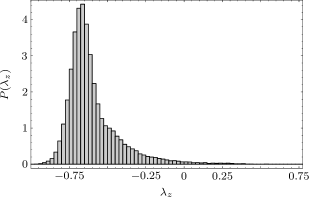
Figure 10: Distribution of the $z$-component of the reduced state operator corresponding to the energy-eigenstates for the ring-star configurations discussed in section IV.3, 14 particles in C.

The shape of the distribution can be changed by introducing intra-environmental coupling. For the types of interaction discussed in the previous section the peak is shifted to larger values of $\lambda_{z}$ for increasing coupling strength, Fig. 10 shows the result for $\gamma=3\alpha$. The distribution is considerably broader than in Fig. 8, while the peak is again close to $\lambda_{z}=-0.6$ and the “involved” subspace is enlarged. Since no large fraction of the energy eigenstates is excluded here by the choice of the initial state, most of the $\lambda_{z}$ contribute and one expects $\overline{\mathinner{\langle\hat{\sigma}_{z}\rangle}}$ to be again close to the average $\lambda_{z}$.

VI “Thermal Duality”: Relaxation to Negative Temperature States

For $k>N/2$ the degeneracy of the environment decreases with energy, $\partial\ln(g^{\text{C}}(E))/\partial{E}<0$, and therefore C can act as an environment imparting a negative absolute temperature to the central spin.

We have shown that the environment leads for the considered subsystem to Schrödinger relaxation approaching a quasi-stationary state with positive temperature (for $k<N/2$). These scenarios may be considered as generic, if simplified, models for what we typically observe in real life. The environments with a finite number of states allow also for a different class of relaxation modes: As a typical consequence of a quantum approach to thermodynamics we find relaxation towards negative temperature states as we replace the accessible environment band index $k$ by $N-k$ (the relaxation behavior of the system is fully symmetrical with respect to the transformation $\mathinner{\lvert s\rangle}\otimes\mathinner{\lvert k,m\rangle}\rightarrow\mathinner{\lvert\bar{s}\rangle}\otimes\mathinner{\lvert N-k,m\rangle}$, where $\bar{s}$ means logical negation)! Contrary to inversion due to optical pumping, these dual states would be dynamically stable just as their positive temperature counterparts. Note, again, that the environment is not a heat bath of negative temperature; in fact, it is far from any canonical state.

Since the population of the energy levels of S at $T<0$ are inverted ($I^{\text{S}}>0$), negative temperatures are actually “hotter” than positive ones. Spin systems and thermodynamics at $T<0$ have been considered before, see e.g. Ramsey (1956); Landsberg (1977). In this regime several statements of thermodynamics, like the second law, have to be reformulated.

Here we show relaxation of S to a state of negative absolute temperature. The situation is the same as discussed in sections III and IV, but now we use $\mathinner{\lvert 0^{\text{S}};k,m^{\text{C}}\rangle}$ and $\mathinner{\lvert 1^{\text{S}};k^{\prime},m^{\text{C}}\rangle}$ with $k=12=N-2$, $k^{\prime}=11=N-3$ (instead of $k=2$, $k^{\prime}=3$) as the accessible subspace for the Schrödinger time evolution (see Fig. 2).

Figure 11: $z$-component of the Bloch vector for the ring-star geometry of section IV.3 with initial state (6) ($N=14$, $k=11$).

Fig. 11 shows $\mathinner{\langle\hat{\sigma}_{z}\rangle}(t)$ for a ring-star geometry of the environment as discussed in section IV.3 and demonstrated in Fig. 5. As expected, the time averaged inversion is close now to $0.6$ instead of $-0.6$. Thus for environments consisting of many spins, the regime $T<0$ can naturally be reached for sufficiently high energy in the environment. In this way it is possible to study quantum thermodynamical effects at negative absolute temperature and possibly even heat conduction between embedded subsystems at temperatures of different sign. This “dual” world, though artificial, may contribute to a better understanding of thermal physics based on quantum mechanics.

VII Conclusion

For the example of a simple subsystem (spin $1/2$) weakly coupled to a spin environment we have shown that the spectral structure of the environment has a strong influence on the decoherence of the central system. We have compared the decoherence of the central spin due to random and structured coupling.

A noninteracting spin environment does not induce relaxation into the local thermal state expected from the band structure, even though energy is the only conserved quantity (the spectrum of the total system is non degenerate). In this case a majority of energy eigenstates do not constitute linear combinations of all states permitted by energy conservation and therefore the accessible part of Hilbert space is considerably reduced for certain non equilibrium initial states like the pure state (6).

By introducing additional mutual coupling within the environment, thus changing its spectrum, some of the properties of the completely random perturbation with respect to relaxation of the central system are restored, provided the coupling strength is adjusted appropriately. By dynamically changing this coupling strength the thermalizing effect of the environment on the central system should be adjustable.

We have concluded our investigation with some explorations on thermal duality: Negative temperatures of the embedded system appear here as a natural consequence of the spectral properties of the environment.

We thank the Landesstiftung Baden-Württemberg for financial support.

References

- Gemmer and Mahler (2003) J. Gemmer and G. Mahler, Eur. Phys. J. B 31, 249 (2003).
- Gemmer et al. (2004) J. Gemmer, M. Michel, and G. Mahler, Quantum Thermodynamics: The Emergence of Thermodynamical Behaviour within Composite Quantum Systems, Springer Lecture Notes in Physics (Springer, 2004).
- Borowski et al. (2003) P. Borowski, J. Gemmer, and G. Mahler, Eur. Phys. J. B 35, 255 (2003).
- Hutton and Bose (2004a) A. Hutton and S. Bose, Phys. Rev. A 69, 042312(7) (2004a).
- Hutton and Bose (2004b) A. Hutton and S. Bose, e-print quant-ph/0408077 (2004b).
- Wang (2002) X. Wang, Phys. Rev. A 66, 034302(4) (2002).
- Briegel and Raussendorf (2001) H. J. Briegel and R. Raussendorf, Phys. Rev. Lett. 86, 910 (2001).
- Vidal et al. (2003) G. Vidal, J. I. Latorre, E. Rico, and A. Kitaev, Phys. Rev. Lett. 90, 227902(4) (2003).
- O’Connor and Wootters (2001) K. M. O’Connor and W. K. Wootters, Phys. Rev. A 63, 052302(9) (2001).
- Breuer et al. (2004) H.-P. Breuer, D. Burgarth, and F. Petruccione, Phys. Rev. B 70, 045323(10) (2004).
- Lages et al. (2004) J. Lages, V. V. Dobrovitski, and B. N. Harmon, e-print quant-ph/0406001 (2004).
- Imamoḡlu et al. (1999) A. Imamoḡlu, D. D. Awschalom, G. Burkard, D. P. DiVincenzo, D. Loss, M. Sherwin, and A. Small, Phys. Rev. Lett. 83, 4204 (1999).
- Makhlin et al. (1999) Y. Makhlin, G. Schön, and A. Shnirman, Nature 398, 305 (1999).
- Diu et al. (1994) B. Diu, C. Guthmann, D. Lederer, and B. Roulet, Grundlagen der Statistischen Physik (de Gruyter, Berlin, 1994).
- Haake (2001) F. Haake, Quantum Signatures of Chaos (Springer, Berlin, 2001), 2nd ed.
- Lieb et al. (1961) E. Lieb, T. Schultz, and D. Mattis, Ann. Phys. (NY) 16, 407 (1961).
- Stollsteimer and Mahler (2001) M. Stollsteimer and G. Mahler, Phys. Rev. A 64, 052301(8) (2001).
- (18) H. Schmidt, J. Gemmer, and G. Mahler, in preparation.
- Ramsey (1956) N. F. Ramsey, Phys. Rev. 103, 20 (1956).
- Landsberg (1977) P. T. Landsberg, J. Phys. A 10, 1773 (1977).