Collective Decoherence of Nuclear Spin Clusters

Abstract

The problem of dipole-dipole decoherence of nuclear spins is considered for strongly entangled spin cluster. Our results show that its dynamics can be described as the decoherence due to interaction with a composite bath consisting of fully correlated and uncorrelated parts. The correlated term causes the slower decay of coherence at larger times. The decoherence rate scales up as a square root of the number of spins giving the linear scaling of the resulting error. Our theory is consistent with recent experiment reported in decoherence of correlated spin clusters.

I Introduction

Quantum information processing devices are expected to be efficient tool for solving some practical problems which are exponentially hard for classical computers Nielsen . Their potential computational performance is achieved by exploiting quantum evolution of many particle system in exponentially large Hilbert space, necessarily including evolution steps through entangled states. Experimental implementation of Shor’s quantum factoring algorithm in seven spin-$1/2$ nuclei molecule have been demonstrated Vandersypen .

The question of whether a scalable implementation of quantum computer is possible in near future implies therefore the question of whether one can protect the fragile entangled states from destructive environment. The dynamics of coherence loss of entangled many-particle clusters has attracted much attention recently. Some authors simulated the noisy environment as a single bosonic bath embracing whole cluster Palma ; Zanardi ; Quiroga ; Hilke . An alternative approach in which the noise sources acting on each cluster constituent are uncorrelated was also studied Quiroga ; additivity . The realistic model of environment will be somewhere between these two cases. Still, the quantitative account for partially correlated environment complicates analysis much Maierle , even for two particle system Storcz . Until recently experimental data on decoherence of large clusters of highly entangled particles were also unavailable. In 2004 the coherence dynamics of groups of up to 650 entangled nuclear spins was observed for the first time Krojanski . This paper is motivated by this experimental breakthrough indicating the partial correlation of the environment.

In this paper, we derive the dependence of decoherence rate of large spin clusters due to completely correlated and uncorrelated perturbation. The results are generalized to the system consisting of nuclear spins $I=1/2$ experimentally studied in the paper Krojanski by using solid-state NMR technique for powdered adamantane samples. Our results show that its dynamics resembles the decoherence due to interaction with a composite bath with a given ratio of correlated and uncorrelated terms. The dependence of decoherence rate on number of spins in the cluster was obtained.

This paper is organized as follows. The investigated system and experimental procedures are described in Sec. II. In Sec. III we calculate the dynamics of NMR signal for the cases of totally correlated/uncorrelated external perturbations and for the experimental situation when decay is caused by internal dipole-dipole interaction. Comparison with experiment data and discussions are given in Sec. IV. Concluding remarks are summarized in Sec. V.

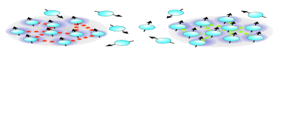
Figure 1: (Color online). Sketch of random array of nuclear spins. Two clusters in partially correlated environments are shown.

II System

Our study was stimulated by the recent results of Krojanski and Suter Krojanski . In their experiments the system of nuclear spins-1/2 (protons) of the powdered admamantane sample was explored by methods of NMR. Initially a system, placed in the external magnetic field $H_{0}$ along $z$ axes, is in thermal equilibrium

$$\rho_{eq}=\frac{\textbf{1}}{2^{N}}+\frac{\gamma\hbar H_{0}}{kT}\sum\limits_{j}{I_{z}^{j}},$$ (1)

where $N$ is number of spins, $\gamma$ is spin gyromagnetic ratio, $k$ is Boltzmann constant, $T$ is temperature and $I^{i}_{z}$ is $z$ component of $i$-th spin operator. With the help of special sequence of radio-frequency pulses Krojanski the high-order correlations between spins grow thereby creating an ensemble of weakly coupled spin clusters. As a result, to describe evolution of spins in the sample it suffices to consider only the dynamics of one such cluster with well defined number of spins $n$ Krojanski ; Baum ; Lacelle .

Existence of high-order coherences in $n$-spin system can be formally described by presence of the off-diagonal elements $\rho_{ij}$ of the spin density operator in any representation whose basis states can be characterized by the total quantum magnetic numbers: $M_{i}|i\rangle=I_{z}|i\rangle$, $M_{j}|j\rangle=I_{z}|j\rangle$. Following the notation used in multiple quantum NMR experiments Slichter we say that every off-diagonal density matrix element $\rho_{ij}$ represents the coherence of the order $M$ where $M=M_{i}-M_{j}$. The number of coherences (different off-diagonal elements) of the order $M$ in $n$-spin system at large $n$ is given by

$$C_{2n}^{n+M}=\frac{{(2n)!}}{{(n-M)!(n+M)!}}\simeq\frac{{2^{2n}}}{{\sqrt{\pi n}}}\exp\left(-\frac{M^{2}}{n}\right).$$ (2)

It is conventional to assume that after long pulse sequence spins are prepared in the state described by the density operator $\rho(0)$ with all even coherences excited with equal probability Baum ; Krojanski .

After the system is prepared in this high-correlated state it decays under dipole-dipole interaction given by the Hamiltonian

$$H_{dd}=\sum\limits_{j<k}d_{jk}\left(3I_{z}^{j}I_{z}^{k}-\bf{I}^{j}\cdot\bf{I}^{k}\right),$$ (3)

where $d_{jk}=\frac{1}{2}\hbar^{2}\gamma^{2}(1-3\cos^{2}[\theta_{jk}])/r_{jk}^{3}$ and $r_{jk}$, $\theta_{jk}$ are corresponding absolute value and the angle with $z$ direction of the vector connecting $j$-th and $k$-th spins.

The system, evolving according to

$$\rho(t)=\exp\left(-\frac{i}{\hbar}H_{dd}t\right)\rho(0)\exp\left(\frac{i}{\hbar}H_{dd}t\right),$$ (4)

does not produce experimentally observable signal. To analyze the effect of dipole-dipole interaction, it undergoes conversion step by another sequence of radio-frequency pulses described in Ref. Baum . During this step multiple-quantum coherences are converted back to single-quantum longitudinal magnetization. After applying a resonant frequency $\pi/2$ pulse which converts the longitudinal magnetization into transverse one the resulting longitudinal magnetization can be determined by measuring the free induction decay. The free induction decay amplitude right after $\pi/2$ pulse is proportional to

$$S(t)\propto{\rm{Tr}}\left[{\rho(t)\rho(0)}\right],$$ (5)

where $t$ is the time the system freely evolved under dipole-dipole Hamiltonian between the end of the preparation step and the beginning of the conversion step. The experiment has to be repeated for sequence of decay times $t$ to obtain the decay of coherence. The overall signal can be presented as a sum of contributions corresponding to different coherence orders $M$ Krojanski

$$S(t)=\sum_{M}S_{M}(t).$$ (6)

The decay times for $S_{M}(t)$ were also measured experimentally Krojanski as a function of coherence order $M$ for different cluster sizes $n$.

III Theory

III.1 Decay of NMR signal due to uncorrelated/correlated external baths

First of all, consider a model when the decay of coherence occurs due to interaction with the external bath. We do not specify the bath itself and use the generic picture. In other words, in this subsection we consider the system without dipole-dipole interaction between spins. Instead we introduce some interaction with external bath which causes the initial spin coherence to decay. In this paper we focus only on the dephasing part of this interaction. A classical analog of such model can be a cluster of spins in fluctuating external magnetic field directed along $z$ axis Maierle .

Henceforward, we use Zeeman basis $|a\rangle=|a_{1}...a_{n}\rangle$, where $a_{i}=\pm 1$ and $I^{i}_{z}|a_{i}\rangle=(a_{i}/2)|a_{i}\rangle$. If we consider the interaction of a single spin with the bath, its evolution in Zeeman basis is given by

$$\rho_{\pm 1,\pm 1}(t)=\rho_{\pm 1,\pm 1}(0);\;\rho_{1,-1}(t)=\rho_{1,-1}(0)e^{-\Gamma(t)},$$ (7)

where we used the interaction representation and the explicit form of the decay function $\Gamma(t)$ is determined by the nature of specific spin-bath interaction. Our main question is how the rate of the collective decoherence of the correlated spin cluster, measured by the technique given in the previous section, differs from the one for the single spin dynamics (7). The answer certainly depends on degree of correlation of the bath at different spin sites.

As the first example, we consider the limiting case of completely uncorrelated environment: each spin interacts with its own bath assuming no correlations between baths related to different spins. In this case the matrix elements of $n$ spin system density operator evolve according to Ref. Palma

$$\rho_{ab}(t)=\rho_{ab}(0)\exp\left(-\Gamma_{ab}(t)\right),$$ (8)

where collective decay function $\Gamma_{ab}(t)$ can be expressed in term of single spin decay function $\Gamma(t)$ as $\Gamma_{ab}(t)=f\Gamma(t)$ and $f=(1/2)\sum_{i}|a_{i}-b_{i}|$ is the Hamming distance between the spin states $|a\rangle$ and $|b\rangle$. The value of Hamming distance $f$ has the same parity as coherence order $M$ and is within the limits $f\in[M,n]$. The number of configurations for given $f$ and $M$ for the system of $n$ spin-1/2 can be found as

$$2^{n-f}C_{n}^{f}C_{f}^{\frac{f+M}{2}}\simeq\frac{2^{2n}}{\pi\sqrt{nf}}\exp\left[-\frac{(f-n/2)^{2}}{n/2}\right]\exp\left[-\frac{M^{2}}{2f}\right].$$ (9)

We can calculate the observable decay of NMR signal $S(t)$ according to (5,8) as

$$S(t)=\sum_{a,b}|\rho_{ab}(0)|^{2}\exp[-\Gamma_{ab}(t)],$$ (10)

where we need to carry out the summation over all possible amplitudes $|\rho_{ab}|$. The signal contributions $S_{M}(t)$ due to certain coherence order $M$ can be evaluated by use of the same formula (10). Although in this case one needs to take the sum over only the subset of configurations $\{|a\rangle\langle b|\}\in\mathfrak{M}$ for whose the additional condition $\sum\nolimits_{j}(a_{j}-b_{j})=2M$ is satisfied. The situation is greatly simplified by assuming that all even coherences are initially excited with equal probability: $|\rho_{ab}(0)|={\rm const}$ if $(1/2)\sum\nolimits_{j}(a_{j}-b_{j})=0,2,4,..$; while all other coherences are not existent $\rho_{ab}(0)=0$ Krojanski ; Baum . We can write

$$S_{M}(t)\propto\sum_{a,b\subset\mathfrak{M}}\exp\left(-if\Gamma(t)\right).$$ (11)

Integrating over all $f$ with corresponding weight (9) we obtain, for $n\Gamma(t)\lesssim 1$, $n\gg 1$ and $M\leq n/2$,

$$S_{M}(t)=\exp\left(-\frac{n}{2}\Gamma(t)\right).$$ (12)

We are interested in times up to $1/e$ decay time where formula (12) is valid. Moreover, since $n\Gamma(t)\lesssim 1$ the decay function is only in the onset regime: $\Gamma(t)\lesssim 1/n\ll 1$ for $n\gg 1$. Therefore, we take only the lowest non-vanishing order of decay function in time (which is always quadratic)

$$\Gamma(t)=\alpha t^{2}+O(t^{4}).$$ (13)

Using (12,13) we obtain

$$S_{M}(t)=\exp\left(-\frac{n}{2}\alpha t^{2}\right).$$ (14)

We emphasize that while we used the short-time expansion for the decay function (13) we expect the formula (14) to be valid up to $1/e$ decay time for the large number of spins $n\gg 1$.

As a second example, we consider the case of completely correlated environment when the whole cluster interacts with the same external bath. The dynamics of the density matrix elements is given by Palma

$$\rho_{ab}(t)=\rho_{ab}(0)\exp\left(-M^{2}\Gamma(t)\right),$$ (15)

and the signal $S_{M}(t)$ decays as

$$S_{M}(t)=\exp\left(-M^{2}\Gamma(t)\right)\simeq\exp\left(-M^{2}\alpha t^{2}\right).$$ (16)

Formula (14) should be compared with (16). Both results show that the decay of signal $S_{M}(t)$ can be approximated by the Gaussian function up to $1/e$ decay times for $n\gg 1$. However, $M$ dependencies for two formulas are totally different. The decay of $S_{M}(t)$ for uncorrelated environment does not demonstrate any dependence on coherence order $M$ while for correlated case it strongly depends on it. Thus, we established the distinctive features of the influence of correlated/uncorrelated environments onto spin cluster dynamics which can be observed experimentally by NMR methods.

III.2 Decay of NMR signal due to internal dipole-dipole interaction

In the experiment by Krojanski and Suter Krojanski the decoherence is caused not by external bath but due to integral dipole-dipole interaction between spins. However, as we show below the resulting behavior of the system can be interpreted with the help of results obtained in the previous subsection.

The dipole-dipole Hamiltonian (3) commutes with Zeeman Hamiltonian

$$H_{Z}=-\gamma\hbar H_{0}\sum_{j}I_{z}^{j}.$$ (17)

However, the complexity of the system and especially the fact that two terms $I_{z}^{j}I_{z}^{k}$ and ${\bf I}^{j}\cdot{\bf I}^{k}$ do not commute makes impossible to find the exact (analytical or numerical) solution of the problem Abragam ; Baum ; Slichter . Existence of high order coherences in the state described by prepared density operator $\rho(0)$ also complicates the application of the traditional method of moments which enables to describe the decay of coherence without solving explicitly for eigenvalues and eigenstates of energy in case of single-quantum NMR experiments VanVleck ; Slichter . In our case the decay of signal is not proportional to the autocorrelation function ${\rm Tr}\{I_{x}(t)I_{x}\}$, as in the case of decay of free induction signal Abragam , but is given by density operator correlator (5) where one needs to evaluate the summation of exponentially large number of terms. In order to obtain the analytical results, we focus on pure dephasing effect of dipole-dipole interaction neglecting any spin exchange between spins that is described by flip-flop term $I_{x}^{j}I_{x}^{k}+I_{y}^{j}I_{y}^{k}$ in Hamiltonian (3). The dipole-dipole dephasing Hamiltonian has the form

$$H_{dd}^{*}=2\sum\limits_{j<k}d_{jk}I_{z}^{j}I_{z}^{k}.$$ (18)

Because dephasing is not associated with energy transfer mechanism it is generally the fastest source of decoherence Mozyrski ; Hu . It becomes the sole process for decoherence in the limit of ”unlike spins” Abragam ; Slichter when spin exchange is suppressed. The consideration of only this type of interaction enables analytical calculations which are also justified by good agreement with experiment in wide range of parameters as it will be demonstrated below.

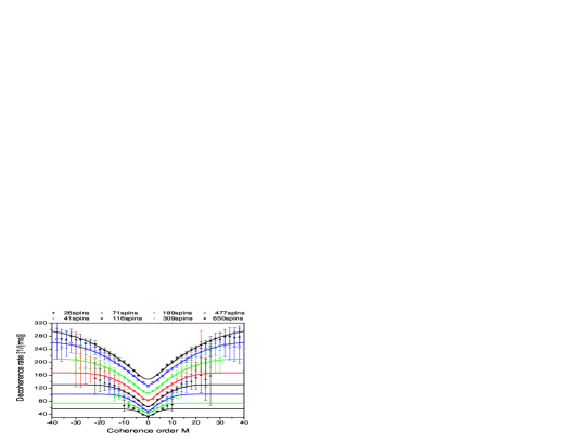
Figure 2: (Color online). Decoherence rate as function of coherence order for different spin cluster sizes. The points represent experimental values Krojanski . The solid lines are obtained with accordance to theoretical formula (23). Degree of correlation $p$ and Van Vleck second moment evaluated from comparison with experiment are given in Table 1.

Table 1: Degree of correlation and second moment for C₁₀H₁₆ obtained from decoherence rates for different cluster sizes.

$n$	26	41	71	116	189	309	477	650
$M_{2}$, $10^{9}$s-2	1.50	1.65	1.60	1.60	1.65	1.60	1.60	1.55
p	0.27	0.28	0.33	0.33	0.32	0.32	0.32	0.32

In the Zeeman representation the off-diagonal density matrix elements evolve according to (8) where decay function is given by

$$\Gamma_{ab}(t)=\frac{it}{2}\sum_{j<k}d_{jk}(a_{j}a_{k}-b_{j}b_{k}).$$ (19)

The dynamics of normalized NMR signal (10) can be analytically expressed as

$$S(t)=16\prod\limits_{j<k}\sum\limits_{a_{l},b_{l}=\pm 1;\atop l\neq k,j}\left|{\rho_{ab}(0)}\right|^{2}{\cos^{2}(\frac{1}{2}d_{kj}t)}.$$ (20)

Exact analytical expression (20) does not provides us with much information yet. Specifically, we intend to obtain explicit dependence on number of spins in the cluster. For this purpose we again assume that all even coherences are initially excited with equal probability and the size of the cluster is large $n\gg 1$ Krojanski ; Baum . After performing some algebra (the details are given in Appendix) we obtain the expression for normalized signal

$$S_{M}(t)=1-pM^{2}\frac{\alpha t^{2}}{2}-(1-p)\frac{n}{2}\frac{\alpha t^{2}}{2}+O(t^{4}),$$ (21)

in the second order in time. Here $\alpha=M_{2}/9$ where $M_{2}=(9/4)\hbar^{-2}\sum_{j}d^{2}_{jk}$ is Van Vleck expression for the second moment Abragam and degree of correlation $p$ is defined as

$$p=\frac{1}{n}\left(\sum\nolimits_{j}d_{jk}\right)^{2}\left/\sum\nolimits_{j}d^{2}_{jk}\right.,$$ (22)

so that $0\leq p\leq 1$. Formula (21) is valid only at short time scales $n\alpha t^{2}\ll 1$, while we are also interested in much larger times up to $n\alpha t^{2}\sim 1$. However, expansion of the signal $S_{M}(t)$ in higher orders in time becomes exceedingly difficult. Therefore, to continue (21) to the longer times we use the analogy with the investigated limiting cases (14, 16). Formula (21) contains two terms proportional to $M^{2}$ and $n/2$ which can be regarded as contributions from correlated and uncorrelated perturbations to spin dynamics, respectively. In fact, the interaction described by Hamiltonian (18) can be semiclassically interpreted as the perturbing magnetic field at the site of each spin (parallel or antiparallel to the strong external magnetic field) produced by all other spins in a cluster. The consequent spread of Larmor frequencies for different spins in the cluster causes destructive interference, or dephasing, observable by the decay of NMR signal. The limit of totally correlated perturbation $p=1$ corresponds to the case $d_{jk}\equiv\rm{const}$ leading to the same perturbing field for each spin in the cluster. In contrast, the case of absolutely random coefficients $\langle d_{jk}\rangle_{j}=0$ gives $p=0$ and fully uncorrelated dynamics. The realistic situation is expected to be in between these two limiting cases. Thus, we write (21) as

$$S_{M}(t)=p\exp\left(-M^{2}\alpha t^{2}\right)+(1-p)\exp\left(-\frac{n}{2}\alpha t^{2}\right),$$ (23)

which is mathematically exact in up to the second order in time but continued to the longer times $n\alpha t^{2}\sim 1$. The total magnetic resonance signal from the cluster $S(t)$ can be obtained by summation over all contributions from different coherence orders $S_{M}(t)$ according to formulas (6) and (23)

$$S(t)=\frac{p}{\sqrt{n\alpha t^{2}+1}}+(1-p)\exp\left(-\frac{n}{2}\alpha t^{2}\right).$$ (24)

In order to understand whether the obtained formulas (23, 24) adequately describe the real experimental situation we should check them with experiment data. The comparison of presented theory and experiment is given in the next section.

IV Comparison of theory with experiment and Discussions

Recent experiments Krojanski allowed us to estimate the degree of correlation parameter for spin clusters in adamantane samples. In Fig. 2 we show curves of decay rates of various coherence orders for different cluster sizes fitted to experimental points. The decoherence rate was defined as the inverse of $1/e$ decay time and was evaluated by solving the algebraic equation $S_{M}(t)=1/e$ where $S_{M}(t)$ is given by formula (23). The degree of correlation $p$ and Van Vleck second moment $M_{2}$ were extracted with the use of MATLAB software by weighted least squares fitting to experimental data for every cluster size $n$. We minimized $\sum_{i}(f(x_{i})-f_{i})^{2}/\Delta_{i}^{2}$ where $x_{i}$ and $f_{i}$ are experimental points, $f(x_{i})$ are corresponding theoretical solutions and $\Delta_{i}$ are experimental errors denoted by vertical bars in Fig. 2. Obtained values of $p$ and $M_{2}$ are given in Table 1. As it follows from formula the definition of second moment VanVleck it is determined by geometrical configurations and do not depend on cluster size $n$. Its moderate fluctuations around average value ($\overline{M}_{2}=(1.60\pm 0.05)\cdot 10^{9}{\rm s^{-2}}$) can be attributed to experimental errors and corrections at small $n$. Obtained values for the second moment are comparable but not identical with the previous theoretical estimates and experimental measured values $M_{2}\simeq 2.6\cdot 10^{9}{\rm s^{-2}}$ for powdered solid adamantane McCall ; Smith . The difference can be explained either by crudity of the chosen model and neglecting flip-flop terms or by discrepancy in the adamantane samples used in different experiments. The question could be resolved by additional measurement of the second moment $M_{2}$ for the given sample.

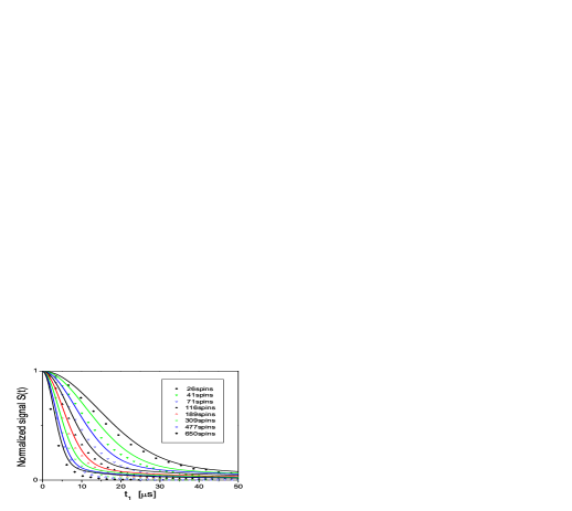
Figure 3: (Color online). Decay of coherence from high-correlated spin clusters for different spin cluster sizes. The points represent experimental values Krojanski . The solid lines are values predicted by formula (24).

Taking the average value of $M_{2}=1.6\cdot 10^{9}{\rm s^{-2}}$ and values for $p$ from Table 1 it is possible to predict the temporal dependence of total NMR signal from high-correlated spin cluster (24) which was measured independently Krojanski for different cluster sizes. The results shown in Fig. 3 are in good agreement with experiment. As can be seen from Fig. 3 the formula (24) describes the initial fast drop of coherence with reasonable accuracy.The divergence at large times between formula (24) (exact up second order in time) and experimental results can be attributed by the contribution of higher order terms.

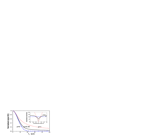
Figure 4: (Color online). Examples of temporal dependence of the signal from high correlated spin cluster with size n=116 and three values of degree of correlation $p$ for perturbation: p=0 (dashed line, uncorrelated perturbation), 0.33 (solid line, partial correlation corresponding to experimental situation), 1 (dotted line, correlated perturbation). The inset shows the decoherence rate as a function of coherence order $M$.

Let us note, that the measured values of decoherence rates for $S_{M}(t)$ give us only one time point in the temporal dynamics of the signal for each value of $M$ and $n$. The parameters $M_{2}$ and $p$ obtained from fitting the solution of $S_{M}(t)=1/e$ to the experimental data allow us to reconstruct the total decay dynamics of $S_{M}(t)$ up to $1/e$ decay times. The following integration over all $M$ provides the decay of overall signal $S(t)$ which was measured independently. This procedure does not, by any means, automatically guarantee the agreement of calculated values of $S(t)$ with experimentally measures ones. The correspondence of theoretical to experimental values demonstrates the good degree of consistency of presented theory.

Formula (24) allows us to analyze the influence of degree of correlation on spin dynamics. Fig. 4 shows the decay of NMR signal for the spin cluster size of intermediate size $n=116$ and three representative examples of degree of correlation $p$: $p=0$ (uncorrelated dynamics), $p=0.33$ (partially correlated dynamics corresponding to the experimental situation) and $p=1$ (correlated dynamics). One can see that initially all three curves decay equally. However, at later times the signal from the spin cluster subject to correlated perturbation exhibits slower decay compared to uncorrelated perturbation. That result comes from the behavior of decoherence rate as function of coherence order $M$. As can be seen from inset of Fig. 4, for uncorrelated perturbation all coherence orders decay with the same, comparatively high, rate $(n\alpha/2)^{1/2}$. In contrast, the decay rate for correlated spin dynamics increases linearly with absolute value of $M$ as $\alpha^{1/2}|M|$. For the most probable configurations, which according to (2) are those with $M\approx 0$, the decay rate for correlated perturbation is actually less than that for uncorrelated perturbation. The fact that correlated environment is acting more delicate on specific groups of states is not surprising. In particular, quantum computing error avoiding schemes based on decoherence free subspaces Zanardi ; Lidar are based on this property.

For implementation of large-scale quantum computation the scaling of decoherence rate with number of qubits is important. From the expression (24) it transpires that decoherence rate of a spin cluster defined as inverse $1/e$ decay time always increases as $\propto\sqrt{n}$ with number of spins $n$ although the corresponding factor depends on degree of correlation $p$. The square root of $n$ scaling was indeed experimentally discovered recently by Krojanski and Suter Krojanski .

For quantum information processing applications it is also important to evaluate the error of a quantum computer, represented by a cluster of high correlated spins, induced by dipole-dipole interaction between spins. The error is defined as deviation of NMR signal from its initial value due to decoherence processes during the time required for elementary gate operation $t_{g}$: $\delta_{n}=1-S(t_{g})$. In order to provide successful implementation of quantum error correction schemes, one needs to maintain this error below the small threshold guarantying fault-tolerance operation of these procedures Nielsen . Taking the smallness of the parameter $\delta_{n}$ into account one can use (24) to obtain

$$\delta_{n}\propto nt^{2}.$$ (25)

This shows that if the error is small it scales linearly with number of spins independently of degree of correlation. The linear scaling of error agrees with theoretical results for bosonic models of environment additivity ; Hilke and suggests that the worst case scenario of ”superdecoherence” Palma is not realized for this particular system.

V Summary

In summary, we have presented a theory of coherence decay of entangled spin clusters states due to internal dipole-dipole interactions. Its dynamics resembles the decoherence due to interaction with a composite bath consisting of fully correlated and uncorrelated parts. The perturbation due to correlated terms leads to the slower decay of coherence at larger times. The decoherence rate scales up as a square root of the number of spins giving the linear scaling of the resulting error. The results obtained can be useful in analysis of decoherence effects in spin-based quantum computers.

Appendix A sdf

The signal contributions $S_{M}(t)$ can be evaluated by use of the formula (10)

$$S_{M}(t)=\sum_{a,b\subset\mathfrak{M}}|\rho_{ab}(0)|^{2}\exp[-\Gamma_{ab}(t)]$$ (26)

Here domain $\mathfrak{M}$ denote all configurations $\left|a\rangle\langle b\right|=\left|a_{1}\ldots a_{n}\rangle\langle b_{1}\ldots b_{n}\right|$ related to the certain coherence order $M$:

$$\sum_{j}(a_{j}-b_{j})=2M.$$ (27)

For every configuration $\left|a\rangle\langle b\right|$ we can divide the total set of $n$ spins into two subsets $\mathbb{E}$ and $\mathbb{N}$,

$$a_{i}=b_{i},\;\forall i\in\mathbb{E};\quad a_{j}=-b_{j},\;\forall j\in\mathbb{N}.$$ (28)

By the use of definitions (28) the decay function $\Gamma_{ab}(t)$ can be simplified as

$$\Gamma_{ab}(t) = i\frac{t}{4}\sum_{j,k}d_{jk}(a_{j}a_{k}-b_{j}b_{k})=i\frac{t}{4}\sum_{j\in\mathbb{E},k\in\mathbb{E}}d_{jk}(a_{j}a_{k}-b_{j}b_{k})+i\frac{t}{4}\sum_{j\in\mathbb{N},k\in\mathbb{N}}d_{jk}(a_{j}a_{k}-b_{j}b_{k})$$ (29)

$$+ i\frac{t}{2}\sum_{j\in\mathbb{E},k\in\mathbb{N}}d_{jk}(a_{j}a_{k}-b_{j}b_{k})=it\sum_{j\in\mathbb{E},k\in\mathbb{N}}d_{jk}a_{j}a_{k}.$$

Assuming that all even coherences are initially excited with equal probability, namely $|\rho_{ab}(0)|={\rm const}$ for all $a,b\in\mathfrak{M}$ (and for all other even order coherences), we obtain the following formula for the decay of $S_{M}(t)$ according to (26,29)

$$S_{M}(t)\propto\sum_{a,b\subset\mathfrak{M}}\exp[-it\sum_{j\in\mathbb{E},k\in\mathbb{N}}d_{jk}a_{j}a_{k}].$$ (30)

We can redistribute the summation in (30) in the following way

$$\sum_{a,b\subset\mathfrak{M}}=\sum_{\mathbb{E},\mathbb{N}}\sum_{a_{j},a_{k}\atop i\in\mathbb{E},k\in\mathbb{N}}.$$ (31)

Here the first sum in the left part of the equation is over all possible choices of subsets $\mathbb{E},\mathbb{N}$ in the set of $n$ spins and second sum is over all possible values of $a_{j},a_{k}$ for $i\in\mathbb{E},k\in\mathbb{N}$. It is easy to see that values $a_{j}$ for $j\in\mathbb{E}$ can take any values $a_{j}=\pm 1$ since they do not contribute to (27) and, therefore, do not change coherence order $M$. We still have the condition for the values $a_{k}$, $k\in\mathbb{N}$:

$$\sum_{k\in\mathbb{N}}a_{k}=M.$$ (32)

Thus, we can evaluate the summation over $a_{j}$ for $j\in\mathbb{E}$ first and obtain

$$S_{M}(t) \propto \sum_{\mathbb{E},\mathbb{N}}\sum_{a_{k},k\in\mathbb{N}}\prod_{j\in\mathbb{E}}\cos(t\sum_{k\in\mathbb{N}}d_{jk}a_{k})$$

$$\propto \sum_{\mathbb{E},\mathbb{N}}\sum_{a_{k},k\in\mathbb{N}}\left(1-\frac{t^{2}}{2}\sum_{j\in\mathbb{E}}(\sum_{k\in\mathbb{N}}d_{jk}a_{k})^{2}+O(t^{4})\right).$$

Now we consider the term $\sum\limits_{j\in\mathbb{E}}(\sum\limits_{k\in\mathbb{N}}d_{jk}a_{k})^{2}$ to express it in terms of parameters of the material. We write

$$d_{jk}=\bar{d}_{j}+\delta_{jk},$$ (34)

where average coupling constant is defined as

$$\bar{d}_{j}=f^{-1}\sum_{k\in\mathbb{N}}d_{jk}.$$ (35)

Here $f$ is Hamming distance between $|a\rangle$ and $|b\rangle$ or the number of spins in subset $\mathbb{N}$. Note, that $\sum_{k\in\mathbb{N}}\delta_{jk}=0$. By use of (32,34) we obtain

$$(\sum_{k\in\mathbb{N}}d_{jk}a_{k})^{2}=(\bar{d}_{j})^{2}M^{2}+\sum_{k\in\mathbb{N}}\delta_{jk}^{2},$$ (36)

where we neglected cross-terms $\sum_{k\in\mathbb{N}}\delta_{jk}a_{k}$ whose contribution is negligible for the large cluster sizes. For $n\gg 1$ we also approximate the summation over subsets by the summation over total cluster with correction to the number of terms in the sum: $\sum_{i}=\left(n/(n-f)\right)\sum_{j\in\mathbb{E}}=(n/f)\sum_{j\in\mathbb{N}}$. These assumptions should lead to the asymptotically correct value of $S_{M}(t)$ for $n\rightarrow\infty$. We then evaluate the the signal decay as

$$S_{M}(t)\propto\sum_{\mathbb{E},\mathbb{N}}\left[1-\frac{t^{2}}{2}\frac{n-f}{n}\left(pM^{2}+(1-p)f\right)\sum_{i}d_{ki}^{2}\right]+O(t^{4}),$$ (37)

where the parameter $p$ is defined as

$$p=\frac{1}{n}\left(\sum\nolimits_{j}d_{jk}\right)^{2}/\sum\nolimits_{j}d^{2}_{jk}.$$ (38)

After integration over all possible $f$ we deduce the closed, analytical form for the signal, exact up to second order in time,

$$S_{M}(t)=1-\frac{t^{2}}{2}\frac{M_{2}}{9}\left(pM^{2}+(1-p)\frac{n}{2}\right)+O(t^{4}),$$ (39)

Here $M_{2}=(9/4)\hbar^{-2}\sum_{j}d^{2}_{jk}$ is Van Vleck expression for the second moment Abragam .

References

- (1) M. Nielsen and I. Chuang, Quantum Computation and Quantum Information (Cambridge University Press, Cambridge, UK, 2000).
- (2) L. M. K. Vandersypen, M. Steffen, G. Breyta, C. S. Yannoni, M. H. Sherwood, and I. L. Chuang, Nature (London) 414, 883 (2001).
- (3) G. M. Palma, K. A. Suominen, and A. K. Ekert, Proc. Roy. Soc. Lond. A 452, 567 (1996).
- (4) P. Zanardi and F. Rossi, Phys. Rev. Lett. 81, 4752 (1998).
- (5) J. H. Reina, L. Quiroga, and N. F. Johnson, Phys. Rev. A 65, 032326 (2002).
- (6) B. Ischi, M. Hilke, and M. Dube, Phys. Rev. B 71, 195325 (2005).
- (7) L. Fedichkin, A. Fedorov, and V. Privman, Phys. Lett. A 328, 87 (2004).
- (8) C. S. Maierle and D. Suter, in Quantum Information Processing, edited by G. Leuchs and T. Beth (Wiley-VCH, Weinheim, 2003), p. 121.
- (9) M. J. Storcz and F. K. Wilhelm, Phys. Rev. A 67, 042319 (2003).
- (10) H. G. Krojanski and D. Suter, Phys. Rev. Lett. 93, 090501 (2004).
- (11) J. Baum, M. Munowitz, A. N. Garroway, and A. Pines, J. Chem. Phys. 83, 2015 (1985).
- (12) S. Lacelle, S. J. Hwang, and B. C. Gerstein, J. Chem. Phys. 99, 8407 (1993).
- (13) A. Abragam, The Principles of Nuclear Magnetism, Clarendon Press, 1983.
- (14) C.P. Slichter, Principles of Magnetic Resonance, Springer-Verlag, 1996.
- (15) J. H. Van Vleck, Phys. Rev. 74, 1168 (1948).
- (16) D. Mozyrsky, Sh. Kogan, V. N. Gorshkov, and G. P. Berman, Phys. Rev. B 65, 245213 (2002)
- (17) X. Hu, R. de Sousa, and S. Das Sarma, cond-mat/0108339.
- (18) D. W. McCall and D. C. Douglass, J. Chem. Phys. 33, 777 (1960).
- (19) G. Smith, J. Chem. Phys. 35, 1134 (1961).
- (20) D. A. Lidar, I. L. Chuang, and K. B. Whaley, Phys. Rev. Lett. 81, 2594 (1998).