Image transfer through a chaotic channel by intensity correlations

Abstract

The three-wave mixing processes in a second-order nonlinear medium can be used for imaging protocols, in which an object field is injected into the nonlinear medium together with a reference field and an image field is generated. When the reference field is chaotic, the image field is also chaotic and does not carry any information about the object. We show that a clear image of the object be extracted from the chaotic image field by measuring the spatial intensity correlations between this field and one Fourier component of the reference. We experimentally verify this imaging protocol in the case of frequency downconversion.

I Introduction

Since the very beginning of its history, second-order ($\chi^{(2)}$) nonlinear optical processes, also called three-wave mixing (TWM), have been used to implement image processing. Initially the process involved was frequency upconversion, namely second-harmonic generation Midwinter68a ; Midwinter68b ; Firester69a ; Firester69b ; Firester69c . Though contemporarily proposed Firester69b ; Firester69c image-processing in downconversion took some more time to be realized Faris94 ; Devaux95a ; Devaux95b ; Devaux95c ; Gavrielides87 ; Avizonis77 ; Lefort96 . The imaging capability of the nonlinear $\chi^{(2)}$ interactions are connected with the spatial properties of the process, which in turn reflect the presence of phase- and frequency-matching conditions among the interacting light fieldsKolobov . In the past years, we have investigated, both theoretically and experimentally, the common features between image processing in TWM and the Gabor holography Gabor49 ; JOSAB00 ; PRA02 ; JOSAB03 , that were first recognized by Firester Firester69a ; Firester69b ; Firester69c . As in an holographic process, TWM imaging protocols require the presence of a reference field, a role that can be played by any of the interacting fields. The generated image thus depends on the simultaneous presence of both the object and the reference fields: this opens the possibility of performing conditional measurements exploiting the correlations between the reference and the image fields. Imaging protocols based on correlations have been used in the quantum domain, in which the generation of couples of entangled photons by spontaneous downconversion and their detection by coincidence techniques Serg_2 , allow to transfer spatial information from one of the twin photons to the other Belin ; Souto_4 ; Serg_1 ; Barbosa . In these protocols, often called ghost imaging, the object is inserted on either signal or idler beyond the crystal. Similar results have been obtained by using a classical source of correlated single-photon pairs Benninck_1 ; Benninck_2 . In the many photon regime, it has been theoretically shown that the same kind of image transfer can be implemented with both quantum entangled Gatti_2 and classically correlated light Cheng ; Gatti_6 ; Magatti . One may alternatively place the object to be imaged on the beam pumping the spontaneous parametric downconversion process Abou . Also in this case, images have been actually detected by mapping suitable photon coincidences between the single-photon pairs in the generated beams Pittman ; Souto_5 ; Souto_6 .

In this paper we exploit the correlation properties intrinsic to $\chi^{(2)}$ processes to recover the image of an object transmitted through a chaotic channel. In fact, if we use a chaotic reference field for the TWM interaction, we obtain the generation of a chaotic image, that does not contain any recognizable information on the original object. Nevertheless, we will demonstrate that by evaluating the intensity correlations between one of the Fourier components of the reference field and the chaotic generated image, we can recover a clean image of the object. As shown in OLinpress , this imaging protocol can be considered a way to simulate many-photon quantum-imaging experiments by using classical fields.

The paper is organized as follows: in Section II we present the analytical description of the imaging process implemented by a $\chi^{(2)}$ interaction in a nonlinear crystal and and experimentally verify the theoretical predictions for a 2-D object; in Section III we show, both analytically and experimentally, how to use the intensity correlations to recover the image of the object in the case of a chaotic seed.

II Image transfer in parametric downconversion

In this Section we present a full 3-D theory of three wave mixing and apply it to the case of a seed field (at $\omega_{1}$) interacting with an intense pump field (at $\omega_{3}>\omega_{1}$). The interaction produces the amplification of seed field and the simultaneous generation of a field at $\omega_{2}=\omega_{3}-\omega_{1}$. This interaction can be used for transferring an amplitude modulation from the pump beam to the generated beam. We demonstrated that this imaging process has holographic properties by showing that, when the amplitude modulation is set by a 3D object, the wavefronts of the generated field reconstruct a 3D image of the objectOL00 . In the experimental paragraph of the Section we verified the theoretical expectations as to location and sizes of the images.

II.1 Theory

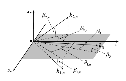
Figure 1: Interaction inside the crystal. The shaded plane contains the optical axis and the normal to the crystal entrance face ($z-$axis).

According to the geometry of Fig. 1, we describe the interaction inside a nonlinear crystal of the following three amplitude-modulated plane-waves, propagating along ${\mathbf{k_{j}}}$

$${\mathbf{E}}_{1}\left({\mathbf{r}},t\right) = \frac{\hat{\mathbf{x}}}{2}\sqrt{\frac{{2\eta_{0}\hbar\omega_{1}}}{{n_{1}}}}\ a_{1}\left({\mathbf{r}}\right)\exp\left(-i{\mathbf{k_{1}}}\cdot{\mathbf{r}}\right)+c.c.$$

$${\mathbf{E}}_{2}\left({\mathbf{r}},t\right) = \frac{\hat{\mathbf{x}}}{2}\sqrt{\frac{{2\eta_{0}\hbar\omega_{2}}}{{n_{2}}}}\ a_{2}\left({\mathbf{r}}\right)\exp\left(-i{\mathbf{k_{2}}}\cdot{\mathbf{r}}\right)+c.c.$$

$${\mathbf{E}}_{3}\left({\mathbf{r}},t\right) = \frac{1}{2}\sqrt{\frac{{2\eta_{0}\hbar\omega_{3}}}{{n_{3}}}}\ \left[\hat{\mathbf{y}}\ a_{3y}\left({\mathbf{r}}\right)+\hat{\mathbf{z}}\ a_{3z}\left({\mathbf{r}}\right)\right]\ \exp\left(-i{\mathbf{k_{3}}}\cdot{\mathbf{r}}\right)+c.c.\ ,$$ (1)

where $n_{j}$ are the refraction indexes, $\eta_{0}$ is the vacuum impedance and the optical frequencies, $\omega_{j}$, satisfy energy matching ($\omega_{3}=\omega_{2}+\omega_{1}$). In the ”slowly varying envelope” approximation, the system describing the second-order interaction inside the crystal is

$${\mathbf{\hat{k}_{1}}}\cdot{\mathbf{\nabla}}a_{1} = i\left[{g_{+}a_{3y}\left({\mathbf{r}}\right)+g_{-}a_{3z}\left({\mathbf{r}}\right)}\right]a_{2}^{*}\left({\mathbf{r}}\right)\exp\left[-i\Delta{\mathbf{k}}\cdot{\mathbf{r}}\right]$$

$${\mathbf{\hat{k}_{2}}}\cdot{\mathbf{\nabla}}a_{2} = i\left[{g_{+}a_{3y}\left({\mathbf{r}}\right)+g_{-}a_{3z}\left({\mathbf{r}}\right)}\right]a_{1}^{*}\left({\mathbf{r}}\right)\exp\left[-i\Delta{\mathbf{k}}\cdot{\mathbf{r}}\right]$$

$${\mathbf{\hat{k}_{3}}}\cdot{\mathbf{\nabla}}a_{3y} = ig_{+}a_{1}\left({\mathbf{r}}\right)a_{2}\left({\mathbf{r}}\right)\exp\left[i\Delta{\mathbf{k}}\cdot{\mathbf{r}}\right]$$

$${\mathbf{\hat{k}_{3}}}\cdot{\mathbf{\nabla}}a_{3y} = ig_{-}a_{1}\left({\mathbf{r}}\right)a_{2}\left({\mathbf{r}}\right)\exp\left[i\Delta{\mathbf{k}}\cdot{\mathbf{r}}\right]\ ,$$ (2)

where $g_{\pm}$ are coupling coefficients Nikogosyan97 and we have defined the phase mismatch vector as $\Delta{\mathbf{k}}=\mathbf{k_{3}}-\mathbf{k_{2}}-\mathbf{k_{1}}$.

In order to analytically solve (2), one of the interacting fields must be taken as non evolving during the interaction: we are interested in the case of non-evolving transverse field $a_{3}\left(\mathbf{r}\right)=a_{3}\left(0\right)$. system (2) becomes

$${\mathbf{\hat{k}_{1}}}\cdot{\mathbf{\nabla}}a_{1} = ig\ a_{3}\left({0}\right)a_{2}^{*}\left({\mathbf{r}}\right)\exp\left[-i\Delta{\mathbf{k}}\cdot{\mathbf{r}}\right]$$

$${\mathbf{\hat{k}_{2}}}\cdot{\mathbf{\nabla}}a_{2} = ig\ a_{3}\left({0}\right)a_{1}^{*}\left({\mathbf{r}}\right)\exp\left[-i\Delta{\mathbf{k}}\cdot{\mathbf{r}}\right]\ ,$$ (3)

where $g$ is a new effective interaction coefficient. The solution of (3) is given by

$$a_{1}\left({\mathbf{r}}\right) = \left\{a_{1}\left(0\right)\left[\cosh\left(Q\frac{\widehat{\Delta\mathbf{k}}}{2}\cdot\mathbf{r}\right)+i\frac{\Delta k}{Q}\sinh\left(Q\frac{\widehat{\Delta\mathbf{k}}}{2}\cdot\mathbf{r}\right)\right]+\right.$$

$$+\left.a_{2}^{*}\left(0\right)\frac{2iga_{3}\left({0}\right)}{\left(\widehat{\Delta\mathbf{k}}\cdot\mathbf{\hat{k}_{1}}\right)Q}\sinh\left(Q\frac{\widehat{\Delta\mathbf{k}}}{2}\cdot\mathbf{r}\right)\right\}\exp\left(-i\frac{\widehat{\Delta\mathbf{k}}}{2}\cdot\mathbf{r}\right)$$

$$a_{2}\left({\mathbf{r}}\right) = \left\{a_{1}^{*}\left(0\right)\frac{2iga_{3}\left({0}\right)}{\left(\widehat{\Delta\mathbf{k}}\cdot\mathbf{\hat{k}_{2}}\right)Q}\sinh\left(Q\frac{\widehat{\Delta\mathbf{k}}}{2}\cdot\mathbf{r}\right)+\right.$$ (4)

$$+\left.a_{2}\left(0\right)\left[\cosh\left(Q\frac{\widehat{\Delta\mathbf{k}}}{2}\cdot\mathbf{r}\right)+i\frac{\Delta k}{Q}\sinh\left(Q\frac{\widehat{\Delta\mathbf{k}}}{2}\cdot\mathbf{r}\right)\right]\right\}\exp\left(-i\frac{\widehat{\Delta\mathbf{k}}}{2}\cdot\mathbf{r}\right)\ ,$$

where

$$Q=\left(\frac{4g^{2}\left|a_{3}\left({0}\right)\right|^{2}}{\left(\widehat{\Delta\mathbf{k}}\cdot\mathbf{\hat{k}_{1}}\right)\left(\widehat{\Delta\mathbf{k}}\cdot\mathbf{\hat{k}_{2}}\right)}-\Delta k^{2}\right)^{1/2}\ .$$ (5)

When the wavevectors satisfy the phase-matching condition ($\Delta\mathbf{k}=0$), solutions (4) become:

$$a_{1}\left({\mathbf{r}}\right) = a_{1}\left(0\right)\cosh\left(\frac{g\left|a_{3}\left({0}\right)\right|}{\mathbf{\hat{b}}\cdot\mathbf{\hat{k}_{1,2}}}\mathbf{\hat{b}}\cdot\mathbf{r}\right)+a_{2}^{*}\left(0\right)\frac{a_{3}\left({0}\right)}{\left|a_{3}\left({0}\right)\right|}\sinh\left(\frac{g\left|a_{3}\left({0}\right)\right|}{\mathbf{\hat{b}}\cdot\mathbf{\hat{k}_{1,2}}}\mathbf{\hat{b}}\cdot\mathbf{r}\right)$$

$$a_{2}\left({\mathbf{r}}\right) = ia_{1}^{*}\left(0\right)\frac{a_{3}\left({0}\right)}{\left|a_{3}\left({0}\right)\right|}\sinh\left(\frac{g\left|a_{3}\left({0}\right)\right|}{\mathbf{\hat{b}}\cdot\mathbf{\hat{k}_{1,2}}}\mathbf{\hat{b}}\cdot\mathbf{r}\right)+a_{2}\left(0\right)\cosh\left(\frac{g\left|a_{3}\left({0}\right)\right|}{\mathbf{\hat{b}}\cdot\mathbf{\hat{k}_{1,2}}}\mathbf{\hat{b}}\cdot\mathbf{r}\right)\$$ (6)

where $\mathbf{b}$ is along the bisector of $\psi$, the angle $\mathbf{\hat{k}_{1}}$-to-$\mathbf{\hat{k}_{2}}$, i.e. $\mathbf{b}=(\mathbf{\hat{k}_{1}}+\mathbf{\hat{k}_{2}})/2$ . Since $\cos\psi$ can be written as

$$\cos\psi=\sin\beta_{1}\sin\beta_{2}+\cos\beta_{1}\cos\beta_{2}\cos\left(\vartheta_{1}-\vartheta_{2}\right)\ ,$$ (7)

we find that $b=\cos(\psi/2)(=\mathbf{\hat{b}}\cdot\mathbf{\hat{k}_{1,2}})$ to be used in (6). Thus $(\mathbf{\hat{b}}\cdot\mathbf{r})/(\mathbf{\hat{b}}\cdot\mathbf{\hat{k}_{1,2}})=f(\vartheta,\beta)r$, where

$$f(\vartheta,\beta)=\frac{\sin\beta_{1}+\sin\beta_{2}+\cos\beta_{1}\sin\vartheta_{1}+\cos\beta_{2}\sin\vartheta_{2}+\cos\beta_{1}\cos\vartheta_{1}+\cos\beta_{2}\cos\vartheta_{2}}{2\cos^{2}\psi/2}\$$ (8)

is a pure geometrical factor. In the following we will consider the particular case of $a_{2}\left(0\right)=0$ and $a_{1}(0)\neq 0$ in the weak-conversion approximation ($g\left|a_{3}\left({0}\right)\right|f(\vartheta,\beta)\ r\ll 1$), for which the solution (6) can be written as

$$a_{1}\left({\mathbf{r}}\right) \simeq a_{1}\left(0\right)$$

$$a_{2}\left({\mathbf{r}}\right) = ig\ f(\vartheta,\beta)\ r\ a_{1}^{*}\left({0}\right)a_{3}\left(0\right)\ ,$$ (9)

that is the amplification of field $a_{1}$ is almost negligible and the generated field $a_{2}$ is linearly dependent on both the pump field $a_{3}$ and the incident field $a_{1}$.

Note that (9) gives the values of the evolved fields at any position ${\mathbf{r}}$ inside the crystal, given a starting point ${\mathbf{r}}=0$ at the entrance face. Different field components starting at different initial points evolve independently and solution (9) can be thus generalized for any transverse field distribution incident on the crystal. In particular, if field $a_{1}(0)$ is a plane wave and the non-evolving pump field $a_{3}(0)$ is amplitude modulated, (9) shows that the modulation is transferred to the generated field $a_{2}$.

II.2 Image formation

We will now explicitly calculate the ”image” field generated on $a_{2}$ given an ”object” field $a_{3}$ in a particular propagation scheme that will be useful for experimental purposes.

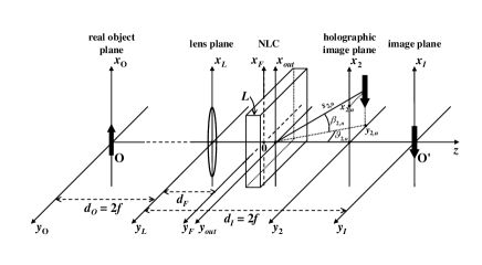
Figure 2: Propagation scheme; NLC, nonlinear crystal.

According to Fig. 2, we consider a modulation of the pump field $a_{3}^{O}(x_{O},y_{O})$ on the object plane $(x_{O},y_{O})$. We insert a converging lens (focal length $f$) on the plane $(x_{L},y_{L})$ located at a distance $d$ from the object plane and at a distance $d_{F}$ from the crystal entrance face, plane $(x_{F},y_{F})$. The field distribution at the entrance face of the crystal in the presence of an infinite ideal lens is given by Goodman88

$$a_{3}\left({\mathbf{r}_{F}}\right) = -\frac{k_{3}^{2}}{4\pi^{2}d_{O}d_{F}}\int\int dx_{O}dy_{O}a_{3}^{O}\left(x_{O},y_{O}\right)\exp\left[-i\frac{k_{3}\left(x_{F}^{2}+y_{F}^{2}\right)}{2d_{F}}\right]\exp\left[-i\frac{k_{3}\left(x_{O}^{2}+y_{O}^{2}\right)}{2d_{O}}\right]$$ (10)

$$\times \int\int dx_{L}dy_{L}\exp\left[-i\frac{k_{3}}{2}\left(\frac{1}{d_{O}}+\frac{1}{d_{F}}-\frac{1}{f}\right)\left(x_{L}^{2}+y_{L}^{2}\right)\right]\exp\left\{-ik_{3}\left[\left(\frac{x_{O}}{d_{O}}+\frac{x_{F}}{d_{F}}\right)x_{L}+\left(\frac{y_{O}}{d_{O}}+\frac{y_{F}}{d_{F}}\right)y_{L}\right]\right\}\ .$$

By evaluating the second integral and letting $d_{O}=2f$ ($2f-2f$ system) we simplify the expression as

$$a_{3}\left({\mathbf{r}_{F}}\right) = \frac{k_{3}}{2\pi id}\exp\left[{i\frac{k_{3}}{2d}\left(x_{F}^{2}+y_{F}^{2}\right)}\right]$$ (11)

$$\times \int dx_{O}dy_{O}a_{3}^{O}\left(x_{O},y_{O}\right)\exp\left[{i\frac{k_{3}}{2d}\frac{f-d}{f}\left(x_{O}^{2}+y_{O}^{2}\right)}\right]\exp\left[{i\frac{k_{3}}{d}\left(x_{F}x_{O}+y_{F}y_{O}\right)}\right]\ ,$$

where $d\equiv 2f-d_{F}$ is the distance between the crystal and the image plane of the lens. We now let the field impinging on each point of the crystal entrance face interact according to (9) by setting $a_{3}\left(0\right)\rightarrow a_{3}\left({\mathbf{r}_{F}}\right)$. According to (1), the spatial amplitude of the generated field ${\mathbf{E}}_{2}$ becomes

$$E_{2}\left({\mathbf{r}_{out}}\right) \propto a_{2}\left({\mathbf{r}_{out}}-{\mathbf{r}_{F}}\right)\exp\left[-i{\mathbf{k_{2}}}\cdot\left({\mathbf{r}_{out}}-{\mathbf{r}_{F}}\right)\right]$$ (12)

$$\propto igrf(\vartheta,\beta)\ a_{1}^{*}(0)\ a_{3}\left({\mathbf{r}_{F}}\right)\exp\left[-i{\mathbf{k_{2}}}\cdot\left({\mathbf{r}_{out}}-{\mathbf{r}_{F}}\right)\right]\ ,$$

being $z_{out}-z_{F}=L$ the crystal depth and $r=|{\mathbf{r}_{out}}-{\mathbf{r}_{F}}|$. In the limit of non-evolving pump, we can take substitute in (12) $a_{3}\left({\mathbf{r}_{F}}\right)$ with $a_{3}\left({\mathbf{r}_{out}}\right)$. Now we let field ${\mathbf{E}}_{2}$ freely propagate from plane $\left(x_{out},y_{out},z_{out}\right)$ to plane $\left(x_{2},y_{2},z_{2}\right)$ along its direction. By neglecting refraction at the crystal interfaces, the field will travel a distance $s_{2}=(z_{2}-z_{out})/(\cos\vartheta_{2}\cos\beta_{2})$ (see Fig. 2). By inserting (11) into (12) and applying free propagation, we get

$$E_{2}\left({\mathbf{r}_{2}}\right) \propto igrf(\vartheta,\beta)\frac{k_{2}}{2\pi is_{2}}\frac{k_{3}}{2\pi id}\ a_{1}^{*}(0)\exp\left[-i\frac{k_{2}\left(x_{2}^{2}+y_{2}^{2}\right)}{2s_{2}}\right]$$ (13)

$$\times \exp\left[-ik_{2}\left(s_{2}+\cos\beta_{2}\cos\vartheta_{2}L\right)\right]\exp\left[ik_{2}\left(\sin\beta_{2}x_{F}+\cos\beta_{2}\sin\vartheta_{2}y_{F}\right)\right]$$

$$\times \int\left\{\int{a_{3}^{O}\left(x_{O},y_{O}\right)\exp\left[{i\frac{k_{3}}{2d}\frac{f-d}{f}\left(x_{O}^{2}+y_{O}^{2}\right)}\right]\exp\left[{i\frac{k_{3}}{d}\left(x_{out}x_{O}+y_{out}y_{O}\right)}\right]dx_{O}dy_{O}}\right\}$$

$$\times \exp\left[-ik_{2}\left(\sin\beta_{2}x_{out}+\cos\beta_{2}\sin\vartheta_{2}y_{out}\right)\right]$$

$$\times \exp\left[i\frac{k_{2}}{s_{2}}\left(x_{2}x_{out}+y_{2}y_{out}\right)\right]\exp\left[i\frac{k_{3}\left(x_{out}^{2}+y_{out}^{2}\right)}{2d}\right]dx_{out}dy_{out}\ .$$

By exchanging the integrations and neglecting the quadratic term inside the last integral we get

$$E_{2}\left({\mathbf{r}_{2}}\right) \propto igrf(\vartheta,\beta)\frac{k_{2}}{2\pi is_{2}}\frac{k_{3}}{2\pi id}\ a_{1}^{*}(0)\exp\left[-i\frac{k_{2}\left(x_{2}^{2}+y_{2}^{2}\right)}{2s_{2}}\right]$$ (14)

$$\times \exp\left[-ik_{2}\left(s_{2}+\cos\beta_{2}\cos\vartheta_{2}L\right)\right]\exp\left[ik_{2}\left(\sin\beta_{2}x_{F}+\cos\beta_{2}\sin\vartheta_{2}y_{F}\right)\right]$$

$$\times \int\left\{\int\exp\left[-i\left(k_{2}\sin\beta_{2}-\frac{k_{2}}{s_{2}}x_{2}-\frac{k_{3}}{d}x_{O}\right)x_{out}-i\left(k_{2}\cos\beta_{2}\sin\vartheta_{2}-\frac{k_{2}}{s_{2}}y_{2}-\frac{k_{3}}{d}y_{O}\right)y_{out}\right]dx_{out}dy_{out}\right\}$$

$$\times a_{3}^{O}\left(x_{O},y_{O}\right)\exp\left[i\frac{k_{3}}{2d}\frac{f-d}{f}\left(x_{O}^{2}+y_{O}^{2}\right)\right]dx_{O}dy_{O}$$

$$= igrf(\vartheta,\beta)\frac{k_{2}}{2\pi is_{2}}\frac{k_{3}}{2\pi id}\ a_{1}^{*}(0)\exp\left[-i\frac{k_{2}\left(x_{2}^{2}+y_{2}^{2}\right)}{2s_{2}}\right]$$

$$\times \exp\left[-ik_{2}\left(s_{2}+\cos\beta_{2}\cos\vartheta_{2}L\right)\right]\exp\left[ik_{2}\left(\sin\beta_{2}x_{F}+\cos\beta_{2}\sin\vartheta_{2}y_{F}\right)\right]$$

$$\times 4\pi^{2}\int\delta\left(k_{2}\sin\beta_{2}-\frac{k_{2}}{s_{2}}x_{2}-\frac{k_{3}}{d}x_{O},k_{2}\cos\beta_{2}\sin\vartheta_{2}-\frac{k_{2}}{s_{2}}y_{2}-\frac{k_{3}}{d}y_{O}\right)$$

$$\times {a_{3}^{O}\left(x_{O},y_{O}\right)\exp\left[{i\frac{k_{3}}{2d}\frac{f-d}{f}\left(x_{O}^{2}+y_{O}^{2}\right)}\right]dx_{O}dy_{O}}$$

$$= igrf(\vartheta,\beta)\frac{k_{2}}{2\pi is_{2}}\ a_{1}^{*}(0)\exp\left[-i\frac{k_{2}\left(x_{2}^{2}+y_{2}^{2}\right)}{2s_{2}}\right]\frac{k_{3}}{2\pi id}$$

$$\times \exp\left[-ik_{2}\left(s_{2}+\cos\beta_{2}\cos\vartheta_{2}L\right)\right]\exp\left[ik_{2}\left(\sin\beta_{2}x_{F}+\cos\beta_{2}\sin\vartheta_{2}y_{F}\right)\right]$$

$$\times 4\pi^{2}\left(\frac{d}{k_{3}}\right)^{2}\int\delta\left(\frac{d}{k_{3}}k_{2}\sin\beta_{2}-\frac{d}{k_{3}}\frac{k_{2}}{s_{2}}x_{2}-x_{O},\frac{d}{k_{3}}k_{2}\cos\beta_{2}\sin\vartheta_{2}-\frac{d}{k_{3}}\frac{k_{2}}{s_{2}}y_{2}-y_{O}\right)$$

$$\times {a_{3}^{O}\left(x_{O},y_{O}\right)\exp\left[{i\frac{k_{3}}{2d}\frac{f-d}{f}\left(x_{O}^{2}+y_{O}^{2}\right)}\right]dx_{O}dy_{O}}$$

$$= -igr\ 4\pi^{2}\left(\frac{d}{k_{3}}\right)^{2}\frac{k_{2}k_{3}}{4\pi^{2}d}\frac{f(\vartheta,\beta)}{s_{2}}\ a_{1}^{*}(0)\exp\left[-i\frac{k_{2}\left(x_{2}^{2}+y_{2}^{2}\right)}{2s_{2}}\right]$$

$$\times \exp\left[-ik_{2}\left(s_{2}+\cos\beta_{2}\cos\vartheta_{2}L\right)\right]\exp\left[ik_{2}\left(\sin\beta_{2}x_{F}+\cos\beta_{2}\sin\vartheta_{2}y_{F}\right)\right]$$

$$\times \exp\left[{i\frac{k_{2}^{2}}{k_{3}s_{2}^{2}}\frac{d(f-d)}{2f}\left[\left(s_{2}\sin\beta_{2}-x_{2}\right)^{2}+\left(s_{2}\cos\beta_{2}\sin\vartheta_{2}-y_{2}\right)^{2}\right]}\right]$$

$$\times a_{3}^{O}\left(\frac{k_{2}}{k_{3}}\frac{d}{s_{2}}\left(s_{2}\sin\beta_{2}-x_{2}\right),\frac{k_{2}}{k_{3}}\frac{d}{s_{2}}\left(s_{2}\cos\beta_{2}\sin\vartheta_{2}-y_{2}\right)\right)$$

$$= -igr\frac{k_{2}}{k_{3}}\frac{d}{s_{2}}f(\vartheta,\beta)\exp\left[i\Phi\left({\mathbf{r}_{2}}\right)\right]\ a_{1}^{*}(0)$$

$$\times a_{3}^{O}\left(\frac{k_{2}}{k_{3}}\frac{d}{s_{2}}\left(s_{2}\sin\beta_{2}-x_{2}\right),\frac{k_{2}}{k_{3}}\frac{d}{s_{2}}\left(s_{2}\cos\beta_{2}\sin\vartheta_{2}-y_{2}\right)\right)\ ,$$

where we have introduced the phase factor $\Phi\left({\mathbf{r}_{2}}\right)$. By writing all the coefficients in a single complex function $C$ we can summarize our result as

$${E}_{2}\left({\mathbf{r}_{2}}\right)=Ca_{1}^{*}(0)a_{3}^{O}\left(\frac{k_{2}}{k_{3}}\frac{d}{s_{2}}\left(\bar{x}_{2}-x_{2}\right),\frac{k_{2}}{k_{3}}\frac{d}{s_{2}}\left(\bar{y}_{2}-y_{2}\right)\right)\ ,$$ (15)

where we have defined

$$\bar{x}_{2}=s_{2}\sin\beta_{2}\ ;\ \bar{y}_{2}=s_{2}\cos\beta_{2}\sin\vartheta_{2}\ .$$ (16)

If we locate the plane $\left(x_{2},y_{2},z_{2}\right)$ so that ${s_{2}\simeq k_{2}/{k_{3}}{d}}$ JOSAB04 , we can simplify the expression as

$${\mathbf{E}}_{2}\left({\mathbf{r}_{2}}\right)=Ca_{1}^{*}(0)a_{3}^{O}\left(\bar{x}_{2}-x_{2},\bar{y}_{2}-y_{2}\right)\ .$$ (17)

The result in (17) shows that with this choice of the propagation configuration, the field distribution on a plane satisfying the holographic relation among the distances is equal to the field distribution on the object plane, provided a double inversion of the coordinates and a shift in position which depends on the propagation direction ${\mathbf{E}}_{1}$. Note that the insertion of the imaging lens on the plane $(x_{L},y_{L})$ was necessary to obtain a real image JOSAB04 .

II.3 Experiment

We experimentally verified the imaging properties of the interaction by using the setup depicted in Fig. 3

The nonlinear crystal was a type I $\beta$-BaB₂O₄ crystal (BBO, cut angle $32^{\mathrm{o}}$, $10$ mm $\times~{}10$ mm $\times~{}4$ mm, Fujian Castech Crystals). The object field was produced by locating on the plane $(x_{O},y_{O})$ a copper sheet with three holes ($\sim 256$ $\mu$m diameter, see inset of Fig. 3) as the mask producing object O. The imaging lens located in the plane $(x_{L},y_{L})$ at a distance $d_{O}=$ 60 cm from the object plane had a focal length $f=300$ mm so as to realize a $2f-2f$ system. The fields ${\mathbf{E}}_{1}$ and ${\mathbf{E}}_{3}$ entering the crystal were obtained from the fundamental ($\lambda_{1}$ = 1064 nm) and the second harmonics ($\lambda_{3}$ = 532 nm) outputs of a Nd:YAG laser (10 Hz repetition rate, $7$-ns pulse duration, Spectra-Physics)thus $\lambda_{2}$ = 1064 nm. The BBO crystal was located at a distance $d_{F}=20$ cm from the lens, so that the image plane of the lens resulted to be at a distance $d=40$ cm beyond the crystal. A system made of a polarizing beam splitter plus a half-wavelength plate was used to obtain a ordinarily polarized field ${\mathbf{E}}_{1}$. For the present experiment, the diffuser D in Fig. 3 was removed from the setup. The sensor of a CCD camera (Dalsa CA-D1-256T, 16 $\mu$m $\times$ 16 $\mu$m pixel area, 12 bits resolution, operated in progressive scan mode) was located in the detection plane $(x_{2},y_{2},z_{2})$. The distance of the CCD from BBO was chosen to be $s_{2}=20$ cm, so as to satisfy $s_{2}=d\ k_{2}/k_{3}$. In Fig. 4 we show the image of the holes as detected by the CCD camera. Note that in agreement with (17) the transverse dimensions of the image were equal to those of the object.

III Chaotic image-transfer in parametric downconversion

In this Section we consider the same interaction seeded by a chaotic field ${\mathbf{E}}_{1}$, which amounts to realize the same image transfer process of above through a chaotic channel. We will demonstrate that in this ”chaotic” situation the imaging system gives no straightforward information on the object. Nevertheless, the intensity fluctuations intrinsic to the chaotic light can be profitably used to implement a protocol for correlated imaging that allows the recovery of the object image.

III.1 Theory

We now suppose that the seed field ${\mathbf{E}}_{1}$ in (1) can be written as an incoherent superposition $N$ plane waves having random complex amplitudes, $a_{1,n}$, and wave vectors, ${\mathbf{k}}_{1,n}$, with random directions but equal amplitudes, $k_{1,n}=2\pi/\lambda_{1}$

$${E}_{1}\left({\mathbf{r}},t\right)\propto\frac{\hat{\mathbf{x}}}{2}\sqrt{\frac{{2\eta_{0}\hbar\omega_{1}}}{{n_{1}}}}\ \sum_{n=1}^{N}a_{1,n}\left({\mathbf{r}}\right)\exp\left(-i{\mathbf{k_{1,n}}}\cdot{\mathbf{r}}\right)\ .$$ (18)

According to solution (9), field ${\mathbf{E}}_{1}$ does not evolve inside the crystal so that its spatial part can be written as ${E}_{1}\left({\mathbf{r}}_{out}\right)\simeq{E}_{1}\left({\mathbf{r}}_{F}\right)$. Due to the chaotic nature of field ${\mathbf{E}}_{1}$, we expect that also its Fourier transform is chaotically distributed. In fact, if we insert a lens of focal length $\tilde{f}$ on the path of field ${\mathbf{E}}_{1}$ at a distance $\tilde{d}$ from the exit plane of the nonlinear crystal, so as to have the Fourier plane on $\left(x_{1},y_{1},z_{1}\right)$ we get

$${E}_{1}\left({\mathbf{r}}_{1}\right) \propto \frac{k_{1}}{2\pi if}\exp\left[-i\frac{k_{1}\left(x_{1}^{2}+y_{1}^{2}\right)}{2\tilde{f}}\left(1-\frac{\tilde{d}}{\tilde{f}}\right)\right]$$ (19)

$$\times \int{{E}_{1}\left({\mathbf{r}}_{out}\right)\exp\left[i\frac{k_{1}}{\tilde{f}}\left(x_{1}x_{out}+y_{1}y_{out}\right)\right]dx_{out}dy_{out}}\ .$$

By substituting the definition of ${\mathbf{E}}_{1}$

$${E}_{1}\left({\mathbf{r}}_{1}\right) \propto \sum_{n=1}^{N}a_{1,n}\frac{k_{1}}{2\pi i\bar{f}}\exp\left[-i\frac{k_{1}\left(x_{1}^{2}+y_{1}^{2}\right)}{2\tilde{f}}\left(1-\frac{\tilde{d}}{\tilde{f}}\right)\right]$$ (20)

$$\times \int\exp\left(-i{\mathbf{k_{1,n}}}\cdot{\mathbf{r}}_{out}\right)\exp\left[i\frac{k_{1}}{\tilde{f}}\left(x_{1}x_{out}+y_{1}y_{out}\right)\right]dx_{out}dy_{out}$$

$$= \sum_{n=1}^{N}C^{\prime}_{n}a_{1,n}\exp\left[-i\frac{k_{1}\left(x_{1}^{2}+y_{1}^{2}\right)}{2\tilde{f}}\left(1-\frac{\tilde{d}}{\tilde{f}}\right)\right]$$

$$\times \delta\left(\frac{k_{1}}{\tilde{f}}(x_{1}-\tilde{f}\sin\beta_{1,n}),\frac{k_{1}}{\tilde{f}}(y_{1}-\tilde{f}\cos\beta_{1,n}\sin\vartheta_{1,n})\right)\ ,$$

which means that if the amplitudes $a_{1,n}$ have random values, the intensity distribution on the plane has the form of a speckle field:

$${I}_{1}\left({\mathbf{r}}_{1}\right)\propto\left|{E}_{1}\left({\mathbf{r}}_{1}\right)\right|^{2}=\sum_{n=1}^{N}\left|C^{\prime\prime}_{n}\right|^{2}\left|{a}_{1,n}\right|^{2}\delta\left(x_{1}-\tilde{f}\sin\beta_{1,n},y_{1}-\tilde{f}\cos\beta_{1,n}\cos\vartheta_{1,n}\right)\ ,$$ (21)

Inside the nonlinear medium, each of the spatial Fourier components of the seed field that is phase matched with the pump field generates an independent contribution to ${\mathbf{E}}_{2}$ according to (9). The overall field at the crystal output face is given by

$${E}_{2}\left({\mathbf{r}}_{out}\right)\propto\sum_{n=1}^{N}igr_{n}f(\vartheta_{n},\beta_{n})a_{1,n}^{*}(0)a_{3}({\mathbf{r}}_{F})\exp\left[-i\ {\mathbf{k}}_{2,n}\cdot\left({\mathbf{r}}_{out}-{\mathbf{r}}_{F}\right)\right]\ ,$$ (22)

where each wavevectors ${\mathbf{k}}_{2,n}$ are assumed to satisfies the phase-matching conditions ${\mathbf{k}}_{3}={\mathbf{k}}_{1,n}+{\mathbf{k}}_{2,n}$. As obvious, this assumption cannot be satisfied for all wavevectors ${\mathbf{k}}_{1,n}$, thus setting an angular limitation to the effectiveness of the interaction. The result (15) can thus be used to evaluate each of the terms in (22) to find the $N$ contributions to field ${\mathbf{E}}_{2}$

$${E}_{2}\left({\mathbf{r}}_{2,n}\right)=C_{n}a_{1,n}^{*}a_{3}^{O}\left(\frac{k_{2}}{k_{3}}\frac{d}{s_{2,n}}\left(\bar{x}_{2,n}-x_{2}\right),\frac{k_{2}}{k_{3}}\frac{d}{s_{2,n}}\left(\bar{y}_{2,n}-y_{2}\right)\right)\ ,$$ (23)

where we have defined

$$\bar{x}_{2,n}=s_{2,n}\sin\beta_{2,n}\ ;\ \bar{y}_{2,n}=s_{2,n}\cos\beta_{2,n}\sin\vartheta_{2,n}\ .$$ (24)

If the effective angular spread of the wavevectors ${\mathbf{k}}_{2,n}$ is not too broad, we can assume that ${s_{2,n}\ \simeq{d}k_{2}/{k_{3}}}$ for all components and that the corresponding $N$ images form on the same plane. Thus from (24) we can write

$${E}_{2}\left({\mathbf{r}}_{2}\right)=\sum_{n=1}^{N}C_{n}a_{1,n}^{*}a_{3}^{O}\left(\bar{x}_{2,n}-x_{2},\bar{y}_{2,n}-y_{2}\right)\ .$$ (25)

Note that also the the field on plane $(x_{2},y_{2},z_{2})$ results to be the sum of $N$ holographic images of the pump field ${\mathbf{E}}_{3}$, reconstructed in $N$ different transverse locations. If we now take into account the random nature of the amplitudes $a_{1,n}$, we obtain that the sum in (25) is as incoherent as that in (18). We can thus write the detected intensity of field $E_{2}$ in the plane $(x_{2},y_{2},z_{2})$ as

$${I}_{2}\left({\mathbf{r}}\right)\propto\left|{E}_{2}\left({\mathbf{r}}_{2}\right)\right|^{2}=\sum_{n=1}^{N}\left|C_{n}\right|^{2}\left|a_{1,n}\right|^{2}\left|a_{3}^{O}\left(\bar{x}_{2,n}-x_{2},\bar{y}_{2,n}-y_{2}\right)\right|^{2}\ ,$$ (26)

This result means that no information about the object field is any more detectable in a direct way. Nevertheless, we can use the correlation properties between fields ${\mathbf{E}_{1}}$ and ${\mathbf{E}_{2}}$ introduced by the nonlinear interaction in the crystal to recover the image of the object. To do this, we select a single position $(x_{1},y_{1})$ in the plane of the Fourier transform of ${\mathbf{E}_{1}}$, that, according to (21), corresponds to choosing a single plane wave having amplitude $a_{1,j}$. We then calculate the correlations of the temporal intensity fluctuations between field ${\mathbf{E}_{1}}$ and field ${\mathbf{E}_{2}}$ we get

$$\langle\Delta{I}_{1}\Delta{I}_{2}\rangle = \langle{I}_{1}{I}_{2}\rangle-\langle{I}_{1}\rangle\langle{I}_{2}\rangle$$ (27)

$$= \langle\left|{a}_{1,j}\right|^{2}\sum_{n=1}^{N}\left|C_{n}\right|^{2}\left|a_{1,n}\right|^{2}\left|a_{3}^{O}\left(\bar{x}_{2,n}-x_{2},\bar{y}_{2,n}-y_{2}\right)\right|^{2}\rangle$$

$$- \langle\left|{a}_{1,j}\right|^{2}\rangle\langle\sum_{n=1}^{N}\left|C_{n}\right|^{2}\left|a_{1,n}\right|^{2}\left|a_{3}^{O}\left(\bar{x}_{2,n}-x_{2},\bar{y}_{2,n}-y_{2}\right)\right|^{2}\rangle$$

$$= \sum_{n=1}^{N}\langle\left|{a}_{1,j}\right|^{2}\left|C_{n}\right|^{2}\left|a_{1,n}\right|^{2}\left|a_{3}^{O}\left(\bar{x}_{2,n}-x_{2},\bar{y}_{2,n}-y_{2}\right)\right|^{2}\rangle$$

$$- \sum_{n=1}^{N}\langle\left|{a}_{1,j}\right|^{2}\rangle\langle\left|C_{n}\right|^{2}\left|a_{1,n}\right|^{2}\left|a_{3}^{O}\left(\bar{x}_{2,n}-x_{2},\bar{y}_{2,n}-y_{2}\right)\right|^{2}\rangle$$

$$= \sum_{n=1}^{N}\left|C_{n}\right|^{2}\left|a_{3}^{O}\left(\bar{x}_{2,n}-x_{2},\bar{y}_{2,n}-y_{2}\right)\right|^{2}\left(\langle\left|{a}_{1,j}\right|^{2}\left|a_{1,n}\right|^{2}\rangle-\langle\left|{a}_{1,j}\right|^{2}\rangle\langle\left|a_{1,n}\right|^{2}\rangle\right)$$

$$= \sum_{n=1}^{N}\left|C_{n}\right|^{2}\left|a_{3}^{O}\left(\bar{x}_{2,n}-x_{2},\bar{y}_{2,n}-y_{2}\right)\right|^{2}\sigma^{2}\left(\left|{a}_{1,n}\right|^{2}\right)\delta_{j,n}$$

$$= \left|C_{j}\right|^{2}\sigma^{2}\left(\left|{a}_{1,j}\right|^{2}\right)\left|a_{3}^{O}\left(x_{2,j}-x_{2},y_{2,j}-y_{2}\right)\right|^{2},$$

where $\sigma^{2}(x)=<x^{2}>-<x>^{2}$ is the variance. In deriving (27) we used the fact that the coefficients $C_{n}$ do not depend on the amplitudes ${a}_{1,n}$ (see (14) and (15)) and that the pump field amplitude $a_{3}$ at each sample of the statistical ensemble. The result in (27) shows that the correlation function between the image on field $E_{2}$ and a single point on the Fourier plane of field $E_{1}$ can reconstruct the image of the object encoded on field $E_{3}$.

III.2 Experiment

For the experimental verification of the results of the previous section, we used the same setup in Fig. 3, modified by introducing the light diffuser $D$ on the seed beam $E_{1}$. The diffuser, a ground-glass wheel, was moved from shot to shot of the laser in order to obtain the temporal statistics needed to evaluate the correlation function (27). A portion of the chaotic field ${\mathbf{E}}_{1}$ emerging from the diffuser was selected with an iris (PH, in Fig. 3) of $\sim$ 8 mm diameter and then filtered in polarization with a polarizing beam splitter, PBS, and a half-wave plate. Lens L₂ ($\tilde{f}=15$ cm) provides the Fourier transform of ${\mathbf{E}}_{1}$ on the plane $(x_{1},y_{1},z_{1})$. The detection planes of $(x_{1},y_{1},z_{1})$ and $(x_{2},y_{2},z_{2})$ were made to coincide on the sensor of the same CCD camera so that each signal occupies half sensor.

First of all, we checked the chaotic nature of both the seed field $E_{1}$ and the generated field $E_{2}$ both in space and in time. A characteristic of chaotic light is to have an intensity obeying thermal distribution, $P(I)=\exp(I/<I>)/<I>$. We thus measured the spatial probability distributions, $P_{\bf r}({I}_{1})$ and $P_{\bf r}({I}_{2})$, of the intensity recorded by the different CCD pixels for a single shot, relative to the Fourier transform of the seed field $E_{1}$ and to the generated field $E_{2}$. Figure 5 shows the results for the spatial distributions along with the intensity maps used to evaluate them (insets). From these results we can see that both the spatial distributions can be fitted by a thermal distribution and that the intensity map relative to the generated field $E_{2}$ has no memory of the field modulation (the same three holes as before) imposed on the pump.

We also measured the temporal (over many repetitions of the laser pulse) probability distributions, $P_{t}({I}_{1})$ and $P_{t}({I}_{2})$, of the intensity recorded by choosing a single pixel of the CCD in the map of $E_{1}$ and $E_{2}$ and recording the intensity values at each laser shot. Also in this case the intensity probability distributions are well fitted by thermal distributions (see Fig. 6). The temporal traces of the intensities of the selected pixels are shown in the insets of the figure.

Once established the correspondence of our experimental setup with the requirements of the theory, we evaluated the correlation function (27) over 1000 shots by taking the whole map $I_{2}\left(x_{2},y_{2}\right)$ and by selecting the value of a single pixel in the intensity map of $I_{1}$.

In Fig. 7 we show the resulting reconstructed image (map of $G\left({I}_{1,j},{I}_{2}(x_{2},y_{2})\right)$): the similarity in the quality of this image compared with that obtained without diffuser (see Fig. 4) is really impressive, in particular if the reconstructed image is compared with any of the single-shot intensity maps $I_{2}\left(x_{2},y_{2}\right)$, see for instance the inset of Fig. 5.

IV Conclusions

In conclusion, we have demonstrated that the spatial intensity correlation properties of the downconversion process can be used to recover a selected image from a chaotic ensemble of holographic images. Note that theoretical results similar to those in Section II.1 and III.1 would be found for any choice of the object and reference fields among the three interacting ones. The image recovered by $G\left({I}_{1,j},{I}_{2}(x_{2},y_{2})\right)$ fulfils the holographic properties of the difference-frequency generated hologram that would be obtained by using the single plane-wave E_1,j as the seed/reference field. We expect that the method also works in the case of an unseeded process, in which no reference field enters the crystal. In this case any twin beam in the parametric fluorescence cone would play the role of our reference and image fields and our intensity correlation protocol should provide an a posteriori selection of a single holographic image. Note that the plane on which this recovered image forms would depend on the choice of the plane-wave component of the twin party used as the reference.

V Acknowledgements

The authors thanks A. Gatti (I.N.F.M., Como) for stimulating discussions, I.N.F.M. (PRA CLON) and the Italian Ministry for University Research (FIRB n. RBAU014CLC$\_$002) for financial support.

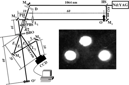
Figure 3: Experimental setup: HS, harmonic separator; D, diffusing plate (removable); M_1-5, mirrors. Lens L₁ images O into O^′ through a $2f-2f$ system. Lens L₂ realizes the Fourier transform of field $E_{1}$ on the CCD sensor. Inset: image taken with an optical microscope of the copper sheet containing the three holes used to produce the object-field modulation. The diameter of the holes was $\sim 200\ \mu$m.

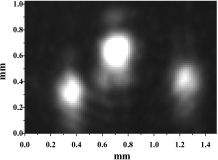
Figure 4: Single-shot holographic image detected in the plane $(x_{2},y_{2},z_{2})$.

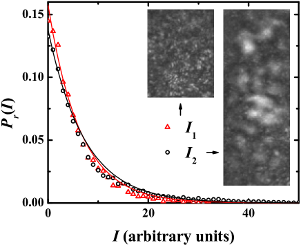
Figure 5: Probability distributions, $P_{\bf r}({I}_{1,2})$ of the intensity recorded by the different CCD pixels for a single shot, relative to the Fourier transform of the seed field $E_{1}$ and to the generated field $E_{2}$. Insets: single-shot intensity maps of $I_{1}$ and $I_{2}$.

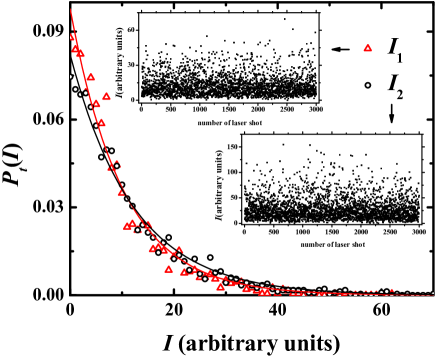
Figure 6: Probability distributions, $P_{t}({I}_{1,2})$ of the intensity of a selected CCD pixel recorded for many successive laser shots. Insets: temporal traces of the intensities.

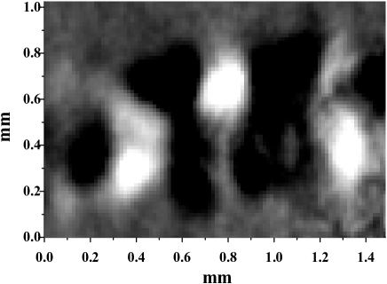
Figure 7: Map of $G\left({I}_{1,j},{I}_{2}(x_{2},y_{2})\right)$ evaluated on 1000 shots

References

• (1) J. E. Midwinter, IEEE J. Quantum Electron. 4 716 (1968).
• (2) J. E. Midwinter, Appl. Phys. Lett. 12 68 (1968).
• (3) A. H. Firester, J. Appl. Phys. 40 4842 (1969).
• (4) A. H. Firester, J. Appl. Phys. 40 4849 (1969).
• (5) A. H. Firester, J. Appl. Phys., 41 703 (1970).
• (6) G. W. Faris and M. Banks, Opt. Letters 19 1813 (1994).
• (7) F. Devaux, E. Lantz, A. Lacourt, D. Gindre, H. Maillotte, P. A. Doreau and T. Laurent, Nonlinear Opt. 11 25 (1995).
• (8) F. Devaux and E. Lantz, Opt. Commun. 114 295 (1995).
• (9) F. Devaux and E. Lantz, Opt. Commun. 118 25 (1995).
• (10) A. Gavrielides, P. Peterson and D. Cardimona J. Appl. Phys. 62 2640 (1987).
• (11) P. V. Avizonis, F. A. Hopf, W. D. Bomberger, S. F. Jacobs, A. Tomita, and K. H. Womack, Appl. Phys. Lett. 31 435 (1977).
• (12) L. Lefort and A. Barthelemy, Opt. Letters 21 848 (1996).
• (13) M. I. Kolobov, Rev. Mod Phys. 71 1539 (1999).
• (14) D. Gabor, Proc. Roy. Soc. A 197 454 (1949).
• (15) A. Andreoni, M. Bondani, Yu. N. Denisyuk and M. A. C. Potenza, J. Opt. Soc. Am. B 17 966 (2000).
• (16) M. Bondani and A. Andreoni, Phys. Rev. A 66, 033805 (2002).
• (17) M. Bondani, A. Allevi and A. Andreoni, J. Opt. Soc. Am. B 20, (2003) 1.
• (18) B. E. A. Saleh, A. F. Abbouraddy, A. V. Sergienko, and M. C. Teich, Phys. Rev. A 62 043816 (2000).
• (19) A. V. Belinskii and D. N. Klyshko, JETP 105 259 (1994).
• (20) P. H. S. Ribeiro, S. Padua, J. C. Machado da Silva and G. A. Barbosa, Phys. Rev. A 49 4176 (1994).
• (21) D. V. Strekalov, A. V. Sergienko, D. N. Klyshko, and Y. H. Shih, Phys. Rev. Lett. 74 3600(1995).
• (22) G. A. Barbosa, Phys. Rev. A 54 4473 (1994).
• (23) R. S. Bennink, S. J. Bentley, and R. W. Boyd, Phys. Rev. Lett. 89 113601 (2002).
• (24) R. S. Bennink, S. J. Bentley, and R. W. Boyd, Phys. Rev. Lett. 92 033601 (2004).
• (25) A. Gatti, E. Brambilla, and L. A. Lugiato, Phys. Rev. Lett. 90 133603 (2003).
• (26) J. Cheng, and S. Han, Phys. Rev. Lett. 92 093903 (2004).
• (27) A. Gatti, E. Brambilla, M. Bache, and L. A. Lugiato, Phys. Rev. A. 70 013802 (2004).
• (28) D. Magatti, F. Ferri, A. Gatti, M. Bache, E. Brambilla, and L. A. Lugiato, arXiv:quant-ph/0408021.
• (29) A. F. Abouraddy, B. E. E. Saleh, A. V. Sergienko, and M. C. Teich, J. Opt. Soc. Am. B 19 1174 (2002).
• (30) T. B. Pittman, Y. H. Shih, D. V. Strekalov, and A. V. Sergienko, Phys. Rev. A 52 R3429 (1995).
• (31) C. H. Monken, P. H. S. Ribeiro, and S. Padua, Phys. Rev. A 57 3123 (1998).
• (32) D. P. Caetano, P. H. S. Ribeiro, J. T. C. Pardal, and A. Z. Khoury, Phys. Rev. A 68 023805 (2003).
• (33) E. Puddu, A. Allevi, A. Andreoni and M. Bondani, Chaotic imaging in frequency downconversion, Opt. Letters. In press.
• (34) Yu. N. Denisyuk, A. Andreoni, M. Bondani and M. A. C. Potenza, Opt. Letters 25 890 (2000).
• (35) J. W. Goodman, Introduction to Fourier Optics (Mc Graw-Hill, New York 1988).
• (36) V. G. Dmitriev, G. G. Gurzadyan and D. N. Nikogosyan, Handbook of Nonlinear Optical Crystals (Springer, Berlin-Heidelberg-New York 1997).
• (37) B. E. A. Saleh and M. C. Teich, Fundamentals of Photonics (J. Wiley & Sons, New York 1991).
• (38) M. Bondani, A. Allevi, A. Brega, E. Puddu and A. Andreoni, J. Opt. Soc. Am. B 21 280 (2004).
Refer to caption