Classical Capacity of
Quantum Binary Adder Channels

Abstract

We analyze the quantum binary adder channel, i.e. the quantum generalization of the classical, and well–studied, binary adder channel: in this model qubits rather than classical bits are transmitted. This of course is as special case of the general theory of quantum multiple access channels, and we may apply the established formulas for the capacity region to it. However, the binary adder channel is of particular interest classically, which motivates our generalizing it to the quantum domain. It turns out to be a very nice case study not only of multi–user quantum information theory, but also on the role entanglement plays there. It turns out that the analogous classical situation, the multi–user channel supported by shared randomness, is not distinct from the channel without shared randomness, as far as rates are concerned. However, we discuss the effect the new resource has on error probabilities, in an appendix.

We focus specially on the effect entanglement between the senders as well as between senders and receiver has on the capacity region. Interestingly, in some of these cases one can devise rather simple codes meeting the capacity bounds, even in a zero–error model, which is in marked difference to code construction in the classical case.

I Classical and quantum
binary adder channels

The binary adder channel is a popular and well–studied example of a multiple access channel in classical information theory: $L$ senders may each choose a bit $x_{i}\in\{0,1\}$, which results in the receiver getting

$$y=x_{1}+\ldots+x_{L}\in\{0,\ldots,L\}.$$

I.e., the receiver can have only very limited information on the sent bits: e.g. if $y=1$ she knows that exactly one $x_{i}$ equals $1$, the others being $0$, but has no information on $i$. It is easily seen that this channel (which remarkably is deterministic) is equivalent to the channel randomly permuting the bits $(x_{1},\ldots,x_{L})$: in one direction, from such a random permutation the receiver can still calculate the sum $y$ of the bits, thus simulating the output of the former channel. In the other direction, $y$ can be used to generate a uniform distribution on the words $(x_{1},\ldots,x_{L})$ with weight $y$, which is a simulation of the latter channel.

The general expression for the capacity region of multiple access channels, as determined by Ahlswede [1, 2], can be evaluated explicitly (see e.g. [12]), and gives for the two–user case $L=2$ (to which we shall restrict our attention for the moment) the achievable rate pairs $(R_{1},R_{2})$ of non–negative reals $R_{1}$, $R_{2}$ with

$$R_{1},R_{2}\leq 1,\quad R_{1}+R_{2}\leq\frac{3}{2},$$ (1)

for asymptotic block coding. This result is obtained by random coding arguments and it is still an open problem to construct codes achieving these bounds. Especially the zero–error case received much attention, and we refer to the survey [19], and to [3] as the most recent contribution. There is also a literature on low–error codes: see e.g. [18].

The above reasoning on the adder channel makes it plausible to define the quantum binary adder channel as follows: it has inputs $L$ qubits, i.e. states on two–dimensional Hilbert spaces ${\cal H}_{\ell}\simeq{\mathbb{C}}^{2}$, $\ell=1,\ldots,L$, and acts as random permuter of these qubits (for thoughts on the general methodology of quantum information theory we refer the reader to [8]). Formally, define for a permutation $\pi\in S_{L}$ the permuting operators on ${\cal H}=\bigotimes_{\ell=1}^{L}{\cal H}_{\ell}$ by

$$F_{\pi}:{|{\psi_{1}}\rangle}\otimes\cdots\otimes{|{\psi_{L}}\rangle}\longmapsto{|{\psi_{\pi(1)}}\rangle}\otimes\cdots\otimes{|{\psi_{\pi(L)}}\rangle},$$

and let the adder channel $\alpha$ be the following completely positive, trace preserving (c.p.t.p.) map on ${\cal B}({\cal H})$:

$$\alpha: \sigma \longmapsto\frac{1}{L!}\sum_{\pi\in S_{L}}F_{\pi}\sigma F_{\pi}^{*}$$

$$\sigma_{1}\otimes\cdots\otimes\sigma_{L} \longmapsto\frac{1}{L!}\sum_{\pi\in S_{L}}\sigma_{\pi(1)}\otimes\cdots\otimes\sigma_{\pi(L)}.$$

To send classical information via this channel the senders will choose input qubits to their systems, while the receiver will choose a measurement, described by a positive operator valued measure (POVM). For example the senders could choose to send only states from the fixed basis ${|{0}\rangle},{|{1}\rangle}\in{\mathbb{C}}^{2}$, and the receiver performing the von Neumann measurement consisting of the projectors

$${{|{x_{1}\ldots x_{L}}\rangle}\!{\langle{x_{1}\ldots x_{L}}|}}={{|{x_{1}}\rangle}\!{\langle{x_{1}}|}}\otimes\cdots\otimes{{|{x_{L}}\rangle}\!{\langle{x_{L}}|}}.$$

This obviously reproduces the behaviour of the classical adder channel, making $\alpha$ a generalization of the former.

However, we shall be concerned also with the effect of entanglement on the transmission capacity of this channel: in this case we assume that the senders and the receiver share initially some multipartite entangled state, and sending information is by the senders modifying their respective share of this state ${|{\iota}\rangle}\in\bigotimes_{\ell=1}^{L}{\cal K}_{\ell}\otimes{\cal H}_{R}$ by applying quantum operations (i.e., c.p.t.p. maps) and subsequently putting it into $\alpha$.

The details of these procedures are discussed more precisely below, but we can remark that the channel proposed is an example of a quantum multiple access channel: the first who appeared to have discussed the model are Allahverdyan and Saakian [5]. The capacity region in full was determined in [25] (the result being reproduced in [17] for the particular case of pure signal states), in the model of product state encodings (i.e. the same condition under which the Holevo bound holds and is achieved with single–user channels [16]). The result, for the two–sender case to which we shall restrict ourselves from here on, is as follows: Suppose user $1$ may take actions $i\in{\mathcal{I}}$, user $2$ actions $j\in{\mathcal{J}}$, which results in the (possibly mixed) output state $W_{ij}$ on Hilbert space ${\cal H}$. This is a very general description of a quantum multiple access channel, which obviously includes the ones discussed above (with or without entanglement). We assume that the channel acts memoryless, meaning that in $n$ uses of the channel, with inputs $i^{n}=i_{1}\ldots i_{n}\in{\mathcal{I}}^{n}$ and $j^{n}=j_{1}\ldots j_{n}\in{\mathcal{J}}^{n}$ the output state will be

$$W^{n}_{i^{n}j^{n}}=W_{i_{1}j_{1}}\otimes\cdots\otimes W_{i_{n}j_{n}}\text{ on }{\cal H}^{\otimes n}.$$

An $(n,\lambda)$–block code for this channel is defined as a triple $(f_{1},f_{2},D)$, with two functions

$$f_{1}: \ {\cal M}_{1}\longrightarrow{\mathcal{I}}^{n},$$

$$f_{2}: \ {\cal M}_{2}\longrightarrow{\mathcal{J}}^{n},$$

(${\mathcal{M}}_{1}$, ${\mathcal{M}}_{2}$ being finite sets of messages), and a decoding POVM $D=\left(D_{m_{1}m_{2}}\right)_{m_{i}\in{\mathcal{M}}_{i}}$, such that the (average) error probability

$$\begin{split}e&(f_{1},f_{2},D)\\ &\phantom{==}=1-\frac{1}{|{\mathcal{M}}_{1}||{\mathcal{M}}_{2}|}\sum_{m_{i}\in{\mathcal{M}}_{i}}\!{\operatorname{Tr}}\!\left(W^{n}_{f_{1}(m_{1})f_{2}(m_{2})}D_{m_{1}m_{2}}\right)\end{split}$$

is at most $\lambda$. The capacity region ${\bf R}$ is then defined as the set of all pairs $(R_{1},R_{2})$ such that there exist $(n,\lambda)$–block codes with the error probability $\lambda$ tending to zero, and the code rates tending to $R_{1}$ and $R_{2}$, respectively, as $n\rightarrow\infty$:

$$\frac{1}{n}\log|{\mathcal{M}}_{1}|\longrightarrow R_{1},\quad\frac{1}{n}\log|{\mathcal{M}}_{2}|\longrightarrow R_{2}.$$

Note that in this paper $\log$ is the logarithm to basis $2$.

We will assume that ${\cal H}$ is finite, so we might take ${\mathcal{I}}$, ${\mathcal{J}}$ to be finite, too. However, allowing general measure spaces and measures $P$ on ${\mathcal{I}}$, $Q$ on ${\mathcal{J}}$, and a measurable map $W$ does not change the result, but allows greater flexibility.

Theorem 1

Denote by ${\bf R}_{PQ}$ the set of points $(R_{1},R_{2})\in{\mathbb{R}}^{2}$ such that $R_{1},R_{2}\geq 0$ and

$$R_{1} \leq I(P;W|Q),$$

$$R_{2} \leq I(Q;W|P),$$

$$R_{1}+R_{2} \leq I(P\times Q;W).$$

Then the capacity region of the channel is given by the closed convex hull of the union of the ${\bf R}_{PQ}$. ∎

Here the information terms are quantum, as follows:

$$I(R;W)=H\left(\int dR(ij)W_{ij}\right)-\int dR(ij)H(W_{ij}),$$

with the von Neumann entropy $H$, and

$$I(P;W|Q)=\int dQ(j)I(P;W_{\cdot j}),$$

where $W_{\cdot j}$ is the single–user classical–quantum channel conditional on $j$:

$$W_{\cdot j}:i\longmapsto W_{ij},$$

and likewise $W_{i\cdot}$ and $I(Q;W|P)$.

Observe the formal analogy of this formula to the classical case, where there appear mutual information and conditional mutual information, too [1, 2].

We will use this formula to prove in the sequel (section III) that the capacity region of $\alpha$, with no entanglement available, coincides with the region for the classical two–adder channel, described by eq. (1). This we shall take as the final piece of evidence that our definition really represents the quantum generalization of the classical adder channel. Then we add entanglement to our investigation: in section IV the enlargement of the capacity region due to entanglement between the senders is investigated, while we allow sender–receiver entanglement in section V, increasing the capacity region once more, the latter effect of course being reminiscent of dense coding [10]. To explain, however, the increase of the capacity due to entanglement between the senders, we have to understand the particular kind of correlation provided by it: in this direction, we discuss in the appendix the easy fact that shared randomness between all of the parties does not increase the capacity region of the classical adder channel (in fact, this is even true for the quantum adder channel $\alpha$). So, the observed increase of the capacity has to be attributed to quantum effects.

To end this introduction, a few words on previous and related work: in [17], final section, some remarks regarding entanglement between the users are made. However, as this paper is only concerned with the pure state case of multiple access coding, there is no overlap with the present work.

Two further works have come to our attention that touch upon the peculiar “interference” (mutual disturbance) between messages in a multiple access channel, both in a situation where previous entanglement between two senders and the receiver is assumed, and a noiseless channel is considered (instead of our noisy random permuter): In [14], rather unaware of the information theoretic meaning, the case of 1–ebit of sender–receiver entanglement in the form of a GHZ–state is treated, in a noiseless setting: in section 3.2. of that work it is shown that the rate–sum $3$ is optimal. There is overlap with this work concerning the idea of generalized superdense coding, compare subsection V-A.

In [21] this investigation is carried to $d$–level $N$–party higher GHZ–states, and coding methods meeting the capacity region bounds (which can be derived from theorem 1) are discussed.

II Two–user quantum adder channel

These are the channels we are going to investigate in the sequel:
Fix an initial pure state ${|{\iota}\rangle}$ of the system ${\cal H}_{1}\otimes{\cal H}_{2}\otimes{\cal H}_{R}$, where ${\cal H}_{1}={\cal H}_{2}={\mathbb{C}}^{2}$ are the two users’ qubit systems (with fixed orthonormal basis ${|{0}\rangle}$, ${|{1}\rangle}$), and ${\cal H}_{R}$ is the receiver’s system (one may obviously assume that ${\cal H}_{R}={\mathbb{C}}^{4}$, as the initial state is always pure). As sets of allowed actions we define all local quantum operations:

$${\mathcal{I}}={\mathcal{J}}=\{\varphi:{\cal B}({\mathbb{C}}^{2})\rightarrow{\cal B}({\mathbb{C}}^{2})|\varphi\text{ c.p.t.p.}\}.$$

The channel $\alpha$ for two senders has the simple form

$$\alpha:\sigma\longmapsto\frac{1}{2}\left(\sigma+F\sigma F^{*}\right),$$

with the flip operator

$$F=F_{(12)}:{|{u}\rangle}\otimes{|{v}\rangle}\longmapsto{|{v}\rangle}\otimes{|{u}\rangle}.$$

Notice that a most convenient eigenbasis of this unitary is provided by the Bell states

$${|{\Phi^{+}}\rangle} =\frac{1}{\sqrt{2}}({|{00}\rangle}+{|{11}\rangle}),$$

$${|{\Phi^{-}}\rangle} =\frac{1}{\sqrt{2}}({|{00}\rangle}-{|{11}\rangle}),$$

$${|{\Psi^{+}}\rangle} =\frac{1}{\sqrt{2}}({|{01}\rangle}+{|{10}\rangle}),$$

$${|{\Psi^{-}}\rangle} =\frac{1}{\sqrt{2}}({|{00}\rangle}+{|{11}\rangle}),$$

the first three (which span the symmetric subspace ${\cal S}$) with phase $+1$, the last with phase $-1$. From this one can see that the effect of $\alpha$ is to destroy coherence between ${\cal S}$ and ${\mathbb{C}}{|{\Psi^{-}}\rangle}$: it is equivalent to an incomplete nondemolition von Neumann measurement of the projector onto ${\cal S}$ and its complement ${{|{\Psi^{-}}\rangle}\!{\langle{\Psi^{-}}|}}$.

The swap super–operator for density operators is defined as follows: for a density operator $\sigma$ on ${\mathbb{C}}^{2}\otimes{\mathbb{C}}^{2}$ let

$$S(\sigma)=F\sigma F^{*}.$$

This means that the channel “quantum binary adder with prior entanglement ${|{\iota}\rangle}$” is described by mapping $f\in{\mathcal{I}}$, $g\in{\mathcal{J}}$ to the output state

$$W_{fg}=\frac{1}{2}\bigl{(}f\otimes g\otimes{\operatorname{id}}({{|{\iota}\rangle}\!{\langle{\iota}|}})+(S\otimes{\operatorname{id}})(f\otimes g\otimes{\operatorname{id}}({{|{\iota}\rangle}\!{\langle{\iota}|}}))\bigr{)}.$$

Making indistinguishable permutations of the input qubits surely is a necessary requirement for a candidate quantum adder channel, as well as reducing to the classical binary adder for the particular choice of input bases and output measurement (both of which $\alpha$ satisfies). Notice however that $\alpha$ even keeps coherence in the symmetric subspace ${\cal S}$. Just as well one could destroy it by doing a nondemolition measurement in this or some other basis after $\alpha$. Nevertheless, apart from being hard to motivate (which basis to choose?), this is an unnecessary “classicalisation” of the channel: as we shall see in the next section our definition of quantum adder channel has the same capacity region as the classical adder channel. We might take this as saying that $\alpha$ is the “most quantumly” channel generalizing the usual binary adder channel and at the same time not increasing the capacity region.

III No entanglement

Here we treat the case of a trivial receiver’s system ${\cal H}_{R}={\mathbb{C}}$, and ${|{\iota}\rangle}={|{00}\rangle}$. Thus coding amounts to independent choices of states ${|{\phi}\rangle}$ and ${|{\psi}\rangle}$, and ${\mathcal{I}}$, ${\mathcal{J}}$ may be identified with the sets of pure states on ${\cal H}_{1},{\cal H}_{2}$, respectively (note that choosing mixed states to encode is obviously suboptimal here). We will show that the capacity region in this case is identical to the classical adder channel’s. To do this, we obviously have only to prove that our quantum channel obeys the same upper rate bounds as the classical one (because the classical coding schemes work identically for the quantum channel).

Because the individual bounds on $R_{1}$ and $R_{2}$ are convex combinations of quantities trivially upper bounded by $1$, we have only to show that $R_{1}+R_{2}\leq 3/2$, which in turn will follow if we show that

$$I(P\times Q;W)\leq\frac{3}{2},$$

for all distributions $P$ and $Q$ on the pure qubit states. In more extensive writing this means

$$\begin{split}H&\!\left(\int\!\!dP(\phi)dQ(\psi)\frac{1}{2}({{|{\phi}\rangle}\!{\langle{\phi}|}}\!\otimes\!{{|{\psi}\rangle}\!{\langle{\psi}|}}+{{|{\psi}\rangle}\!{\langle{\psi}|}}\!\otimes\!{{|{\phi}\rangle}\!{\langle{\phi}|}})\right)\\ &-\int\!\!dP(\phi)dQ(\psi)H\!\left(\!\frac{1}{2}({{|{\phi}\rangle}\!{\langle{\phi}|}}\!\otimes\!{{|{\psi}\rangle}\!{\langle{\psi}|}}+{{|{\psi}\rangle}\!{\langle{\psi}|}}\!\otimes\!{{|{\phi}\rangle}\!{\langle{\phi}|}})\!\right)\\ &\phantom{============================}\leq\frac{3}{2}.\end{split}$$ (2)

It is an easy exercise to show that for two vectors ${|{v}\rangle},{|{w}\rangle}$ with $t=|{\langle{v}|}w\rangle|$, one has

$$H\left(\frac{1}{2}({{|{v}\rangle}\!{\langle{v}|}}+{{|{w}\rangle}\!{\langle{w}|}})\right)=H\left(\frac{1-t}{2},\frac{1+t}{2}\right),$$ (3)

with the Shannon entropy of a binary distribution at the right hand side.

Applied to the terms in the second integral in eq. (2) we get

$$H\!\left(\!\frac{1}{2}({{|{\phi}\rangle}\!{\langle{\phi}|}}\!\otimes\!{{|{\psi}\rangle}\!{\langle{\psi}|}}+{{|{\psi}\rangle}\!{\langle{\psi}|}}\!\otimes\!{{|{\phi}\rangle}\!{\langle{\phi}|}})\!\right)=H\!\left(\!\frac{1\pm|{\langle{\phi}|}\psi\rangle|^{2}}{2}\!\right)\!.$$

Introducing

$$\rho_{P}=\int dP(\phi){{|{\phi}\rangle}\!{\langle{\phi}|}},\quad\rho_{Q}=\int dQ(\psi){{|{\psi}\rangle}\!{\langle{\psi}|}}$$

we can rewrite the left hand side of eq. (2) as

$$\begin{split}H&\left(\frac{1}{2}\rho_{P}\otimes\rho_{Q}+\frac{1}{2}\rho_{Q}\otimes\rho_{P}\right)\\ &\phantom{======}-\int dP(\phi)dQ(\psi)H\left(\frac{1\pm|{\langle{\phi}|}\psi\rangle|^{2}}{2}\right).\end{split}$$ (4)

Now an important observation comes in: the function $H\left(\frac{1\pm x}{2}\right)$, for $0\leq x\leq 1$, is strictly concave and strictly decreasing, with value $1$ at $x=0$ and value $0$ at $x=1$. In particular

$$H\left(\frac{1-x}{2},\frac{1+x}{2}\right)\geq 1-x.$$

But Taylor expansion shows even more:

$$1-x^{2}\leq H\left(\frac{1-x}{2},\frac{1+x}{2}\right)\leq 1-\frac{1}{2}x^{2}.$$ (5)

Plugging this in we can lower bound the subtraction term in eq. (4) by

$$1-\int dP(\phi)dQ(\psi)|{\langle{\phi}|}\psi\rangle|^{2}=1-{\operatorname{Tr}}(\rho_{P}\rho_{Q}).$$

Thus we get an upper bound on the left hand side of eq. (2):

$$H\left(\frac{1}{2}\rho_{P}\otimes\rho_{Q}+\frac{1}{2}\rho_{Q}\otimes\rho_{P}\right)-1+{\operatorname{Tr}}(\rho_{P}\rho_{Q}).$$ (6)

The maximum of this expression is obtained when $\rho_{P}$ and $\rho_{Q}$ commute, in fact if they are equal: replacing both $\rho_{P}$ and $\rho_{Q}$ by $\frac{1}{2}(\rho_{P}+\rho_{Q})$ increases both the entropy contribution (because of subadditivity), and the trace contribution:

$${\operatorname{Tr}}\left(\frac{\rho_{P}+\rho_{Q}}{2}\right)^{2}-{\operatorname{Tr}}\rho_{P}\rho_{Q}={\operatorname{Tr}}\left(\frac{\rho_{P}-\rho_{Q}}{2}\right)^{2}\geq 0.$$

But with commuting $\rho_{P}$, $\rho_{Q}$ the situation is essentially the classical one, and we are done. More precisely, $P=Q$ may be taken as distribution on a common eigenbasis ${|{0}\rangle},{|{1}\rangle}$ of $\rho_{P}=\rho_{Q}$, in which case the maximum in eq. (6) is easily seen to be attained at $\rho_{P}=\frac{1}{2}{\leavevmode\hbox{\small 1\normalsize\kern-3.30002pt1}}$: when $\rho_{P}=\rho_{Q}$ the expression in eq. (6) becomes

$$2H(\rho)-1+{\operatorname{Tr}}\left(\rho^{2}\right).$$

In terms of $\rho$’s eigenvalues $(1\pm y)/2$ this reads, and can be estimated, as

$$2H\left(\frac{1-y}{2},\frac{1+y}{2}\right)+\frac{y^{2}-1}{2}\leq\frac{3}{2}-\frac{1}{2}y^{2},$$

the latter clearly obtaining the maximum at $y=0$.

Observe that in this case only $\langle\phi{|{\psi}\rangle}=0$ or $=1$ occur with positive probability in eq. (4), so in eq. (6) we have in fact equality: the points in this region can be achieved by using the classical input states ${|{0}\rangle},{|{1}\rangle}$, the corresponding POVM $\bigl{(}{{|{xy}\rangle}\!{\langle{xy}|}}:x,y\in\{0,1\}\bigr{)}$ followed by a classical postprocessing (decoding). Observe that we cannot, however, provide explicit code constructions to do this, as was pointed out in the introduction.

IV Sender–sender entanglement

Up to basis change the most general two–qubit (pure) state that can be shared among the senders is

$${|{\iota}\rangle}=\alpha{|{00}\rangle}+\beta{|{11}\rangle},$$

with $\alpha\geq\beta\geq 0$ and $\alpha^{2}+\beta^{2}=1$.

Before we go into the general case, we consider the two extremes:

1. No entanglement: $\alpha=1$ (meaning no entanglement) was treated in the previous section, and the capacity region determined.

2. Maximal entanglement: on the other hand, for $\alpha=\beta=1/\sqrt{2}$ (maximal entanglement), the upper bounds from theorem 1 are trivially bounded by $2$, each; $R_{1},R_{2},R_{1}+R_{2}\leq 2$. As it turns out, this is the capacity region. For example, the corner $(2,0)$ is achieved by sender two sending nothing, while sender one modulates ${|{\iota}\rangle}$ as in dense coding. Note that the four Bell–states are invariant under the channel, so the $2$ bits encoded by sender one are recovered without error. This is a notable feature, as we pointed out the difficulty of finding error–free codes for the unassisted adder channel.

Now we approach the general case: one strategy which seems to be good is to (asymptotically reversibly!) concentrate the $n$ copies of the state ${|{\iota}\rangle}$ into $k=nH(\alpha^{2},\beta^{2})-o(n)$ many EPR pairs [7]. Then use time sharing between $k$ uses of the maximal entanglement scheme (item 2 above) and $n-k$ uses of the no entanglement scheme (item 1 above), resulting in an achievable rate region cut out by the inequalities

$$R_{1},R_{2} \leq 2\cdot H(\alpha^{2},\beta^{2})+1\cdot\bigl{(}1-H(\alpha^{2},\beta^{2})\bigr{)}$$

$$=1+H(\alpha^{2},\beta^{2}),$$ (7)

$$R_{1}+R_{2} \leq 2\cdot H(\alpha^{2},\beta^{2})+\frac{3}{2}\cdot\bigl{(}1-H(\alpha^{2},\beta^{2})\bigr{)}$$

$$=\frac{3}{2}+\frac{1}{2}H(\alpha^{2},\beta^{2}).$$ (8)

The right hand side of eq. (IV), $1+H(\alpha^{2},\beta^{2})$ is easily seen to be actually an upper bound on any achievable individual rate: indeed, let the second sender cooperate optimally, by sending all his entanglement to the receiver. Then, even disregarding the channel noise, the maximal entanglement between the first sender and the receiver is $nH(\alpha^{2},\beta^{2})$, and it is fairly easy to show that under these circumstances sending $n$ qubits (again disregarding the noise) can transmit at most an asymptotic rate of $1+H(\alpha^{2},\beta^{2})$ classical bits [6, 26].

In view of this, we also conjecture that the right hand side of eq. (IV), $\frac{3}{2}+\frac{1}{2}H(\alpha^{2},\beta^{2})$, is always an upper bound on the rate sum. A proof of this, however, has eluded us so far.

V Sender–receiver entanglement

We shall study two cases of entanglement between senders and receiver, both distinguished by their symmetry: the case of a shared GHZ–state in subsection V-A, and the case of maximal entanglement in subsection V-B.

V-A 1 ebit

Here the parties share initially a GHZ–state

$${|{\iota}\rangle}=\frac{1}{\sqrt{2}}({|{000}\rangle}+{|{111}\rangle}).$$

Note that this is the unique three–qubit state (up to local unitaries) having all its single particle states equal to the maximally mixed state.

Now, we shall prove that the region described by the inequalities

$$R_{1},R_{2}\leq 2,\quad R_{1}+R_{2}\leq\frac{5}{2},$$

is indeed the full capacity region: the individual rate bounds are obvious again, so we have only to bound the rate–sum.

We begin again with considering the unitary case: Let the users employ unitaries

$$U_{a}=\left(\begin{array}[]{rr}\alpha&-\overline{\beta}\\ \beta&\overline{\alpha}\end{array}\right),\quad U_{b}=\left(\begin{array}[]{rr}\gamma&-\overline{\delta}\\ \delta&\overline{\gamma}\end{array}\right).$$

(Global phases do not matter). With the flip unitary $F$ from above, it is a straightforward calculation to obtain

$$\begin{split}\left|{\langle{\iota}|}U_{a}^{*}\otimes U_{b}^{*}\otimes{\leavevmode\hbox{\small 1\normalsize\kern-3.30002pt1}}(F\otimes{\leavevmode\hbox{\small 1\normalsize\kern-3.30002pt1}})U_{a}\otimes U_{b}\otimes{\leavevmode\hbox{\small 1\normalsize\kern-3.30002pt1}}{|{\iota}\rangle}\right|&=|{\langle{0}|}U_{a}^{*}U_{b}{|{0}\rangle}|\\ &=|{\langle{1}|}U_{a}^{*}U_{b}{|{1}\rangle}|.\end{split}$$

Thus we can estimate (with $T_{ab}=U_{a}\otimes U_{b}\otimes{\leavevmode\hbox{\small 1\normalsize\kern-3.30002pt1}}$)

$$\begin{split}&R_{1}+R_{2}\\ &\phantom{/}\leq\!H\!\!\left(\int\!\!dP(a)dQ(b)\frac{1}{2}\bigl{(}T_{ab}{{|{\iota}\rangle}\!{\langle{\iota}|}}T_{ab}^{*}\!+\!S\otimes{\operatorname{id}}(T_{ab}{{|{\iota}\rangle}\!{\langle{\iota}|}}T_{ab}^{*})\!\bigr{)}\!\!\right)\\ &\phantom{==========}-\int\!dP(a)dQ(b)H\!\left(\frac{1\pm|{\langle{0}|}U_{a}^{*}U_{b}{|{0}\rangle}|}{2}\right)\\ &\phantom{/}\leq\!H\!\!\left(\int\!\!dP(a)dQ(b)\frac{1}{2}\bigl{(}T_{ab}{{|{\iota}\rangle}\!{\langle{\iota}|}}T_{ab}^{*}\!+\!S\otimes{\operatorname{id}}(T_{ab}{{|{\iota}\rangle}\!{\langle{\iota}|}}T_{ab}^{*})\!\bigr{)}\!\!\right)\\ &\phantom{==========}-1+\int\!dP(a)dQ(b)|{\langle{0}|}U_{a}^{*}U_{b}{|{0}\rangle}|^{2},\end{split}$$

where we have used eq. (5). We will employ the following important inequality:

Lemma 2

For a general state $\rho$ on the composite system ${\cal H}_{1}\otimes{\cal H}_{2}$ and a POVM $(E_{1},\ldots,E_{n})$ on ${\cal H}_{2}$, it holds for the measurement probabilities $\lambda_{i}={\operatorname{Tr}}\bigl{(}\rho({\leavevmode\hbox{\small 1\normalsize\kern-3.30002pt1}}\otimes E_{i})\bigr{)}$ and the post–measurement states

$$\sigma_{i}=\frac{1}{\lambda_{i}}\left(\sqrt{{\leavevmode\hbox{\small 1\normalsize\kern-3.30002pt1}}\otimes E_{i}}\right)\rho\left(\sqrt{{\leavevmode\hbox{\small 1\normalsize\kern-3.30002pt1}}\otimes E_{i}}\right)$$

that

$$H(\rho)\leq H(\lambda_{1},\ldots,\lambda_{n})+\sum_{i=1}^{n}\lambda_{i}H(\sigma_{i}).$$

Proof  . Defining

$$\rho_{i}=\frac{1}{\lambda_{i}}\sqrt{\rho}\bigl{(}{\leavevmode\hbox{\small 1\normalsize\kern-3.30002pt1}}\otimes E_{i}\bigr{)}\sqrt{\rho},$$

one has $\rho=\sum_{j}\lambda_{j}\rho_{j}$, and $H(\rho_{j})=H(\sigma_{j})$ for all $j$: in fact $\rho_{j}$ and $\sigma_{j}$ are conjugate operators via a unitary, by the polar decomposition. Finally, by the data processing inequality [4]

$$H(\lambda)\geq H(\rho)-\sum_{j}\lambda_{j}H(\rho_{j}),$$

and we are done. $\Box$

We apply this to the complete measurement in the basis $\{{|{0}\rangle},{|{1}\rangle}\}$ on the receiver’s system ${\cal H}_{R}$, and obtain:

$$\begin{split}&R_{1}+R_{2}\leq\\ &\phantom{=}1\!+\!\sum_{k=0}^{1}\frac{1}{2}\left[H\!\Bigg{(}\!\int\!dP(a)dQ(b)\frac{1}{2}\Big{(}U_{a}\!\otimes\!U_{b}{{|{kk}\rangle}\!{\langle{kk}|}}U_{a}^{*}\!\otimes\!U_{b}^{*}\right.\\ &\phantom{==============:}\left.+S(U_{a}\!\otimes\!U_{b}{{|{kk}\rangle}\!{\langle{kk}|}}U_{a}^{*}\!\otimes\!U_{b}^{*})\Big{)}\Bigg{)}\right.\\ &\phantom{============:}-1+\int dP(a)dQ(b)|{\langle{k}|}U_{a}^{*}U_{b}{|{k}\rangle}|^{2}\Bigg{]}\!.\end{split}$$

Each of the two terms corresponding to $k=0,1$ can be written in the form

$$\begin{split}H&\left(\int d\tilde{P}(\phi)d\tilde{Q}(\psi)\frac{1}{2}({{|{\phi}\rangle}\!{\langle{\phi}|}}\otimes{{|{\psi}\rangle}\!{\langle{\psi}|}}+{{|{\psi}\rangle}\!{\langle{\psi}|}}\otimes{{|{\phi}\rangle}\!{\langle{\phi}|}})\right)\\ &\phantom{==============}-1+\int d\tilde{P}(\phi)d\tilde{Q}(\psi)|\langle\phi{|{\psi}\rangle}|^{2}.\end{split}$$

Since this — by the reasoning of section III — is bounded by $3/2$, we get the desired bound $R_{1}+R_{2}\leq 5/2$.

Now we demonstrate how, utilizing a code for the classical adder channel, the points in the region

$$R_{1},R_{2}\leq 2,\quad R_{1}+R_{2}\leq\frac{5}{2}$$

can be achieved. For this, let an $n$–block code for the classical binary adder channel be given, with rates $R_{1}$ and $R_{2}$. This code can be used to encode using the initial GHZ–state: instead of sending a bit $b$ each sender applies $\sigma_{x}^{b}$. It is easily seen that by a C–NOT of his share of ${|{\iota}\rangle}$ onto the other two qubits he receives through the channel and measuring in the standard basis the receiver obtains exactly the same data as in the classical case with the classical adder code.

However, this still allows sender one (say) to encode an extra bit into the phase: she either applies $\sigma_{z}$ or $1$ on her part of ${|{\iota}\rangle}$, thus either leaving the joint state in the subspace

$${\cal P}={\rm span}\left\{\frac{1}{\sqrt{2}}({|{ab0}\rangle}+{|{\overline{a}\overline{b}1}\rangle}):a,b\in\{0,1\}\right\},$$

or steering it isometrically into the orthogonal subspace

$${\cal N}={\rm span}\left\{\frac{1}{\sqrt{2}}({|{ab0}\rangle}-{|{\overline{a}\overline{b}1}\rangle}):a,b\in\{0,1\}\right\}.$$

Note that both these subspaces are stable under the channel and that the named $\sigma_{z}$ action commutes with it. So, the receiver can decode the extra bit first, by distinguishing first ${\cal P}$ and ${\cal N}$ by a nondemolition measurement (then rotating back into ${\cal P}$ if need be) and then proceeding as just described with the classical code. This achieves the rate point $(1+R_{1},R_{2})$. Equally, we can achieve the point $(R_{1},1+R_{2})$, proving our claim.

V-B 2 ebits — maximal entanglement

The general form of an entangled state between the users’ systems and the receiver’s is

$$\begin{split}{|{\iota}\rangle}&=\alpha_{0}{|{\Phi^{+}}\rangle}\otimes{|{u_{0}}\rangle}+\alpha_{1}{|{\Phi^{-}}\rangle}\otimes{|{u_{1}}\rangle}\\ &\phantom{=}+\alpha_{2}{|{\Psi^{+}}\rangle}\otimes{|{u_{2}}\rangle}+\alpha_{3}{|{\Psi^{-}}\rangle}\otimes{|{u_{3}}\rangle}.\end{split}$$

This to have maximal entanglement it is necessary and sufficient that $\alpha_{i}=1/2$ for all $i$, and the $u_{i}$ are orthonormal vectors.

In this case the general upper bounds for $R_{1},R_{2}$ are dominated by $R_{1},R_{2}\leq 2$, so again we only have to estimate the rate–sum $R_{1}+R_{2}$: first, for unitary actions $U_{1}$, $U_{2}$ of both users, the resulting state $U_{1}\otimes U_{2}{{|{\iota}\rangle}\!{\langle{\iota}|}}U_{1}^{*}\otimes U_{2}^{*}$ is still maximally entangled, hence the output state is an equal mixture of

$$\frac{1}{2}({|{\Phi^{+}}\rangle}\otimes{|{v_{0}}\rangle}+{|{\Phi^{-}}\rangle}\otimes{|{v_{1}}\rangle}+{|{\Psi^{+}}\rangle}\otimes{|{v_{2}}\rangle}\pm{|{\Psi^{-}}\rangle}\otimes{|{v_{3}}\rangle}),$$

for an orthonormal system $v_{0},\ldots,v_{3}$. Its von Neumann entropy is, by equation (3), equal to $H\left(\frac{1}{4},\frac{3}{4}\right)$. Thus, if both users are restricted to unitary codings, we find

$$R_{1}+R_{2}\leq 4-H\left(\frac{1}{4},\frac{3}{4}\right)\approx 3.189,$$

and the bound can be achieved by taking the normalized Haar measure for either user, or — more discretely — the uniform distribution on the Pauli unitaries (including 11) for either user. Note that again, like in the case of the classical adder channel, we cannot give an explicit good code, nor is it obvious to produce optimal zero–error codes: our argument relies on the random coding in the general coding theorem 1.

V-C Significance of our findings

To begin with, comparing the rate regions described so far, we see that they increase as we go from no entanglement, via partial to maximal sender–sender entanglement, and further as we increase the sender–receiver entanglement. There are, however, two important caveats to consider before concluding that the capacity region increases with the available entanglement (apart from only conjecturing eq. (IV) to be the optimal bound on the rate sum for partial sender–sender entanglement):

First, we have in both scenarios considered in section V assumed that the encoding is done using unitaries. Though we don’t expect non–unitary operations to perform better (as they introduce further noise) we lack a proof of that statement.

Second, we have on occasions (sections III and V) only considered single–copy maximisation of the involved informations. As was pointed out in the beginning the outer bounds on the capacity region apply in general only if the signal states allowed in coding are products. This is satisfied in all situations under investigation here if the encoding operations (unitary or general) are products themselves.

The situation may change if arbitrary encodings on blocks are allowed (as maybe for the single–user channel: this relates to the additivity of the Holevo capacity of a channel (see [23]). It is quite conceivable that the analysis of section III will not apply any longer. The same holds for the entanglement–assisted situations: only in a case like maximal entanglement in section IV the bounds are so simple that they obviously still apply here.

We would like to point out that the problem of determining the capacity region in the presence of entanglement (in particular to find out if it increases at all beyond the separable encoding region discussed above) is not contained in the analogous discussion of [25]: this is another and more general instance of the extended additivity question for the classical capacity of quantum channels, discussed in [26]: notice that in the discussion there, as in the case of section III above, the sender input states of their choosing into the channel, while in the presence of entanglement they input quantum operations.

VI The case of many senders

Let us now turn to an investigation of the analogous problem for $L>2$ senders, each sharing an ebit with the receiver initially:

$${|{\Phi}\rangle}=2^{-L/2}\sum_{x_{1},\ldots,x_{L}}{|{x_{1}}\rangle}\otimes\cdots\otimes{|{x_{L}}\rangle}\otimes{|{x_{1}\ldots x_{L}}\rangle}_{R}.$$

Instead of aiming at finding the whole capacity region of the $L$–user quantum binary adder channel, we will concentrate on a quantity of particular interest for symmetric channels like this one: the maximal rate sum $\Sigma R=R_{1}+\ldots+R_{L}$. We remind the reader that for a classical binary adder channel this is maximized by $L$ uniform input distributions, for which $\Sigma R$ becomes the entropy of a binomial distribution, and $\Sigma R\sim\frac{1}{2}\log L$ for large $L$ [11].

For the entanglement–assisted quantum case, consider for the moment a scheme where each user modulates her share of the entangled state ${|{\Phi}\rangle}$ with a Pauli operator, uniformly chosen at random from $\{{\leavevmode\hbox{\small 1\normalsize\kern-3.30002pt1}},\sigma_{x},\sigma_{y},\sigma_{z}\}$. Because these can always be commuted through to acting on $R$, all signal states of this channel are (up to local unitaries on the receiver system) equivalent to

$$\tau:=\frac{1}{L!}\sum_{\pi}(F_{\pi}\otimes{\leavevmode\hbox{\small 1\normalsize\kern-3.30002pt1}}){{|{\Phi}\rangle}\!{\langle{\Phi}|}}(F_{\pi}^{*}\otimes{\leavevmode\hbox{\small 1\normalsize\kern-3.30002pt1}}),$$

and the average output is maximally mixed on $2L$ qubits. To evaluate the Holevo information in the bound for the rate sum, we thus have to calculate the entropy of the state $\tau$.

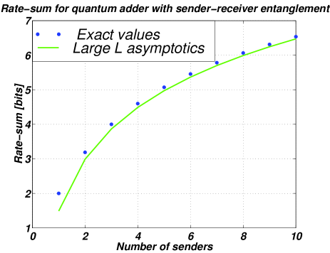
Figure 1: Achievable rate sum for the quantum binary adder channel with maximal prior entanglement between senders and receiver. The dots are the exact values from eq. (9), while the line is the asymptotics of these values for large $L$, $\Sigma R\sim\frac{3}{2}\log L$.

Since $\tau$ is an average over the symmetric group, we write it in terms of the Clebsch–Gordan decomposition of $({\mathbb{C}}^{2})^{\otimes L}$ into irreducible decompositions of $U(2)$ and $S_{L}$ [24]:

$$({\mathbb{C}}^{2})^{\otimes L}=\bigoplus_{k=0}^{\lfloor L/2\rfloor}{\cal S}_{k}\otimes{\cal P}_{k},$$

with the ($U(2)$, irreducible) spin representations ${\cal S}_{k}$ of dimension $L-2k+1$, and the ($S_{L}$, irreducible) permutation representations ${\cal P}_{k}$ of dimension $d_{k}={L\choose k}\!-\!{L\choose{k-1}}$.

Hence, by writing ${|{\Phi}\rangle}$ in this decomposition for both sender and receiver system, and applying Schur’s lemma,

$$\tau=\bigoplus_{k=0}^{\lfloor L/2\rfloor}p_{k}{{|{\Phi_{k}}\rangle}\!{\langle{\Phi_{k}}|}}_{{\cal S}_{k}{\cal S}_{k}}\otimes\frac{1}{d_{k}}{\leavevmode\hbox{\small 1\normalsize\kern-3.30002pt1}}_{{\cal P}_{k}}\otimes\frac{1}{d_{k}}{\leavevmode\hbox{\small 1\normalsize\kern-3.30002pt1}}_{{\cal P}_{k}},$$

with some maximally entangled state ${|{\Phi_{k}}\rangle}$ on ${\cal S}_{k}\otimes{\cal S}_{k}$. From counting dimensions, we can calculate the (probability!) weights in this sum: $p_{k}=d_{k}(L-2k+1)2^{-L}$, and we get,

$$\Sigma R=2L-H\bigl{(}p_{0},\ldots,p_{\lfloor L/2\rfloor}\bigr{)}-\sum_{k=0}^{\lfloor L/2\rfloor}p_{k}\log\bigl{(}d_{k}^{2}\bigr{)}.$$ (9)

For $L=2$ we recover our result from section V-B, which gives rate sum $\approx\!3.189$; for $L=3$ and $4$, this formula gives values $4$ and $\approx\!5.057$, respectively. For large $L$, we can quite straightforwardly see that $\Sigma R\sim\frac{3}{2}\log L$. The plot in figure 1 illustrates the result.

VII Concluding remarks

We have introduced and studied the quantum binary adder channels, determining its capacity region in the case of two senders, without prior entanglement and with the help of various three–party entangled states between the senders and the receiver. It turned out that sender–sender entanglement already increases the capacity region (and that this region is indeed directly related to the amount of entanglement available), to become even larger for sender–receiver entanglement, which we studied in two important cases: a GHZ–state and maximal entanglement (2 ebits).

For a large number $L$ of users, we found that maximal sender–receiver entanglement almost triples the achievable rate sum compared the classical adder channel. Though we didn’t prove it, it seems likely that our figure actually is also best possible.

Among questions that deserve further study we would like to advertise two as specially interesting: First, as the case of “much entanglement” in our case study proved extremely fruitful, we are motivated to ask about the entanglement assisted capacity region of a quantum multiple access channel, in the spirit of the beautiful work [9], where the classical capacity of a quantum channel was studied in the presence of arbitrary entanglement. Second, we propose the problem of finding the rates of quantum information transmission via the quantum adder channel, and more generally for an arbitrary quantum multiple access channel, which lies out of the scope of the present investigation.

Appendix: Shared randomness in
multiuser information theory

The classical analogue of entanglement between the communication parties is shared randomness. Does this additional resource change capacity regions?

As it turns out, the answer is “no”: the reason being that the use of shared randomness can be described as (jointly) randomly using several ordinary communication protocols. Also, in multiuser situations we favour the average error concept (average error probabilities over assumed uniform distribution on all message sets) over the familiar maximal error concept in single–user situations. Hence, if we are given a code with shared randomness and all its $K$ (average) error probabilities bounded by $\epsilon$, there is one of the constituent ordinary codes with average error probabilities bounded by $K\epsilon$. Observe that $K$ is a constant of the setup, e.g. the number of senders in the multiple–access channel.

So, allowing the use of shared randomness does not increase the capacity regions.

However, to conclude that shared randomness is no good, would be premature. Indeed, as we will indicate here, one of its uses may be to turn the awkward average error performance into maximal error bounds. This is something nontrivial — in contrast to the case of single–sender coding where the two concepts are essentially equivalent —, for it is known that the maximal error concept can yield strictly smaller capacity regions than the average error condition [13].

Let us consider for simplicity a two–sender multiple access channel, with a code of rate $R_{i}$ for sender $i$ ($i=1,2$), and assume that there is common randomness of rate $R_{i}$ between the sender $i$ and the receiver: let the messages be represented by integers $m_{i}\in\{0,\ldots,M_{i}-1\}$, $M_{i}=\lceil 2^{nR_{i}}\rceil$, and the common randomness as uniformly distributed random variables $X_{i}\in\{0,\ldots,M_{i}-1\}$ ($i=1,2$).

Sender $i$ then uses the given code to encode the message $m_{i}$ as $n_{i}=m_{i}+X_{i}\mod M_{i}$ and sends the codeword corresponding to $n_{i}$ through the channel. The receiver first uses the given code to decode an estimate $\widetilde{n_{i}}$ of $n_{i}$ and then computes $\widetilde{m_{i}}=\widetilde{n_{i}}-X_{i}\mod M_{i}$ as estimate for $m_{i}$ ($i=1,2$). Clearly, the average error probability of the given code equals the individual message error probability (and hence the maximum error probability) of this scheme.

While this (simple) scheme requires quite a lot of common randomness, standard derandomisation techniques (see e.g. the communication complexity textbook [20]) show that $O(\log n)$ bits suffice on block length $n$, at the cost of increasing the error probability by a constant factor. This in turn implies that using randomised encodings one can make the maximal error capacity region equal to Ahlswede’s average error capacity region.

References

- [1] R. Ahlswede, “Multi–way communication channels”, in: Second International Symposium on Information Theory, pp. 23–52, Hungarian Academy of Sciences, 1971.
- [2] R. Ahlswede, “The capacity region of a channel with two senders and two receivers”, Ann. Prob., vol. 2, no. 5, pp. 805–814, 1974.
- [3] R. Ahlswede, V. B. Balakirsky, “Construction of Uniquely Decodable Codes for the Two–User Binary Adder Channel”, IEEE Trans. Inf. Theory, vol. 45, no. 1, pp. 326–330, 1999.
- [4] R. Ahlswede, P. Löber, “Quantum Data Processing”, IEEE Trans. Inf. Theory, vol. 47, no. 1, pp. 474–478, 2001.
- [5] A. E. Allahverdyan, D. B. Saakian, “Accessible Information in Multi–Access Quantum Channels”, in: Proc. 1st NASA International Conference on Quantum Computing and Quantum Communication, Palm Springs, CA, Feb. 1998, pp. 276–284, Springer LNCS 1509, 1998. See also e–print quant-ph/9712034, 1997.
- [6] A. Barenco, A. Ekert, “Dense coding based on quantum entanglement”, J. Mod. Optics, vol. 42, pp. 1253–1259, 1995. P. Hausladen, R. Jozsa, B. Schumacher, M. Westmoreland, W. K. Wootters, “Classical information capacity of a quantum channel”, Phys. Rev. A, vol. 54, no. 3, pp. 1869–1876, 1996.
- [7] C. H. Bennett, H. J. Bernstein, S. Popescu, B. Schumacher, “Concentrating partial entanglement by local operations”, Phys. Rev. A, vol. 53 no. 4, pp. 2046–2052, 1996.
- [8] C. H. Bennett, P. Shor, “Quantum Information Theory”, IEEE Trans. Inf. Theory, vol. 44, no. 6, pp. 2724–2742, 1998.
- [9] C. H. Bennett, P. W. Shor, J. A. Smolin, A. V. Thapliyal, “Entanglement–Assisted Classical Capacity of Noisy Quantum Channels”, Phys. Rev. Letters, vol. 83, pp. 3081–3084, 1999, and “Entanglement–assisted capacity of a quantum channel and the reverse Shannon theorem”, IEEE Trans. Inf. Theory, vol. 48, no. 10, pp. 2637–2655, 2002.
- [10] C. H. Bennett, S. J. Wiesner, “Communication via one– and two-particle operators on Einstein-Podolsky-Rosen states”, Phys. Rev. Letters, vol. 69, no. 20, pp. 2881–2884, 1992.
- [11] S.–C. Chang and J. E. J. Weldon, “Coding for T–User Multiple–Access Channels”, IEEE Trans. Inf. Theory, vol. 25, no. 6, pp. 684–691, 1979.
- [12] T. M. Cover, J. A. Thomas, Elements of Information Theory, John Wiley & Sons, Inc., New York, 1991.
- [13] G. Dueck, “Maximal error capacity regions are smaller than average error capacity regions for multi–user channels”, Probl. Control Infor. Theory, vol. 7, no. 1, pp. 11–19, 1978.
- [14] V. N. Gorbachev, A. I. Zhiliba, A. I. Trobilko, E. S. Yakovleva, “Teleportation of entangled states and dense coding via a multiparticle quantum channel of the GHZ–class”, Quantum Inf. Comput., vol. 2, no. 5, pp. 367–378, 2002.
- [15] A. S. Holevo, “Capacity of a Quantum Communication Channel”, Probl. Inf. Transm., vol. 15, no. 4, pp. 247–253, 1979.
- [16] A. S. Holevo, “The Capacity of the Quantum Channel with General Signal States”, IEEE Trans. Inf. Theory, vol. 44, no. 1, pp. 269–273, 1998.
- [17] M. Huang, Y. Zhang, G. Hou, “Classical capacity of a quantum multiple–access channel”, Phys. Rev. A, vol. 62, 052106, 2000.
- [18] B. L. Hughes, A. B. Cooper III, “Nearly Optimal Multiuser Codes for the Binary Adder Channel”, IEEE Trans. Inf. Theory, vol. 42, no. 2, pp. 387–398, 1996.
- [19] G. H. Khachatrian, “A survey of coding methods for the adder channel”, in: I. Althöfer, N. Cai, G. Dueck, L. Khachatrian, M. S. Pinsker, A. Sárkőzy, I. Wegener, Z. Zhang (eds.), Numbers, Information, and Complexity (Workshop held on the occasion of the birthday of Rudolf Ahlswede, Bielefeld 1998), pp. 181–196, Kluwer Academic Publ., Boston MA, 2000.
- [20] E. Kushilevitz, N. Nisan, Communication Complexity, Cambridge University Press, New York, 1997.
- [21] X. S. Liu, G. L. Long, D. M. Tong, F. Li, “General scheme for superdense coding between multi–parties”, Phys. Rev. A, vol. 65, no. 2, 022305, 2002.
- [22] W. F. Stinespring, “Positive Functions on C∗–Algebras”, Proc. Amer. Math. Society, vol. 6, pp. 211–216, 1955.
- [23] B. Schumacher, M. D. Westmoreland, “Sending classical information via noisy quantum channels”, Phys. Rev. A, vol. 56, no. 1, pp. 131–138, 1997.
- [24] E. P. Wigner, Group Theory and its Application to the Quantum Mechanics of Atomic Spectra, Academic Press, New York, 1959.
- [25] A. Winter, “The Capacity of the Quantum Multiple Access Channel”, IEEE Trans. Inf. Theory, vol. 47, no. 7, pp. 3059–3065, 2001.
- [26] A. Winter, “Scalable programmable quantum gates and a new aspect of the additivity problem for the classical capacity of quantum channels”, J. Math. Physics, vol. 43, no. 9, pp. 4341–4352, 2002.