The Quantum-Classical comparison of the Arrival Time Distribution through the Probability Current

We consider the arrival time distribution defined through the quantum probability current for a Gaussian wave packet representing free particles in quantum mechanics in order to explore the issue of the classical limit of arrival time. We formulate the classical analogue of the arrival time distribution for an ensemble of free particles represented by a phase space distribution function evolving under the classical Liouville’s equation. The classical probability current so constructed matches with the quantum probability current in the limit of minimum uncertainty. Further, it is possible to show in general that smooth transitions from the quantum mechanical probability current and the mean arrival time to their respective classical values are obtained in the limit of large mass of the particles.

PACS number(s): 03.65.Ta

Key words: probability current, arrival time, classical limit

1.INTRODUCTION

It is generally believed that a necessary requirement for the universal validity of quantum mechanics is that its results in the macroscopic limit must agree with those of classical mechanics, because the latter is well verified in the macroscopic domain. However, there exist vexed problems regarding the connection between classical and quantum mechanics; the question whether quantum mechanics in the macroscopic limit is completely equivalent to classical mechanics remains the focal point of diverging view points. This is poignantly reflected in the various controversies persisting in the relevant literature born1 -dhome . Several naive interpretations of the classical limit of quantum mechanics based on approaches such as the $\hbar\rightarrow 0$ limit, the large quantum number $(N\rightarrow\infty)$ limit, or the Ehrenfest theorem, are all riddled with well known difficulties born1 -pauli . Einstein einstein and Pauli pauli strongly advocated the tenet that in the macroscopic limit, not only the localised wave functions but all physically admissible solutions of the Schr${\ddot{o}}$dinger equation must lead to predictions equivalent to those obtainable from classical mechanics. Such comparison between the two mechanics can be meaningful only within the framework of the ensemble interpretation. Thus the classical limit problem boils down to probing whether there is complete equivalence in the macroscopic limit between the empirical predictions of classical and quantum mechanics with respect to the properties of the same initial ensemble. This is the spirit which motivates the present investigation.

For complete equivalence between classical mechanics and the macroscopic limit of quantum mechanics the following criterion is necessary. In the classical limit all the measurable properties of a quantum mechanical ensemble corresponding to any normalizable wave function $\Psi(x,t)$ should be equally reproduced by the classical phase space formalism using a distribution function $D(x,p,t)$ utterly determined by the classical phase space description where the time-development of $D(x,p,t)$ is in accordance with the classical Liouville’s equation, and where the initial phase space distribution function for the ensemble of particles is taken matching with the initial quantum position and momentum distribution. In the current investigation we formulate the classical phase space distribution in a way which is completely classical unlike the one that is called the quantum phase space distribution function such as the Wigner distribution function wigner . The latter is essentially a quantum entity obtained by directly using the expression of the wave function, and is constructed to reproduce the results of quantum mechanics, but it does not satisfy the classical Liouville’s equation. So, the Wigner distribution function, not being a positive definite quantity in general, does not provide the results of a classical phase space evolution. In contrast we formulate a phase space distribution function $D(x,p,t)$ that is positive definite and also satisfies the classical Liouville’s equation. The motivation for this work is to study the comparison between quantum mechanical results and those obtained from a purely classical phase space description by formulating a proper classical counterpart of the quantum ensemble. Here our focus is on the arrival time of the free particles but one can also investigate the quantum-classical comparison for other dynamical variables for particles in various types of potentials using the same approach.

In recent years there has been an upsurge of interest in understanding the concept of time of arrival for a quantum particle leavens . In general, the issue of providing physically meaningful definitions of experimentally measured times in varied arenas such as tunneling times, decay times, dwell times, delay times, arrival times has gained importance muga . In this paper we are specifically concerned with the issue of arrival time. In classical mechanics, a particle follows a definite trajectory; hence the time at which a particle reaches a given location is a well defined concept. On the other hand, in standard quantum mechanics, the meaning of arrival time has remained rather obscure. Indeed, there exists an extensive literature on the treatment of arrival time distribution in quantum mechanics others . A consistent approach of formulating a definition for arrival time distribution is through the quantum probability current leavens2 . The quantum probability current if defined in an unambiguous manner contains the spin of a particle, as was pointed out by Holland holland . Recently it has been shown using the explicit example of a Gaussian wave packet that the spin-dependence of the probability current leads to the spin-dependence of the mean arrival time for free particles ali . This effect, if experimentally observed, should place the probability current approach to mean arrival time on a firmer footing. A key issue for any definition of time of arrival in quantum mechanics is to secure an acceptable classical limit of the arrival time formulation. We formulate a classical analogue of the arrival time distribution for free particles obtained via the quantum probability current. Aspects of the quantum-to-classical transition for the arrival time distribution are then investigated.

2.ARRIVAL TIME DISTRIBUTION

We begin our analysis with the standard description of the flow of probability in quantum mechanics, which is governed by the continuity equation derived from the Schr${\ddot{o}}$dinger equation given by

$$\frac{\partial}{\partial t}|\Psi({\bf x},t)|^{2}+{\bf\nabla}.{\bf J}({\bf x},t)=0$$ (1)

The quantity ${\bf J}({\bf x},t)$=$\frac{i\hbar}{2m}(\Psi{\bf\nabla}\Psi^{\ast}-\Psi^{\ast}{\bf\nabla}\Psi)$ defined as the probability current density corresponds to this flow of probability. We use this current to define the arrival time distribution for free particles. Interpreting the equation of continuity in terms of the flow of physical probability, the Born interpretation for the squared modulus of the wave function and its time derivative suggest that the mean arrival time of the particles reaching a detector located at ${\bf x=X}$ may be written as

$$\bar{\bf\tau}=\frac{\int^{\infty}_{0}|{\bf J}({\bf x}={\bf X},t)|tdt}{\int^{\infty}_{0}|{\bf J}({\bf x}={\bf X},t)|dt}$$ (2)

Henceforth, for simplicity we shall restrict ourselves to only one spatial dimension. One should keep in mind that the definition of the mean arrival time used in Eq(s).(2) is not a uniquely derivable result within standard quantum mechanics. However, the Bohmian interpretation bohmian of quantum mechanics in terms of the causal trajectories of individual particles implies the above expression for the mean arrival time in a unique and rigorous way bohm . It should also be noted that in ceratin situations $J(X,t)$ can be negative over some time interval provided the initial flux $J(X,t=0)$ is negative bracken . In order to account for the back flow effect in such cases, the decomposition of $J(X,t)$ into right and left moving parts could be undertaken. However, our present analysis is carried out using a simple example that is free from such complications.

The standard Schr${\ddot{o}}$dinger probability current defined through the continuity equation in non-relativistic quantum mechanics, however, suffers from an inherent ambiguity since the continuity equation remains satisfied with the addition of any divergence free term to the current. This feature was exploited to formulate alternative causal models deotto . Finkelstein has analysed the consequent ambiguities of arrival time distributions finkelstein . However, it was shown earlier by Gurtler and Hestenes that the problem of non-unique probability current doesn’t exist for the relativistic Pauli theory for the electron if the probability current is inclusive of a spin-dependent term hestenes . Holland holland demonstrated the uniqueness of the conserved probability current in the non-relativistic limit of the Dirac equation. This probability current differs from the standard Schr${\ddot{o}}$dinger probability current by the presence of a spin-dependent term which persists even in the non-relativistic limit. It has been further argued that the arrival time for a free particle computed using the unique probability current should exhibit an observable spin dependence ali . However, for the case of massive spin-0 particles it has been shown recently by taking the non-relativistic limit of Kemmer equation kemmer that the unique probability current is given by the Schr${\ddot{o}}$dinger current, and hence, the Schr${\ddot{o}}$dinger current gives the unique probability current density or the unique arrival time distribution for spin-0 particles baere . In the present analysis we restrict our attention to massive spin-0 particles only.

3.CLASSICAL-QUANTUM CORRESPONDENCE

Let us now consider a Gaussian wave packet representing a quantum free particle moving in 1-D whose initial wave function $\Psi(x,0)$ and its Fourier transform $\Phi(p,0)$ are respectively given by

$$\Psi(x,0)=\frac{1}{(2\pi{\sigma_{0}}^{2})^{1/4}\sqrt{1+iC}}~{}e^{\left\{{ikx}-\frac{x^{2}}{4{\sigma_{0}}^{2}(1+iC)}\right\}}$$ (3)

$$\Phi(p,0)=\left(\frac{2{\sigma_{0}}^{2}}{\pi{\hbar}^{2}}\right)^{1/4}\ e^{-\left\{\frac{{\sigma_{0}}^{2}(p-{\bar{p}})^{2}}{{\hbar}^{2}}(1+iC)\right\}}$$ (4)

where the group velocity of the wave packet $u={\hbar k}/m={\bar{p}}/m$. For generality we have taken the initial Gaussian wave function $\Psi(x,0)$ which is not a minimum uncertainty state ($\Delta x\Delta p=(\hbar/2)\sqrt{1+C^{2}}$ $>$ $\hbar/2$), but which could represent a squeezed state robinett . The Schr${\ddot{o}}$dinger time evolved wave function $\Psi(x,t)$, the quantum position probability density $\rho_{Q}(x,t)$ and the probability current density ${J_{Q}}(x,t)$ at a particular location $x$ are then respectively given by

$$\Psi(x,t)=\frac{1}{(2\pi{\sigma_{0}}^{2})^{1/4}\sqrt{1+i(C+\frac{\hbar t}{2m{\sigma_{0}}^{2}})}}\ e^{\it ik(x-\frac{1}{2}ut)}~{}exp\left\{-\frac{(x-ut)^{2}}{4{\sigma_{0}}^{2}\left[1+i(C+\frac{\hbar t}{2m{\sigma_{0}}^{2}})\right]}\right\}$$ (5)

$$\rho_{Q}(x,t)=|\Psi(x,t)|^{2}=\frac{1}{(2\pi{\sigma_{0}}^{2})^{1/2}\sqrt{1+(C+\frac{\hbar t}{2m{\sigma_{0}}^{2}})^{2}}}~{}exp\left\{-\frac{(x-ut)^{2}}{2{\sigma_{0}}^{2}\left[1+(C+\frac{\hbar t}{2m{\sigma_{0}}^{2}})^{2}\right]}\right\}$$ (6)

$${J_{Q}}(x,t)=\rho_{Q}(x,t)~{}\left\{u+\frac{\hbar(C+\frac{\hbar t}{2m{\sigma_{0}}^{2}})(x-ut)}{2m{\sigma_{0}}^{2}\left[1+(C+\frac{\hbar t}{2m{\sigma_{0}}^{2}})^{2}\right]}\right\}$$ (7)

In order to elucidate the classical counterpart of the quantum probability current, we now construct a classical formulation of arrival time for an ensemble of free particles. We take the initial phase space distribution function for the ensemble of particles as a product of two Gaussian functions matching with the initial quantum position and momentum distributions from Eq(s).(3) and (4) as

$${D_{0}}(x_{0},p_{0},0)=|\Psi(x_{0},0)|^{2}\hskip 2.84544pt|\Phi(p_{0},0)|^{2}=\frac{1}{\pi\hbar\sqrt{1+C^{2}}}~{}exp\left\{-\frac{x_{0}^{2}}{2{\sigma_{0}}^{2}(1+C^{2})}-\frac{2{\sigma_{0}}^{2}(p_{0}-{\bar{p}})^{2}}{{\hbar}^{2}}\right\}$$ (8)

where the variables $x_{0}$ and $p_{0}$ are the initial positions and momenta of the particles. Note that our approach to compare the quantum and classical predictions is not contingent to any particular initial form of the wave function. The key point of this scheme is to choose the initial classical ensemble in such a way that it reproduces the initial quantum position and momentum distributions. Classically of course there are other choices for $D_{0}(x_{0},p_{0},0)$. But in quantum mechanics, due to the uncertainty principle, given a wave function $\psi(x,t)$, the momentum space wave function $\phi(p,t)$ is automatically fixed by the Fourier transform of $\psi(x,t)$. In this way the position probability density $|\psi|^{2}$ and the momentum probability density $|\phi|^{2}$ are correlated in quantum mechanics. There is no such restriction for the position and momentum densities in classical statistical mechanics. But it is quite reasonable to take the initial classical phase space distribution exactly matching with the initial quantum position and momentum probability densities in order to compare the results obtained from the dynamical evolutions of classical and quantum mechanics. This is precisely the motivation to take the initial phase space distribution $D_{0}(x_{0},p_{0},0)$ in a way given by Eq(s).(8).

Now to obtain the time evolved density function $D(x,p,t)$ we focus on the classical dynamics of freely moving particles. The Hamiltonian is $H=p^{2}/2m$ and the Hamilton’s equations are $x=pt/m+x_{0}$ and $p=p_{0}$ where the variables $x_{0}$ and $p_{0}$ are the initial position and momentum of the particle which are respectively given by $x_{0}=x-pt/m$ and $p_{0}=p$. Substituting these values of $x_{0}$ and $p_{0}$ in the expression of $D_{0}(x_{0},p_{0},0)$ we obtain the time evolved distribution function $D(x,p,t)$. This is because here we are considering the free evolution of an ensemble of particles whose initial positions ($x_{0}$) and momenta ($p_{0}$) are distributed according to the initial density function $D_{0}(x_{0},p_{0},0)$. The time evolved phase space distribution is then given by

$$D(x,p,t)=\frac{1}{\pi\hbar\sqrt{1+C^{2}}}~{}exp\left\{-\frac{(x-\frac{pt}{m})^{2}}{2{\sigma_{0}}^{2}(1+C^{2})}-\frac{2{\sigma_{0}}^{2}(p-{\bar{p}})^{2}}{{\hbar}^{2}}\right\}$$ (9)

At this stage it is instructive to write down the the Wigner distribution function which is calculated robinett from the time evolved wave function ($\Psi(x,t)$), and is given by

$$D_{W}(x,p,t)=\frac{1}{\pi\hbar}\int_{-\infty}^{\infty}\Psi^{\ast}(x+y,t)\Psi(x-y,t)~{}~{}exp\{2ipy/\hbar\}dy$$ (10)

By substituting the value of $\Psi(x+y,t)$ and $\Psi(x-y,t)$ using Eq(s).(5) we obtain

$$D_{W}(x,p,t)=\frac{1}{\pi\hbar}exp\left\{-\frac{2(p-{\bar{p}})^{2}{\sigma_{0}}^{2}}{\hbar^{2}}\right\}~{}exp\left\{-\frac{[x-pt/m-2C(p-{\bar{p}}){\sigma_{0}}^{2}/\hbar]^{2}}{2{\sigma_{0}}^{2}}\right\}$$ (11)

Note here that the Wigner function $D_{W}(x,p,t)$ is not identical with our classical phase space distribution $D(x,p,t)$ where in the spirit of a completely classical description we have not included any position-momentum correlation.

We consider a classical statistical ensemble of particles defined by the phase space density function $D(x,p,t)$ in one dimension. Then the position and momentum distribution functions are respectively $\rho_{C}(x,t)=\int D(x,p,t)dp$ and $\rho_{C}(p,t)=\int D(x,p,t)dx$. The classical position probability distribution for this ensemble is given by

$$\rho_{C}(x,t)=\int D(x,p,t)dp=\frac{1}{(2\pi{\sigma_{0}}^{2})^{1/2}\sqrt{1+C^{2}+\frac{\hbar^{2}t^{2}}{4m^{2}{\sigma_{0}}^{4}}}}~{}exp\left\{-\frac{(x-ut)^{2}}{2{\sigma_{0}}^{2}(1+C^{2}+\frac{\hbar^{2}t^{2}}{4m^{2}{\sigma_{0}}^{4}})}\right\}$$ (12)

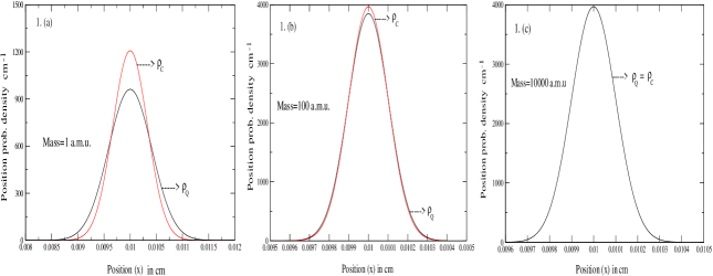
Figure 1: The position probability densities ${\rho}_{Q}(x,t)$ and ${\rho}_{C}(x,t)$ are plotted for varying mass of the particles (in atomic mass units) with ${\sigma_{0}}=10^{-5}$ cm, $u=10^{3}$ cm/sec, C=10 and t=$10^{-5}$ sec.

All the density functions are assumed to be normalized and $D(x,p,t)$ satisfies the classical Liouville’s equationssg given by

$$\frac{\partial D(x,p,t)}{\partial t}+{\dot{x}}\frac{\partial D(x,p,t)}{\partial x}+{\dot{p}}\frac{\partial D(x,p,t)}{\partial p}=0$$ (13)

Since for free particles ${\dot{p}}=0$ and ${\dot{x}}=p/m$ we have

$$\frac{\partial D(x,p,t)}{\partial t}+\frac{p}{m}\frac{\partial D(x,p,t)}{\partial x}=0$$ (14)

Integrating the above equation with respect to $p$ one gets

$$\frac{\partial{\rho_{C}}(x,t)}{\partial t}+\frac{\partial}{\partial x}\left[\frac{1}{m}{\bar{p}}(x,t){\rho_{C}}(x,t)\right]=0$$ (15)

where ${\bar{p}}={\int pD(x,p,t)dp}/{\int D(x,p,t)dp}$ is the ensemble average of the momentum. Defining ${\bar{v}}(x,t)={{\bar{p}}(x,t)}/m$ as the average velocity, one obtains

$$\frac{\partial{\rho_{C}}(x,t)}{\partial t}+\frac{\partial}{\partial x}{J_{C}}(x,t)=0$$ (16)

where ${J_{C}}(x,t)$ and ${\bar{v}}(x,t)$ represent the mean motion of the continuum matter at $(x,t)$. Eq(s).(16) is the equation of continuity for the continuous density function $\rho_{C}(x,t)$ of a statistical ensemble of particles. The expression for the classical probability current density is given by

$${J_{C}}(x,t)=\frac{1}{m}{\int pD(x,p,t)dp}$$ (17)

and is related to the mean velocity by ${J_{C}}(x,t)=\rho_{C}(x,t){\bar{v}}(x,t)$.

Now substituting the expression for the time evolved phase space distribution function $D(x,p,t)$ from Eq(s).(9) in Eq(s).(17) we get the expression for the current density or the arrival time distribution at a particular detector location x=X for this classical ensemble of free particles given by

$${J_{C}}(x,t)=\rho_{C}(x,t)~{}\left\{u+\frac{(x-ut)\hbar^{2}t}{\left[\hbar^{2}t^{2}+4m^{2}{\sigma_{0}}^{4}(1+C^{2})\right]}\right\}$$ (18)

If we impose here the minimum uncertainty condition ${\it viz.}$, $C=0$ then one can check from Eq(s).(6), (7), (12) and (18) that both ${\rho_{Q}}(x,t)$=${\rho_{C}}(x,t)$ and ${J_{Q}}(X,t)={J_{C}}(X,t)$ hold, i.e., the classical and quantum probability currents are similar. Thus, if we take the initial phase space distribution function for the classical ensemble of particles as a product of two Gaussian functions matching with the initial quantum position and momentum distributions then the classical arrival time distribution exactly matches with the quantum one provided the minimum uncertainty relation is satisfied. But in general the quantum and classical distribution functions are different when the minimum uncertainty condition is not satisfied ($C\neq 0$).

Though ${J_{Q}}(X,t)$ and ${J_{C}}(X,t)$ are in general not equal for $C\neq 0$, the large mass limits of both are the same. This is seen from Figures 1 and 2 where the probability distributions and the currents are plotted respectively for different masses. It is apparent that in the large mass limit quantum distributions reduce to the classical distributions. The mass dependendence in the arrival time distributions and also in the position probability densities (for both the quantum and classical case) arises from the spreading of the wave packet.

Figure 2: The probability current densities $J_{Q}(x,t)$ and $J_{C}(x,t)$ are plotted for varying mass of the particles (in atomic mass units) at a detector location X=10 cm with ${\sigma_{0}}=10^{-4}$ cm, $u=10^{3}$ cm/sec, C=100.

We now compute the mean arrival time $\bar{\bf\tau}$ by substituting the expressions for the quantum current in Eq(s).(2). [One should note that though the integral in the numerator of Eq(s).(2) formally diverges logarithmically, several techniques have been employed in the literature hahne ensuring rapid fall off for the probability distributions asymptotically, so that convergent results are obtained for the integrated arrival time. Here we have employed a simple strategy of taking a cut-off ($t=T$) in the upper limit of the time integral with $T=(X+3\sigma_{T})/u$ where $\sigma_{T}$ is the width of the wave packet at time $T$. In other words, our computations of the arrival time are valid up to the $3\sigma$ level of spread in the wave function.] It is instructive to examine the variation of mean arrival time with the different parameters of the wave packet. In Figure 3 we have plotted the variation of $\bar{\bf\tau}$ with mass at different detector locations, keeping the group velocity $u$ and initial width $\sigma_{0}$ fixed. One sees that the mean arrival time calulated by using the quantum cur Cnt $J_{Q}(X,t)$ as the arrival time distribution asymptotically approaches the classical result in the limit of large mass.

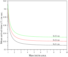
Figure 3: The mean arrival time $\bar{\bf\tau}$ is plotted against the mass of the particles (in atomic mass unit) at different detector locations $X=5.1$ cm, $X=5.2$ cm, and $X=5.3$ cm. for C=10, ${\sigma_{0}}=0.0001$ cm, $u=10$ cm/sec.

4.SUMMARY AND OUTLOOK

To summarize, in this paper we have investigated the quantum-to-classical transition of the mean arrival time defined through the probability current. We have formulated the classical arrival time distribution from the phase space distribution for a classical ensemble of particles. The expression for classical probability current constructed by us matches exactly with the quantum probability current in the limit of minimum uncertainty. We note that the uncertainty condition is not a stringent requirement for the case of the initial classical distribution. Thus the classical arrival time distribution $J_{C}(X,t)$ will in general be different from the quantum distribution $J_{Q}(X,t)$ if we do not impose the minimum uncertainty restriction on the initial distribution. This issue needs to be explored further in order to have a deeper understanding of the quantum-classical comparison of arrival time. However, in the present example that we have constructed, the quantum results for the probability current and through it the arrival time distribution, approaches the classical result in the large mass limit. A number of schemes others ; bohm ; finkelstein ; others1 have been suggested in the literature for calculating the arrival time distribution such as those based on axiomatic approaches, trajectory models of quantum mechanics, attempts to define and calculate the arrival time distribution using the consistent histories approach, and attempts of constructing the time of arrival operator, etc. It might be worthwhile to investigate the quantum-classical correspondence of the arrival time distribution using these different approaches. Such studies, if undertaken extensively, are not only expected to throw light on the comparitive merits of different arrival time formulations, but could also be of relevance to the behaviour of mesoscopic systems where a great deal of experimental activity is presently underway brandes .

Classically we know that a point particle with uniform motion will reach a particular location at a time which is independent of the mass of the particle and depends only on its uniform velocity. In the discussion of classical limit of quantum mechanics it is usually assumed that the peak mean position of the wave packet moves according to classical trajectory derived from the Ehrenfest theorem. It could be argued though that one should not expect to recover an individual classical trajectory when one takes the classical limit of quantum mechanics. Rather, one should expect the probability distributions of quantum mechanics to become equivalent to the probability distributions of an ensemble of classical trajectories. The current investigation is concerned about this particular approach to test the quantitative equivalence between the classical mechanical prediction and the prediction obtained in the macroscopic limit of quantum mechanics. Here, what we see is that the mean time of arrival of a freely moving quantum particle computed through the probability current depends on the mass of the particle even if its group velocity is fixed. So it turns out that the characteristic of mean time in this framework is different from that of mean position. The predicted mass dependence of mean arrival time is, in principle, amenable for experimental verification, and is a clear signature of the probability current approach to time in quantum mechanics leavens2 .

Acknowledgments

We would like to thank Late S. Sengupta, D. Home, C. R. Leavens and G. E. Hahne for useful discussions. AKP and MMA acknowledge the Senior Research Fellowships of the CSIR, India.

References

- (1) Einstein A in Scientific Papers Presented to Max Born (Oliver and Boyd, Edinberg, London, 1953 ) pp 33-40; Born M Kg. Dnsk. Vid. Selsk. Mat. Medd. 30 1 (1955); Born M and Ludwig W Z. Physik 150 106 (1958); de Broglie L Non-Linear Wave Mechanics, A Causal Interpretation (Elsevier, Amsterdam, 1960) p 136; Brown L S Am. J. Phys. 40 371 (1972); Home D and Sengupta S Am. J. Phys. 51 265(1983); Cabrera G G and Kiwi M Phys. Rev. A 36 2995(1987).
- (2) Einstein A in The Born-Einstein Letters (Macmillan, London, 1971) p 208.
- (3) Pauli W in The Born-Einstein Letters (Macmillan, London, 1971) p 221.
- (4) Home D Conceptual Foundations of Quantum Physics (Plenum Press, New York, 1997).
- (5) Lee H W Phys. Rep. 259 147-211 (1995), Hillery M, O’Conell R F, Scully M O, Wigner E P Phys. Rep. 106 121-167 (1984).
- (6) Muga J G and Leavens C R Phys. Rep. 338 353-438 (2000).
- (7) See for example, relevent recent reviews in Time in Quantum Mechanics, edited by Muga J G, Mayato R S and Egusquiza I L (Springer-Verlag, Berlin, 2002).
- (8) Muga J G, Brouard S, and Macias D Ann. Physics. (N.Y.) 240 351 (1995); Delgado V and Muga J G Phys. Rev. A 56 3425 (1997); Aharanov Y, Oppenheim J, Popescu S, Reznik B and Unruh W G Phys. Rev. A 57 4130 (1998); Halliwell J J and Zafiris E Phys. Rev. A 57 3351 (1998); Delgado V Phys. Rev. A 57 762 (1998); ibid 59 1010 (1999); Egusquiza I L and Muga J G Phys. Rev. A 62 032103 (2000); Oppenheim J, Reznik B and Unruh W J. Phys. A 35 7641 (2002); Damborenea J A, Egusquiza I L, Hegerfeldt G C and Muga J G Phys. Rev A 66 052104 (2002).
- (9) Dumont R S and Marchioro T L II Phys. Rev. A 47 85 (1993); Leavens C R Phys. Lett. A 178 27 (1993); Challinor A, Lasenby A, Somaroo S, Doran C and Gull S Phys. Lett. A 227 143 (1997); Leavens C R Phys. Lett. A 303 154 (2002); Muga J G, Brouard S and Macias D Ann. Phys. 240 351 (1995); Leavens C R in: Time in Quantum Mechanics edited by Muga J G, Mayato R S and Egusquiza I L (Springer-Verlag, Berlin, 2002) p 121.
- (10) Holland P Phys. Rev. A 60 4326 (1999); Holland P Ann. Phys. (Leipzig) 12 446 (2003); Holland P and Philippidis C Phys. Rev. A 67 062105 (2003).
- (11) Ali M M, Majumdar A S, Home D and Sengupta S Phys. Rev. A 68 042105 (2003).
- (12) Bohm D Phys. Rev. 85 166 (1952) ; Bohm D and Hiley B J The Undivided Universe (Routledge, London, 1993); Holland P The Quantum Theory of Motion (Cambridge University Press, London, 1993).
- (13) Leavens C R Phys. Lett. A 178 27 (1993); McKinnon W R and Leavens C R Phys. Rev. A 51 2748 (1995).
- (14) Bracken A J and Melloy G F J. Phys. A 27 2197 (1994).
- (15) Deotto E and Ghirardi G C Found. Phys. 28 1 (1998).
- (16) Finkelstein J Phys. Rev. A 59 3218 (1999).
- (17) Gurtler R and Hestenes D J. Math. Phys. 16 573 (1975); Hestenes D Am. J. Phys. 47 399 (1979).
- (18) Kemmer N Proc. Roy. Soc. Lond. A 173 91 (1939).
- (19) Struyve W, Baere W D, Neve J D and Weirdt S D Phys. Lett. A 322 84 (2004).
- (20) Ford G W and O’Connell R F Am. J. Phys. 70 319 (2002); Robinett R W, Doncheski M A and Bassett L C Preprint quant-ph/0502097 (2005).
- (21) Das S K and Sengupta S Current Science 83 1234 (2002).
- (22) Damborenea J A, Egusquiza I L, and Muga J G Preprint quant-ph/0109151 (2003); Hahne G E J. Phys. A 36 7149 (2003).
- (23) Aharonov Y and Bohm D Phys. Rev. 122 1649 (1961); Kijowski J Rept. Math. Phys. 6 361 (1974); Yamada N and Takagi S Prog. Theor. Phys. 86 599 (1991); Brouard S, Mayato R S and Muga J G Phys. Rev. A 49 4312 (1994); Busch P, Grabowski M and Lahti P J Phys. Lett. A 191 357 (1994); Grot N, Rovelli C and Tate R S Phys. Rev. A 54 4676 (1996); Delgado V and Muga J G Phys. Rev. A 56 3425 (1997); Galapon E A J. Math. Phys. 45 3180 (2004); Gambini R, Porto R A and Pullin J New J. Phys. 6 45 (2004); Ruseckas J and Kaulakys B Lith. J. Phys. 44 161 (2004).
- (24) For a recent review, see, Brandes T Phys. Rep. 408 315 (2005).